


Abstract
There has been substantial interest of late on the issue of coherence as a resource in quantum thermodynamics. To date, however, analyses have focused on somewhat artificial theoretical models. We seek to bring these ideas closer to experimental investigation by examining the 'catalytic' nature of quantum optical coherence. Here the interaction of a coherent state cavity field with a sequence of two-level atoms is considered, a state ubiquitous in quantum optics as a model of a stable, classical source of light. The Jaynes–Cummings interaction Hamiltonian is used, so that an exact solution for the dynamics can be formed, and the evolution of the atomic and cavity states with each atom-field interaction analysed. In this way, the degradation of the coherent state is examined as coherence is transferred to the sequence of atoms. The associated degradation of the coherence in the cavity mode is significant in the context of the use of coherence as a thermodynamic resource.
Export citation and abstract BibTeX RIS

Original content from this work may be used under the terms of the Creative Commons Attribution 4.0 licence. Any further distribution of this work must maintain attribution to the author(s) and the title of the work, journal citation and DOI.
1. Introduction
The study of coherence in optics, and later quantum optics, has a long history, from Young's famous experiments demonstrating the wave nature of light [1], to the development of the quantum optical description of coherence [2–5]. Indeed the description of coherence through correlation functions of the field is arguably the central concern of quantum optics, and has been fundamental to e.g. stellar intensity interferometry [6, 7], understanding the ultimate noise limits to interferometric measurements [8, 9], and providing experimental evidence for the particle nature of light [10].
In recent years there has been a resurgence of interest in coherence, in the nascent field of quantum thermodynamics [11–14]. Here, coherence is taken to mean specifically superposition in the energy eigenbasis (or more generally off-diagonal elements of the density matrix in this basis). Indeed, in the study of thermodynamics, there are two stark differences between the classical regime of textbook statistical mechanics and the quantum regime of small numbers of constituent particles. One is that in this limit, the size of fluctuations of thermodynamical quantities are comparable to their mean values, and a thermodynamical system is no longer well-characterized by mean properties [15–18]. The other is the existence of superpositions in the quantum theory [19]. Just as the understanding of classical thermodynamics gave rise to the steam engine and the industrial revolution, developing its quantum counterpart is crucial to harnessing the full power of quantum and nano devices to develop new quantum technologies. Central to this endeavour is exploring the role of coherence in quantum thermodynamics.
In the quantum information inspired resource theory approach, coherence is thought of as a resource [20–26], enabling (at least approximately) non-energy conserving operations which would otherwise be forbidden [27, 28]. Although coherence cannot be created under strictly energy conserving operations, under certain circumstances it may be shown that a coherent reservoir can enable a coherent operation on an external system with an accuracy that does not degrade upon use. This paradoxical result led to the suggestion that coherence could be used catalytically [29]. The resolution is provided by careful consideration of correlations between systems which have interacted with the reservoir [30], a point we return to later.
In this paper we examine the distribution of coherence amongst systems, in the sequential interaction of a single mode coherent state with a series of two level systems through the Jaynes–Cummings interaction. There are two good reasons for addressing the issue of coherence as a resource in this way: firstly the Jaynes–Cummings model is very well understood and there are long-established techniques for analysing it [31–34], and secondly it is possible to realise it experimentally using techniques from cavity quantum electrodynamics [35].
We consider a sequence of two-level atoms introduced, one at a time, into a cavity prepared in an initial coherent state. The atoms are prepared in their excited states and the cavity transit time is chosen so as to prepare the emerging atoms, at least approximately, in an equally-weighted superposition of the ground and excited states,  and
and  . A diagram of this setup is shown in figure 1. The phase of the superposition is determined by the phase of the coherent state of the cavity mode. Such interactions are of central importance in quantum information [36, 37] and also in quantum thermodynamics, as it is these which may be used to extract maximal work from coherence [29, 38, 39, 19, 40, 41]. We evaluate how the fidelity of the final state changes with subsequent interactions, and analyse the results in the light of [29].

Figure 1. Schematic of the interaction of the coherent state cavity field with a two-level atom. Each atom is initialized in the excited state, and leaves the cavity in a superposition state.
Download figure:
Standard image High-resolution imageA quantum optical coherent state is the canonical example of a source of coherence. This is because it forms the closest approximation to an ideal, perfectly stable, classical field with a well-determined amplitude and phase. Indeed a field in a coherent state is precisely equivalent to a superposition of such a classical field and the vacuum [42]. The quantum optical properties of coherent states have been well studied, and in the sense of enabling operations, discussed above, lasers are routinely used as control fields to induce quantum operations on the electronic states of trapped atoms and ions [43, 44]. Indeed it is in such systems that the highest achieved fidelities for coherent operations have been demonstrated, among all physical systems proposed for use in quantum information processing [45]. If the coherent state amplitude is high enough, the state is essentially classical, and the back action of the field due to the interaction may be neglected, a situation strongly reminiscent of the proposed catalytic use of a source of coherence. Yet if the amplitude is finite, then this back action cannot be disregarded: it is this which we explore in this paper.
Cavity quantum electrodynamics experiments have to contend with the inevitable effects of losses from the cavity due to the finite reflectivity of the mirrors [35]. These losses provide a further and unavoidable loss of coherence [46] that impacts the state of the cavity field and disrupts the Jaynes–Cummings dynamics [47]. In this paper we opt not to include cavity losses for the crucial reason that to do so would mask the effect we are seeking to explore, namely the quantitative consumption of coherence as the field is repeatedly employed. To include the cavity losses would add a further decohering mechanism, and would render it difficult to account for the loss of coherence purely associated with coherence as a finite resource.
We note that the Jaynes–Cummings Hamiltonian is considered as an example in [29], with the field state in an equal superposition over a fixed range of energy eigenstates, rather than using a coherent state of the field. For the parameters considered it was found that increasing the average energy without any increase of the number of terms in the superposition (a measure of the amount of coherence in such a state) improves performance when the field is used as a reservoir of coherence. For a coherent state there is no longer a clean separation of average energy and the spread of the superposition: both are determined by a single parameter, the average photon number. This complicates the analysis somewhat, but is of considerable physical relevance due to the ubiquity of experimental systems employing coherent state control fields in the Jaynes–Cummings interaction.
The paper is divided as follows. In section 2 we introduce the concept of coherence and its role in quantum thermodynamics. Section 3 provides a brief review of the Jaynes–Cummings model, and the coherent operations it performs on a sequence of two-level atoms in a coherent state field is investigated in section 4. Here, we present both analytical and numerical analyses of the evolution of the cavity field upon this sequential interaction. In section 5, these results are discussed alongside those of the scheme for catalytic coherence proposed in [29], before a summary of our results is given in the final section.
2. Coherence as a resource
Let us start with a brief overview of the concept of coherence and its relevance as a (thermodynamic) resource. The key idea is that as coherence can be used as a thermodynamic resource it must be consumed as it is used. Were this not the case then one might envisage coherent free-energy, and perpetual motion machines or other absurdities. In the following, by coherence we mean specifically the property of a state being in a quantum superposition of different energy eigenstates, as opposed to a single eigenstate, or a statistical mixture. A good measure of how much coherence a state exhibits is, for example, the off-diagonal entries of its density matrix in the energy eigenbasis (see for example [22, 24] for further definitions of coherence measures). A 'classical' mixed state would only have entries on the diagonal, so it is useful to think of coherence as non-classicality of a state.
The field of thermodynamics traditionally only deals with statistical mixtures of energy eigenstates, so that taking coherence into the picture fundamentally changes some of its basic principles, indeed it may fairly be stated that the inclusion of superposition is the principal defining feature of quantum thermodynamics [11, 12]. In particular, it can be shown that more work can be extracted from a system that exhibits coherence than from an incoherent system (a system without any coherence) with exactly the same energy probability distribution. Let us illustrate this with a simple example. Suppose we have two identical baths of two-level atoms at equal temperature, as shown in figure 2(a). One atom from each bath is chosen randomly and interacts with the other via the interaction

as illustrated in figure 2(b). Here,  and
and  are the atomic raising and lowering operators, respectively, so that the interaction mediates an energy exchange between the atoms. If the atoms are in a statistical mixture, as described by the thermal density matrix

then no energy will flow on average, as predicted by classical thermodynamics. If the atoms are returned to their reservoirs and the process is repeated then there will be no net energy exchanged between the reservoirs.

Figure 2. Possible energy transfer protocol between two identical reservoirs using coherence. (a) The initial state, with both baths having the same energy distributions. (b) One atom from each bath is chosen randomly, and allowed to interact via (1). (c) If the atoms are initially in coherent superpositions, then an interaction time can be chosen such that the atom from the right reservoir ends up with more energy than the left, so that the average energy in the right reservoir increases while it decreases on the left. Such heat difference could then be used to drive a heat pump, for example. If the atoms are instead described by a statistical mixture, no energy transfer between the reservoirs is possible: quantum coherence enables the work extraction.
Download figure:
Standard image High-resolution imageNow let us consider what happens if the atoms are instead described by coherent superposition states. We replace the thermal mixture (2) with the coherent quantum state

for each atom (in both baths). This system has the same energy probability distribution as the classical thermal states. However, under time evolution of the interaction Hamiltonian  , the two atoms in contact now perform coherent oscillations, so that the joint state of these atoms after time t is given by

Knowing the phase of the initial atoms, we can choose an interaction time  to maximize the amplitude of
  compared to the the state
  , producing the two-atom state

Thus the second atom ends up with more energy than the other. When the atoms are returned to their respective reservoirs, the right reservoir gains energy on average (figure 2(c)). As this process is repeated, energy is steadily extracted from the first reservoir and deposited in the second. Such a setup could then be used, for example, to drive a heat pump, and in this way, work extracted from the system. This simple example illustrates that the presence of coherence enables operations that would otherwise be thermodynamically forbidden, so that coherence can be exploited as a source of work. In a sense, this is not surprising, as coherence is just another form of knowledge about the system which we can use to extract energy: although the coherent bath has the same energy probability distribution as the incoherent one, it has zero entropy.
Coherence fundamentally changes how we have to think about thermodynamics. Its function as a thermodynamic resource from which one can extract work [19, 25, 40, 39], means it is of great importance to study how coherence can be distributed amongst systems, or generated under given constraints. These questions of creating and transforming coherence are examined in the resource theory of coherence1 . It can be shown that coherence does not increase under strictly energy preserving operations, that is, operations that commute with the system Hamiltonian. However, by allowing correlations to build up, it is possible to put an arbitrary number of systems into approximate coherent superpositions with the help of an infinite-dimensional reference system acting as a catalyst [29, 30, 48]2 . In this work, we are interested in a variation of this coherence 'catalysis' in which an optical coherent state acts as our reference system. We examine a realistic scheme of redistributing coherence from a coherent state reservoir to a sequence of two-level atoms, and study how this resource becomes degraded upon use. This is pertinent in consideration of the possible extraction of work from coherence, as discussed above.
3. Jaynes–Cummings model
The Jaynes–Cummings model [31–34] describes the interaction of a two-level system, such as two levels of an atom, resonantly coupled with a bosonic mode, for example the electromagnetic field inside a cavity, in the rotating wave approximation. The interaction Hamiltonian is given by

where  and
and  are the usual bosonic ladder operators and
  the atomic lowering and raising operators. In the rotating wave approximation the total number of excitations is a constant of the motion, and the effect of the interaction is to induce a unitary operation within subspaces of constant total energy, giving an exactly solvable model for atom-light interaction.
3.1. Semiclassical behaviour
Before investigating the Jaynes–Cummings evolution, it is worthwhile to pause and consider the simpler, semiclassical Rabi problem in which the quantized field mode is replaced by a classical field [5, 34]. In this model, the single-mode creation and annihilation operators are replaced by a c-number amplitude so that our model Hamiltonian becomes

We can write the atomic state in this interaction picture as a superposition of the excited and ground states in the form

where direct solution of the Schrödinger equation, for an atom prepared in its excited state gives

Note that the phase of the field amplitude, α, has been imprinted onto the phase of the atomic superposition state. If we choose the interaction time such that  then the atom is left in the equally weighted superposition state
  . There is no back-action on the field here, as it has been treated classically. In principle this process can be repeated at will with each new atom being transformed into this same superposition state. To treat the coherence as a resource, however, we need to quantize the field mode and keep track of the effects of the interaction both on the atoms and also on the state of the field.
3.2. Fully quantum behaviour
The fully quantum Jaynes–Cummings Hamiltonian (6) conserves the total number of quanta and this feature makes it possible to find an exact solution for the dynamics. In general a pure state of the atom and field mode will be of the form

Evolution under the Schrödinger equation with Hamiltonian (6) gives a set of coupled, linear differential equations which are readily solved to give the exact dynamics at any given time:

The evolution of an initially excited atom interacting with an arbitrary cavity state,  , is thus given by

This may be understood as the initial excitation of the atom oscillating between the cavity and the atom. Note that the frequency of this oscillation is different in each constant energy subspace, and depends on the total excitation number n + 1: thus as time progresses the oscillations for different total energy drift in and out of phase, giving rise to the famous collapses and revivals of the Jaynes–Cummings model [32–35]. Our interest, however, is in interaction times that are much shorter than the collapse and revival times.
A key feature of the evolution is that at any given time (after the initial time) the atom and field mode will be in an entangled state and it is this entanglement that encapsulates the back action on the state of the field mode. As discussed, we are concerned with a field mode prepared in an initial coherent state interacting with a sequence of atoms, shown schematically in figure 1, each prepared in its excited state, a situation that is reminiscent of the Scully–Lamb theory of the laser [49]. Here, however, we are interested in the combined atom field state that is prepared and the associated effects on the coherence.
4. Coherent operations in the Jaynes–Cummings model
Armed with the exact atom-field state in equation (12), we are now ready to analyse the performance when a cavity coherent state is used as a resource to induce coherent operations on a succession of atoms. By inspection of (12) it is clear that after a quarter of the first Rabi period the atom will be found in the coherent superposition state  with high probability, provided three conditions are met. The first, and simplest, is that we choose the initial cavity state such that the phase θ is imprinted on the atomic state. We can achieve this by choosing a state for which
  . The second is that the spread in Rabi frequencies is small compared to the central frequency, or in other words, the spread in photon number is small compared to the mean photon number, so that it is possible to choose t1 satisfying
  for all n with appreciable amplitude in the superposition. The final condition is that the distribution cn is such that the shifted state, with one additional photon in the field, has large overlap with the initial state. There is a tension or complementarity between these two conditions: a narrower distribution means the former condition is readily satisfied, but requires a sharper change in the coefficients cn, making the second more difficult to meet. This is a feature of the form of the Jaynes–Cummings interaction, and for a flat distribution over a given range (
 ) means that simply increasing the average energy improves performance, as noted in [29].
We are interested in particular in the case in which the field is in a coherent state  . The phase we wish to imprint onto the atom, θ, is then simply the argument of the complex amplitude α. For convenience and without loss of generality we take α to be real and positive corresponding to θ = 0, aiming at the creation of a target superposition state
  . Substituting into (12), rewriting in the
  basis and shifting the second term in the sum gives

We wish to maximize the fidelity of the output state with  (maximize the probability of obtaining
  ), or equivalently minimize the fidelity with the state
  (the probability of finding the atom in
  ). After an interaction time t1 this latter probability is:
where  and
and  . Each term in the sum is positive, and for large
  ,
,  for all n with non-negligible amplitude. Thus we should choose
  . We choose an interaction time t1 defined by

giving

which tends to zero in the limit of large  . This was to be expected, as in the limit of large
  the coherent cavity state behaves like a classical field, and the desired coherent operation may be achieved perfectly. A detailed analytical derivation of this approximation including second order terms can be found in appendix A 3
.
the coherent cavity state behaves like a classical field, and the desired coherent operation may be achieved perfectly. A detailed analytical derivation of this approximation including second order terms can be found in appendix A 3
.
4.1. Effect of the interaction on the field
Another important effect of large but finite  concerns the back-action of the interaction on the field: how is the resource, that is the state of the cavity mode, degraded upon use? Had we chosen to use atoms prepared in the ground state, then the coherence would inevitably be consumed as the light was gradually removed from the cavity by the sequence of atoms. By starting with atoms in excited states, however, this elementary coherence-removing process is avoided and we are left only with the consequences of the fundamental degradation of the quantum coherence.
After a single atom has passed through the cavity, the joint state of cavity and atom is given by equation (13), where for convenience we return to the  ,
,  basis of the atom:

We consider again the large  limit, and for an interaction time t1 satisfying equation (15), it may be shown that the approximate atom-field state after interaction is given by:

where

The approximations leading to this result are straightforward but lengthy, and the full technical details are given in appendix B. The change in the field thus has a clear physical interpretation: an initial coherent state  is transformed to a mixture of coherent states, one shifted down in amplitude with probability 1/2 to a state with average photon number α2 − π/4, and the other shifted up in amplitude with probability 1/2 to a state with average photon number α2 + 1 + π/4. It follows that the average photon number in the cavity field is increased by (approximately) 1/2, as half an excitation is transferred from the atom to the field:

When the process is repeated upon introduction of a second atom to the field, the interaction time is now chosen such that the probability of success is maximal for a coherent state with this increased average photon number,  . The probability of failure, that is of finding the atom in the
  state, is the average of the probability of failure for each of the two shifted coherent states
  and
and  . Remarkably, this second round of atom-field interaction results in a slight increase in fidelity with the desired
  state in the next round, at order
  , due to the increased average photon number. Numerical results for α = 10, corresponding to a mean photon number of
  , are shown in table 1.
Table 1. Probabilities after two atom-field interactions for α = 10 with adjustment of interaction times after the first cycle. Bold digits show the deviation from the corresponding single-atom probabilities for easier comparison.
| P(+1) | P(+2) |

|
P(+2)P(+1) |

|
|---|---|---|---|---|
| 0.995909 | 0.995915 | 0.995932 | 0.991841 | 0.991858 |
| P(−1) | P(−2) |

|
P(+2)P(−1) |

|
| 0.004091 | 0.004085 | 0.991631 | 0.004074 | 0.004056 |
The ability of the coherent state cavity field for inducing coherent operations under the Jaynes–Cummings interaction is therefore not degraded upon first use: remarkably, it is slightly improved. It is worthwhile pointing out that although this result may be surprising, it is not unphysical. We should expect, however, that a fixed initial amount of coherence may not be used to produce independent copies of the equal superposition state  indefinitely. A complete picture requires us to consider both the many copy limit, and correlations between subsequent atoms from each interaction.
4.2. Evolution of the cavity state with subsequent interactions
We now wish to derive the evolution of the field under successive interactions with subsequent atoms. We recall that following the first interaction, the cavity state is a mixture of two different coherent states with slightly different amplitudes, as shown in equation (18), and for the second atom we choose an interaction time satisfying  , where
  . However, for each coherent state
  ,
,  in the mixture, there is now a slight mis-match between the amplitude squared
  (
( ) and
) and  , used to define the interaction time. If this mis-match is too large, the chosen interaction time will not produce the desired evolution. We begin by considering the consequences of this mis-match on the effect of the interaction on the cavity state in subsequent rounds.
Let us consider an element of the mixture  , with

where  is the average photon number of the field after r interactions, and δ is a real number, introduced to quantify the mis-match between
  and
and  . After a single interaction,
  and
and  . However, we assume in the following only that δ is small compared with α2 in order that the analysis can be applied to subsequent rounds. We wish to show that under successive interactions the state of the field remains a mixture of coherent states, parametrized by δ, and to derive the change in δ over time. In this regime, it can be shown (see appendix C) that for an element
  of the mixture, after r interactions, the approximate state after one further interaction is indeed given by:

where


The change in the field thus retains the physical interpretation given for the first round, as analysed in 4.1, but with modified probabilities. An initial coherent state  is transformed to a mixture of coherent states: one is again shifted down in amplitude to a state with average photon number α'2−π/4, but now with probability
  , while the other is shifted up in amplitude to a state with average photon number α2 + 1 + π/4, but with a modified probability of
  . At the end of each round
  for the field as a whole (taking into account all components
  of the mixture) increases by 1/2, and δ shifts by
  .
.
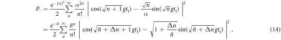
Recall that we have been assuming throughout that δ is small compared with α2. We finally note that if δ becomes comparable to α2, the scheme breaks down. Indeed equation (14) becomes:

where  . If δ ∼ O(α'2) then Δn is the same order of magnitude as
  , and it no longer holds that
  . As a result this probability of failure no longer scales as
  , and the scheme breaks down.
We now have enough information to understand the evolution of the state of the field under sequential interactions with multiple atoms. At the start of the process, the field is in a coherent state  , with
  , and δ = 0. After a single interaction, derived in detail in the previous subsection and in appendix B, the field is an equal mixture of two coherent states
  ,
,  ,
,  , and
, and  . Here, δ ≪ α and thus in each subsequent round δ shifts up or down with (approximately) equal probability, in steps of
  . In other words, δ performs a classical, unbiased random walk with step size
  . After r steps, with r ≪ α, the expectation value of δ is zero, with a spread of
  [50].
[50].
After r ≃ α2 steps, the spread of the distribution, and typical values of δ, are therefore  . At this stage the probabilities of shifting up or down in δ have become slightly asymmetric, as described in the analysis above. For δ > 0, the probability of an increase in δ is slightly bigger than the probability of a decrease. The converse is true for δ < 0. A possible evolution of δ with the number of steps r is shown in figure 3 to illustrate this result. Thus those elements of the mixture
  with higher amplitude-squared than the mean photon number tend to shift up further in number, while those with lower amplitude-squared tend to shift down further, leading to a faster spread in the distribution. Let us consider a coherent state
  with amplitude near the upper end of the distribution, with δu positive and
  , where the subscript u indicates we are considering the upper end of the distribution. At the next interaction,

Figure 3. A possible evolution of the mis-match  with the number of steps r. When r ≪ α2, δ performs a classical random walk, but for r ≃ α2, the probabilities of shifting up or down in δ become asymmetric, leading to an overall increase in δ for δ > 0.
Download figure:
Standard image High-resolution imageThus the random walk is now biased and the expectation value for  increases slightly:

In subsequent rounds, this expectation value increases each time by a multiplicative factor, so that after a further k interactions, we find

Recalling that the exponential function may be defined by the limit  of
of  , and noting that we are considering α2 ≫ 1, it is convenient to express the number of rounds k as a multiple of α2, k = l α2. In this case we find4

Thus for  and an initial
  , then
  , and the protocol begins to fail for subsequent interactions. We can make a similar argument for δl < 0, for those elements
  with amplitudes at the lower end of the distribution. Thus we find that after at most
  interactions, the state of the field is no longer useful for enabling coherent operations through the Jaynes–Cummings interaction.
As described above, for  interactions however, the approximations derived for the single interaction case still hold, and we can expect that the atom-field interactions produce
  approximate copies of
  from the initial stream of atoms, each prepared in its excited state
  .
.
4.3. Correlations between atoms
The ability of the cavity state to approximately induce the desired operation is, however, only part of the picture. Correlations build up between the atom and the field as a result of the interaction, and between subsequent atoms via the field. As shown previously [30], neglecting such correlations can lead us to conclude paradoxical and unphysical effects. In the remainder of this section, we explore the correlations that build up between subsequent atoms in the Jaynes–Cummings interaction.
Conditional probabilities after two rounds, given in table 1 for α = 10, illustrate these correlations between successive atoms. We see that the probabilities after the second atom-field interaction depend strongly on the outcome of the first round: the probability of failure given that the first atom ended up in the state  is more than twice as large as if the first atom ended up in the state
  .
.
To further understand the correlations, we begin by studying the state of the cavity conditioned on the state of the first atom. Conditional on the atom being found in state  or
or  , the cavity is projected to the state

a superposition of coherent states with slightly different average photon number, the phase of which is determined by the observed superposition state of the atom.
Recall that the performance of the scheme for an arbitrary cavity state depends both on the width of the photon number distribution (a narrow distribution implies a unique optimal interaction time) and the overlap of the initial state with a shifted state (one that contains an additional photon in the field). Figure 4 shows the photon number distribution of the cavity field conditional on atomic state  or
or  after the first round. Both resultant states have large overlap with the same states shifted up in average photon number, so that they may both be used as a coherence resource for subsequent interactions; a failed interaction does not destroy the reservoir coherence, as found in similar scenarios [30]. Note, however, that the cavity state conditioned on failure for the first atom has a wider distribution in photon number than in the case of success. Moreover, the distribution
  has two peaks, suggesting that there is no unique optimal interaction time for the next round. Let us return to equation (28): for the positive phase superposition there is constructive interference for photon numbers near the centre of the distribution P(n), while for the negative superposition this interference is destructive, and only the wings of the distribution remain, as reflected in figure 4. This leads to a larger spread in Rabi frequencies, so that the chosen interaction time is not a good approximation to a quarter-cycle in each constant excitation number subspace: the observed decrease in probability of success seen in table 1 is a result of this effect.

Figure 4. Normalized photon number distribution of the cavity field after one successful (blue) or failed (orange) interaction for an initial coherent state of α = 10.
Download figure:
Standard image High-resolution imageAgain considering the positive phase superposition in equation (28), we observe that the relative photon number variance  is decreased when the first atom is successfully produced in the state
  : for our numerical example of α = 10, the variance of the photon number distribution
  is given by5

An analysis of the success probabilities for squeezed cavity states shows that reducing the variance of the number distribution can lead to higher success probabilities up to a certain squeezing strength (see appendix D for details). Considering the effect of distribution width alone (rather than state overlap), the results suggest that after successful interactions the performance of the coherent state cavity field will be enhanced as the distribution narrows, but that this effect only works up to a certain point: when the variance of the cavity state reaches  , the success probability will peak and can only decrease upon further squeezing.
So far we have considered just two rounds; upon interaction with a sequence of atoms, the cavity field becomes correlated with each subsequent atom, thus also inducing correlations between atoms. Figure 5 shows the conditional success probabilities for preparing the atom in the state  for the rth atom after r − 1 successful or unsuccessful attempts with the preceding r − 1 atoms. In the case of success for each atom, as shown in the left-hand plot, an increase of the success probability with the number of atoms is beyond what can be expected due to the increase of the mean photon number in the cavity alone. This supports the idea that the deformation, or squeezing [5, 34], of the cavity state indeed acts to enhance the probability of success.

Figure 5. Left: probability for the last (rth) qubit to be found in the  state after all previous were measured in
  . The dashed line shows the probability for obtaining the state
  when the cavity field starts in a new coherent state with an increased photon number of 1/2 per each step. Right: probability for the rth qubit to end up in the state
  after all previous were measured in
  . In both cases the initial state α = 10 was used.
Download figure:
Standard image High-resolution imageTo confirm the squeezing of the number variance with each round, the evolution of the number and phase uncertainty during the first three interactions are shown in figure 6. The phase probability distribution, given by [5, 51–53, 34]

shows an increase in variance with each atom: this complements the decrease of the number variance, so that the total uncertainty of the state remains unchanged. Note that when considering the mixed cavity state unconditional upon previous outcomes, both the phase and number variances increase and the total uncertainty  increases by around 2% in our example.

Figure 6. Evolution of the number (orange) and phase (blue) uncertainties of the cavity state—initially with α = 10—after several interactions. The lines show the variance of exact coherent states when assuming an increase of half a photon per cycle, filled circles show the variance of the cavity state after all atoms have been found in  , empty circles show the variance of the mixed cavity state without any information on the atomic states.
Download figure:
Standard image High-resolution imageThe second graph in figure 5 shows that after initial failure, the success probability for the next interaction is only slightly reduced; an effect which does not change significantly when more unsuccessful outcomes occur. To observe how the probability of successive failure scales with α (or  ) in the Jaynes–Cummings model, a plot of the numerically calculated failure probability as a function of α is shown in figure 7, for the first five interactions which leave the atoms in the state
  . Alongside these plots are shown trend lines, which allow us to estimate the dependence of
  on
on  as
as

Recalling that the probability of failure in the first round is  , this
  dependence indicates that probabilities of multiple failures scales like the product of single-round probabilities, such that subsequent atoms are only weakly correlated.

Figure 7. Double-logarithmic plot of the probability for all atoms to end up in the state  during one to five rounds as a function of α. The graphs were obtained from numerical calculations with the interaction times updated to suit the increased cavity photon number with each interaction. The dotted lines show power series 0.3667α−1.954, 0.2693α−3.899, 0.3064α−5.847, 0.4884α−7.805 and 1.0225α−9.772 (top to bottom) obtained from fitting the numerical data for α > 3.
Download figure:
Standard image High-resolution imageFinally, to aid in visualizing the evolution of the cavity state upon successive interactions, figures 8–11 (video online is available at stacks.iop.org/NJP/22/043008/mmedia) show the Husimi Q-function

in phase-space [34] for the first 9 interactions. Figures 8–10 show the distribution for successful and unsuccessful interactions (i.e. conditioned on  ,
,  respectively), while figure 11 shows the state of the mixed (reduced) density matrix of the cavity when ignoring any information about the atomic states. Each successful interaction (figure 8) moves the centre of the distribution to higher q and therefore higher photon number, while deforming it such that the spread in this direction is squeezed to lower photon number variance. As can be seen in figure 9, failure to produce the state
  leads to a complete change in the shape of the distribution, with a dip appearing at the centre after one interaction. This is a feature of the fact that the cavity is projected into a negative superposition of two similar states when the first atom is found in the state
  . Repeated failure increases the size of this hole until the outer wing of the distribution is eliminated, and the state is pushed further towards a (squeezed) vacuum state. Interestingly, even after finding an atom in the state
  once, subsequent successful interactions can still somewhat compensate for the initial breakdown, as they bring the cavity closer to a coherent state with higher photon number again. This behaviour can be seen in figure 10: a successful outcome at any stage in the sequence of success and failure acts to squeeze the distribution and move it towards higher q.
Figure 8. Phase-space representation of the cavity state before and after 3, 6 and 9 successive interactions, conditioned on finding all involved atoms in the state  .
.
Download figure:
Standard image High-resolution image
Figure 9. Phase-space representation of the cavity state before and after 3, 6 and 9 successive interactions, conditioned on finding all involved atoms in the state  .
.
Download figure:
Standard image High-resolution image
Figure 10. Phase-space representation of the cavity state after 1, 3, 6 and 9 successive interactions, conditioned on finding the first atom in the state  and all subsequent atoms in the state
  .
.
Download figure:
Standard image High-resolution image
Figure 11. Phase-space representation of the mixed cavity state (unconditioned of the atomic states) before and after 3, 6 and 9 successive interactions.
Download figure:
Standard image High-resolution image5. Coherence catalysis
Our analysis in the previous sections shows that use of a quantum optical coherent state to induce coherent operations on a sequence of atoms under the Jaynes–Cummings interaction does not initially degrade the resource; we have seen that there is indeed an initial improvement in performance. The cavity field may be used  times before the coherence begins to degrade, after which performance degrades sufficiently quickly that the protocol no longer works. We have further found that subsequent atoms are only weakly correlated, and to a good approximation, the procedure produces independent copies of the desired superposition state
  . In this final section we review briefly the scheme for catalytic coherence proposed by Åberg [29], and compare the features of this scheme to our own.
The specific resource considered in [29] is an infinite-dimensional quantum system in a coherent superposition of energy eigenstates, given by

which we denote a 'ladder' state. For simplicity and without loss of generality we consider the relative phase θ = 0. The desired operation on the atom

can be approximately realized by an interaction of the form

where the first part acts on the Hilbert space of the atom and the operator  acts to shift the reservoir up or down in energy according to which atomic state has been produced. This interaction leaves the joint atom-reservoir system in the state

If the original state  , and the shifted state
  have a large overlap, then the state of the atom is close to the desired state. The reduced density matrix of the atom in the
  basis is given by

which is close to  for large L, the number of energy levels in the superposition state. The reservoir is left in a mixture of the initial state and another ladder state with a shifted offset,

Although not the same as the initial state, both parts of this mixture work equally well for a subsequent interaction, leading to the suggestion that the coherence can be used catalytically [29]. The analogy in the coherent state Jaynes–Cummings model that we have analysed here is that after a single interaction the cavity is left in a mixture of the states  ,
,  , with equal probabilities, where
  and
and  are given in equation (19). The former has slightly worse performance than the initial cavity state; the latter has slightly improved performance, and the mixture performs better overall. Thus, the ability of the reservoir to enable coherent operations is not left unchanged, as in the Åberg model, but is actually improved. One might be tempted to say that using the resource has, paradoxically, not used up the resource at all, but has added to it! This of course is not the case, and just as in the Åberg scheme, the resolution lies in careful consideration of the effect of repeated use, as we have shown.
5.1. Comparison of performance
Returning now to the Åberg scheme; the reservoir-induced operation works identically on each atom, so that the copies produced after each interaction are identical. They are not, however, independent: through the interaction with the reservoir, all of the atoms become correlated, and correlated too with the reservoir itself. Conditional on just one atom being found in state  , the reservoir collapses into the two-level state

such that the coherence of the reservoir is almost completely destroyed. Here,  is the probability for this to happen, which is very small for ladder states of large L, but crucially never zero. This is reflected in the success probabilities of multiple interactions, where it is seen that the probability of multiple failures does not decrease exponentially in the number of systems, but remains proportional to L−1 [30].
By contrast, in the Jaynes–Cummings scheme, the states of subsequent atoms are not identical, however they are (approximately) independent of each other. We have seen that over successive uses the many-copy probability of failure decreases exponentially, scaling like the product of individual failures. Only after  uses does the protocol begin to fail and performance rapidly declines for subsequent uses. Part of the story of the difference between the two schemes is thus the effect of failure on the reservoir of coherence.
In both schemes, after an atom interacts with the cavity the composite state is of the form

where  and
and  are the states of the field that couple with the atomic ground and excited states. After a single use, for the Åberg model these are
  and
and  , while for the Jaynes–Cummings model these are
  and
and  for subsequent uses the general expression has the same form. From equation (40), the density matrix of the atom after an interaction is straightforwardly given by

It follows that the probability of the atom being found in the state  after an interaction largely depends upon the inner product
  : if
: if ![$\mathrm{Re}\left[\langle {F}_{{\rm{e}}}| {F}_{{\rm{g}}}\rangle \right]\gt 0$](https://content.cld.iop.org/journals/1367-2630/22/4/043008/revision2/njpab7607ieqn162.gif) , then this probability is greater than 1/2. The closer it gets to zero, the more the atom is entangled with the cavity, and therefore its individual state is less well defined. Once it reaches
, then this probability is greater than 1/2. The closer it gets to zero, the more the atom is entangled with the cavity, and therefore its individual state is less well defined. Once it reaches ![$\mathrm{Re}\left[\langle {F}_{{\rm{e}}}| {F}_{{\rm{g}}}\rangle \right]\lt 0$](https://content.cld.iop.org/journals/1367-2630/22/4/043008/revision2/njpab7607ieqn163.gif) , the state
, the state  is more likely to be obtained, where now a larger negative value increases the probability of this outcome. The overlap between the state
  and
and  for the Jaynes–Cummings and Åberg models are shown in figure 12. The coefficient distributions, Cn of the state vectors in the energy basis
  for the Jaynes–Cummings model are given in the first column of the figure, while those for the Åberg model are displayed in the graphs in the second column. The first row represents
  and
and  in the first interaction. In each case there is a large overlap between these two distributions, leading to a high probability of success for the protocol. The second row shows
  and
and  after a failure in the first round: there is still a large area overlap between these two states in the Jaynes–Cummings case, while in the Åberg scheme the graphs do not overlap at all, and the qubit is found in either state
  or
or  with equal probability. Finally, the coefficient distributions upon two consecutive failures in the first two interactions are given in the third row. For the Åberg scheme, the overlap of the states
  and
and  is a negative number, corresponding to a higher probability of obtaining the state
  for the third atom following two failures. By contrast, even in the case of multiple consecutive failures, areas of overlap for the Jaynes–Cummings model are nonzero, but decreasing: the coherent state field may yet be used as a coherent resource, but with slightly decreased efficiency.
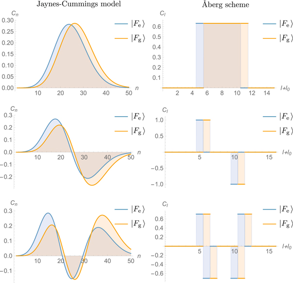
Figure 12. Comparison of the distributions of the coefficients of  and
and  between two schemes. The results for the coherent state cavity field in the Jaynes–Cummings model are shown on the left-hand column for a coherent state with α = 5, while those on the right show those of the Åberg scheme using a ladder state where L = 5. The coefficients of the state
  and
and  are denoted by the solid orange and blue lines respectively. The first row shows the distributions of the coefficients after the first atom-field interaction. The second row is the distributions following measurement of the atom after the first interaction in the undesired state. Analogously, the third row indicates the results supposing that
  is again obtained after the second interaction.
Download figure:
Standard image High-resolution imageThe effect on the cavity state is mirrored in the correlations introduced between subsequent systems, discussed previously. Analytical expressions for the joint probabilities for two consecutive interactions are given in table 2 for the Jaynes–Cummings interaction and the Åberg scheme [29, 30], in terms of  and L respectively. The state of the two atomic qubits after the interaction is non-separable in each case, since the joint probabilities show correlations. However, for the Jaynes–Cummings interaction these enter at second order only, such that the probabilities are independent to second order. The single-atom probabilities scale linearly
  in the Jaynes–Cummings case and 1/L in the Åberg scheme. However, the joint probabilities demonstrate the greater robustness of the Jaynes–Cummings model using coherent states against multiple failures: the probability for ending up in the state
  for two consecutive atoms in this case scales as
  compared to 1/L in Åberg's scheme. This is in agreement with the numerical results of figure 5.
Table 2.
Comparison of probabilities and joint probabilities obtained to  using coherent states in the Jaynes–Cummings interaction, and ladder states in the scheme proposed by Åberg [29]. The interaction time has been set such that
  , where μ is an arbitrary real number and
  .
.
| Coherent states in the Jaynes–Cummings model | Åberg scheme | |
|---|---|---|
| P(+) |

|

|
| P(−) |

|

|
| P(+) × P(+) |

|

|
| P(+) × P(−) |

|

|
| P(−) × P(+) |

|

|
| P(−) × P(−) |

|

|

|

|

|

|

|

|

|

|

|

|
|

|
We conclude with a plausability argument for how many copies one might reasonably expect to be able to extract from a reservoir of coherence. Consider r copies of the equal superposition state  :
:

where  denotes the permutation invariant, symmetric r-qubit state containing k zeroes and r − k ones. Note that each term in the superposition corresponds to a different total energy. The binomial distribution has mean k = r/2 and variation r/4. Thus the width of the distribution, the standard deviation, is
  . For large r, the distribution in this range is approximately flat with a steep fall off to zero outside [54], and we find an approximately equal superposition of energy eigenstates containing
  terms, corresponding to those values of k within
  of r/2.
For the ladder state  in the Åberg scheme, the reservoir state contains exactly L energy eigenstates in equal superposition. Thus, in terms of the coherence properties in the energy basis, r copies of
  is approximately equivalent to a ladder state of size
  . In other words, the ladder state
  is aproximately equivalent to L2 copies of
  . The scheme as given in [29] may be used to produce an indefinite number of identical mixed-state copies. However, as pointed out above, these are not independent, but rather are in a highly correlated joint state, with the initial coherence of the reservoir distributed across the joint state.
For the quantum optical coherent state the coefficients in the energy eigenbasis  are Poisson distributed with a mean and variance both equal to
  . Again in the limit of large
  this corresponds to an approximately equal superposition of
  terms, where each term in the superposition has a different total energy. Thus, in terms of the coherence properties in the energy basis, r copies of
  is approximately equivalent to a coherent state with average photon number
  . Thus we expect a coherent state
  to be able to create
  independent copies of
  before the protocol starts to break down. The Jaynes–Cummings interaction thus seems to be close to optimal for extracting coherence.
As a final note, if we therefore identify the 'size' of the state in the coherent state case as  and in the Åberg case as L, then we see that the error in the Jaynes–Cummings model scales as the inverse square of the size of the state,
  , while in the Åberg state the error scales as the inverse of the size of the resource 1/L. Thus for equivalent resources, the Jaynes–Cummings model produces better copies which are less correlated, and moreover repeated use improves the quality of the copies, for a moderate number of uses.
6. Conclusion
The study of coherence, a central concern of quantum optics for several decades, has taken on a new meaning in recent years with the advent of quantum thermodynamics. In particular it is now well-established that coherence can be used as a thermodynamic resource, one that allows tasks to be performed that are strictly prohibited in the absence of coherence. Our study has explored the nature of coherence as a resource whithin the coherent state Jaynes–Cummings model, familiar from quantum optics [31–35]. We explored the extent to which a sequence of two-level atoms, prepared initially in their excited state, could be prepared in a state close to a desired coherent superposition by interaction with a single cavity mode prepared, initially, in a coherent state.
Our main results are: the fidelity with which initially excited atomic states may be transformed to the equal superposition state  with the help of a quantum optical coherent state with average photon number
  scales as
  , and actually improves (at order
  ) with subsequent uses, at least initially. The probability of finding r atoms in the orthogonal state
  scales as
  , indicating that subsequent copies are almost independent after interaction with the cavity. The effect of successive interactions on the cavity state may be understood as causing the coherent state amplitude to undergo a classical random walk, and we showed that it is possible to create
  approximate copies of
  before the effectiveness of the cavity state as a resource begins to degrade. We find a weak correlation between subsequent copies, and further find that the conditional improvement in performance given success in earlier rounds can be partially understood as due to squeezing of the resulting cavity state. Finally, we have compared the performance of the scheme considered here with an earlier scheme proposed by Åberg, dubbed catalytic coherence. We find that for the same size of resource state, the Jaynes–Cummings model performs better, both in terms of fidelity with the desired state and independence of the produced copies.
We note that throughout we have used the fidelity of the produced state with the intended state as a measure of performance. Analysing the evolution of this figure of merit with subsequent interactions, as well as considering correlations between multiple copies, allows us to assess the performance of the scheme, in the single copy and multi-copy cases. Although a plethora of information-theoretic measures of coherence exist in the literature [25, 55–58], our analysis based on the fidelity has a straight-forward operational interpretation, is conceptually simple, and is sufficient for our purposes.
We conclude with the observation that the coherent state in the Jaynes–Cummings model is markedly robust against the consumption of coherence. A coherent state  produces approximately
  copies before the performance of the scheme begins to rapidly deteriorate. A simple Shannon theory argument shows that the coherence contained in such a state is equivalent to that in around α2 copies of
  , and we conclude that the Jaynes–Cummings interaction is close to optimal for extracting coherence. These results are reassuring in light of the extensive use of coherent states in theoretical and experimental quantum optics, and also illustrative of the limitations of using coherence as a thermodynamic resource.
Acknowledgments
We would like to acknowledge funding from the Engineering and Physical Sciences Research Council under Grant Number EP/N509668/1, the Development and Promotion of Science and Technology Talents Project (DPST), and The Royal Society under Grant Numbers RP/EA/180010 and RP/150122. We also thank Joan Vaccaro for her helpful comments and feedback.
Appendix A.: Analytic derivation of success probability
We evaluate the analytical expressions of the probability P(−) up to the order of  , setting the optimal interaction time to satisfy
  . We approximate the Poisson distribution of a coherent state with a Gaussian [5]

and replace the summation in (16) by an integration  . As the centre of the Gaussian is far away from the origin, the integration limit can be extended from
  to
to  . Following this, the probability of obtaining the state
  in the first round is calculated as


where  . The second term can be approximated by Taylor expansion of the trigonometric functions and

leading to

Appendix B.: Derivation of the approximate atom-field state after one interaction
Referring to the atom-field state amplitudes in equation (17): using  for large
  , and an interaction time t1 satisfying equation (15):
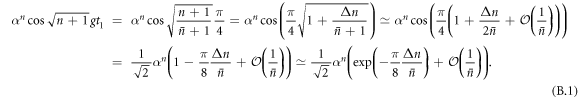
We have additionally used the trigonometric identity  and the small angle formulae
 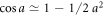 ,
,  . Substituting
  , and again working to
  , a little algebraic manipulation gives:
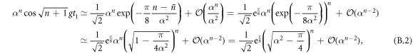
where we have used the approximation  , valid for small x. A similar treatment on the sine term in equation (17) produces

Putting these results back into equation (17) and taking into account normalization, the approximate state after interaction is thus given by equation (18).
Appendix C.: Derivation of evolution of the cavity state with subsequent interactions
We first note

where, for δ ≪ α', the second term may be neglected, while for  both remaining terms are
  . In each case it remains true that
  , and the analysis up to equation (B.1), used to find the atom-field state in equation (18), is unchanged. Note that for
  , the second term in equation (C.1) dominates, but as long as δ is small compared to α2,
  may still be considered to be small. Finally, note that for δ ≃ α2 then
  , and the approximations leading to equation (B.1) break down.
Assuming again for the moment therefore that  may be considered small, the atom-field state amplitudes following r interactions are found by repeating the analysis leading to equation (B.2), this time substituting
  as in equation (C.1):
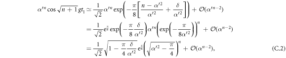
where use has again been made of the approximation  , valid for small x. As previously, a similar treatment produces

The approximate state after r interactions is then given by equation (21).
Appendix D.: Squeezed initial states
As briefly discussed in section 5.1, figure 5 indicates that the increase in success probabilities is greater than that expected from the increased photon number alone. An analysis of the distribution widths suggests that amplitude squeezing may account for this further discrepancy. We indeed find that the success probability of a squeezed state can be higher than that of a coherent state with equal mean photon number. Consider a quadrature squeezed state

with

For a state with  , the positivity of the squeezing parameter ζ corresponds to a reduction in the number uncertainty. Figure D1 shows the probability of the atom ending in the state
  when using such a cavity state as a function of the squeezing parameter ζ. For a mean photon number of 100.5, the maximal success probability with such a squeezed state is
  : this is far above the value obtained when the the cavity field is re-used in the second interaction step. The effect of squeezing, together with growing photon numbers, therefore suffices to explain the observed increase of success probabilities as discussed in 5.1.

Figure D1. Probability of measuring the atom in the state  after one atom-field interaction with the cavity initially being in a q-quadrature squeezed state with mean photon number
  , as a function of the squeezing parameter ζ. The dashed line shows the probability without squeezing.
Download figure:
Standard image High-resolution imageAt the limit of small squeezing parameter ζ, we can approximate the photon distribution of an amplitude squeezed state by a Gaussian number distribution with reduced width [59]:

Following this, the analytic approximation of the success probability is given by

which has a maximum of 1 − π/ at
at  when omitting higher order terms.
Footnotes
- 1
One must be careful not to confuse the resource theory of coherence with the thermodynamic resource theory in which coherence is only one type of resource. While in thermodynamics, only Gibbs (thermal) states are considered free, in coherence resource theory all incoherent states, including pure energy eigenstates, are free.
- 2
Even though the number of subsystems that exhibit coherence can be increased indefinitely, the overall coherence must stay constant.
- 3
Rather than
 , one could instead choose the interaction time defined by without changing the probabilities to first order.
 - 4
Note that we are neglecting the change in α' in subsequent rounds: as δ changes α' does also. However, it remains the same order of magnitude throughout as we are considering
. - 5
The width of the distribution is increased with respect to the initial coherent state with average photon number
, but is smaller than that of the coherent state with updated average photon number .


