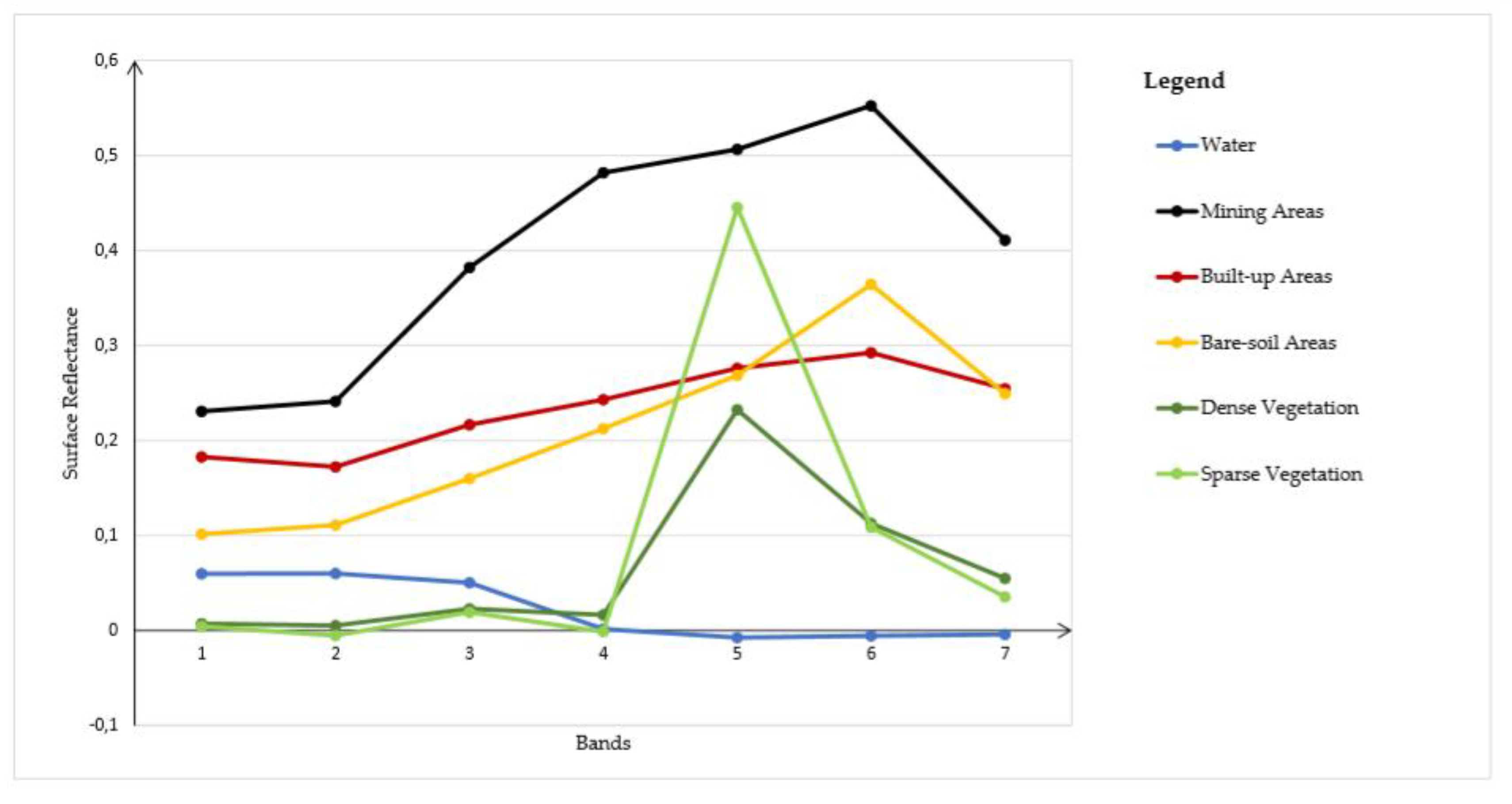
Figure 2.
Spectral signature of each class detected in the study area. The x and y axes report the original Landsat bands (Landsat 7 - Enhanced Thematic Mapper Plus (ETM+) and the surface reflectance, respectively, where 1 is band 1 (blue), 2 is band 2 (green), 3 is band 3 (red), 4 is band 4 (near infrared), 5 is band 5 (shortwave infrared 1), 6 is band 6 (thermal infrared), and 7 is band 7 (shortwave infrared 2).
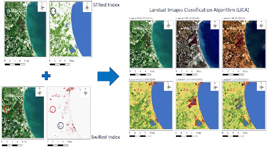
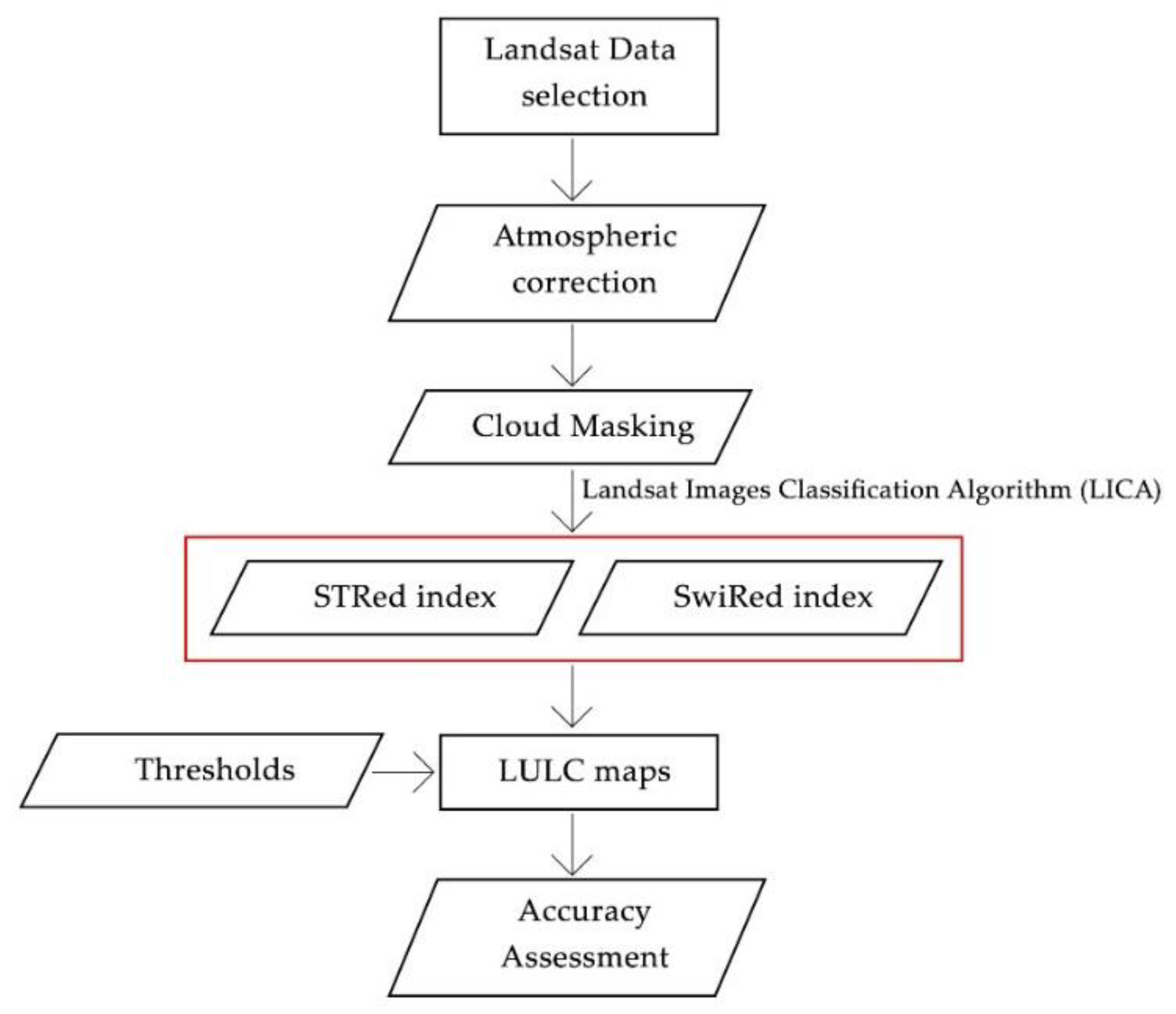
Figure 3.
Landsat Images Classification Algorithm (LICA) classification workflow.
Figure 3.
Landsat Images Classification Algorithm (LICA) classification workflow.
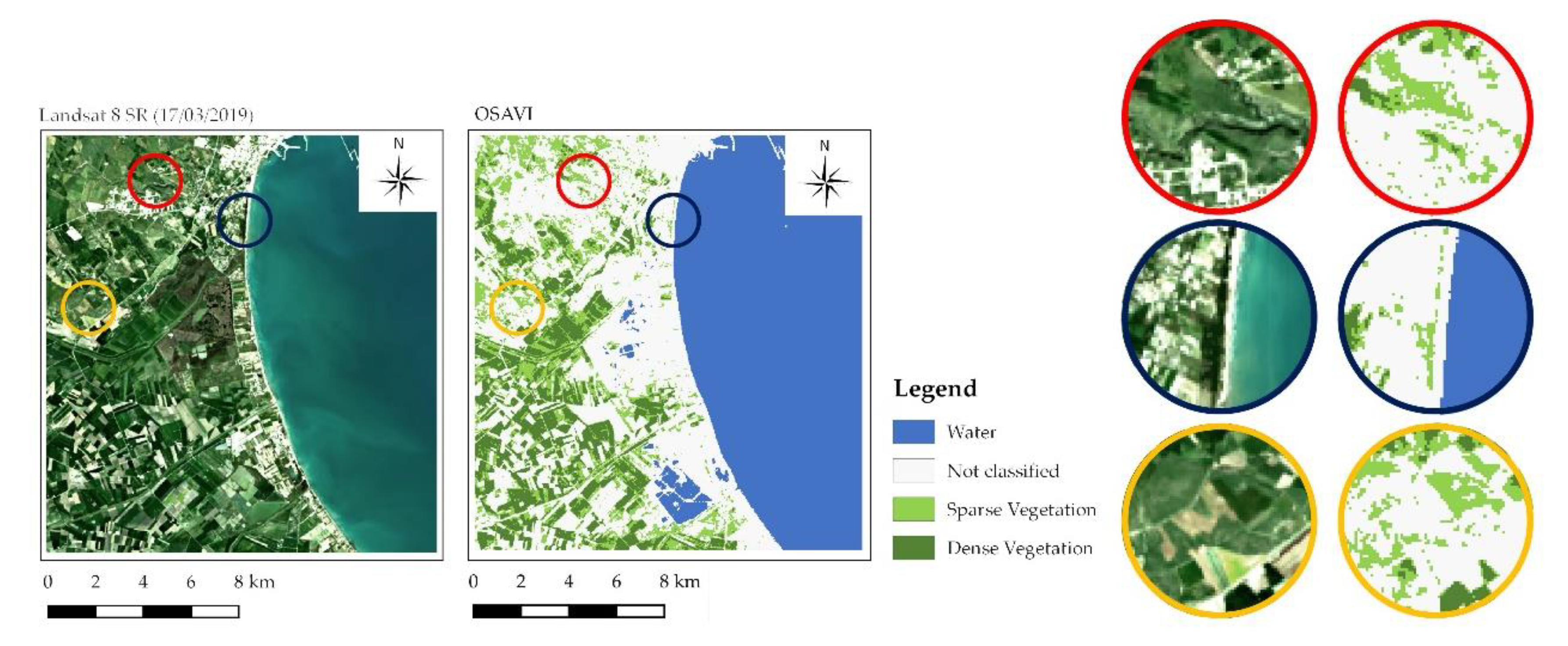
Figure 4.
Optimized Soil Adjusted Vegetation Index (OSAVI) classification outcome for Landsat 8 (image acquired on 17 March 2019). On the right, zoomed images with some misclassifications.
Figure 4.
Optimized Soil Adjusted Vegetation Index (OSAVI) classification outcome for Landsat 8 (image acquired on 17 March 2019). On the right, zoomed images with some misclassifications.
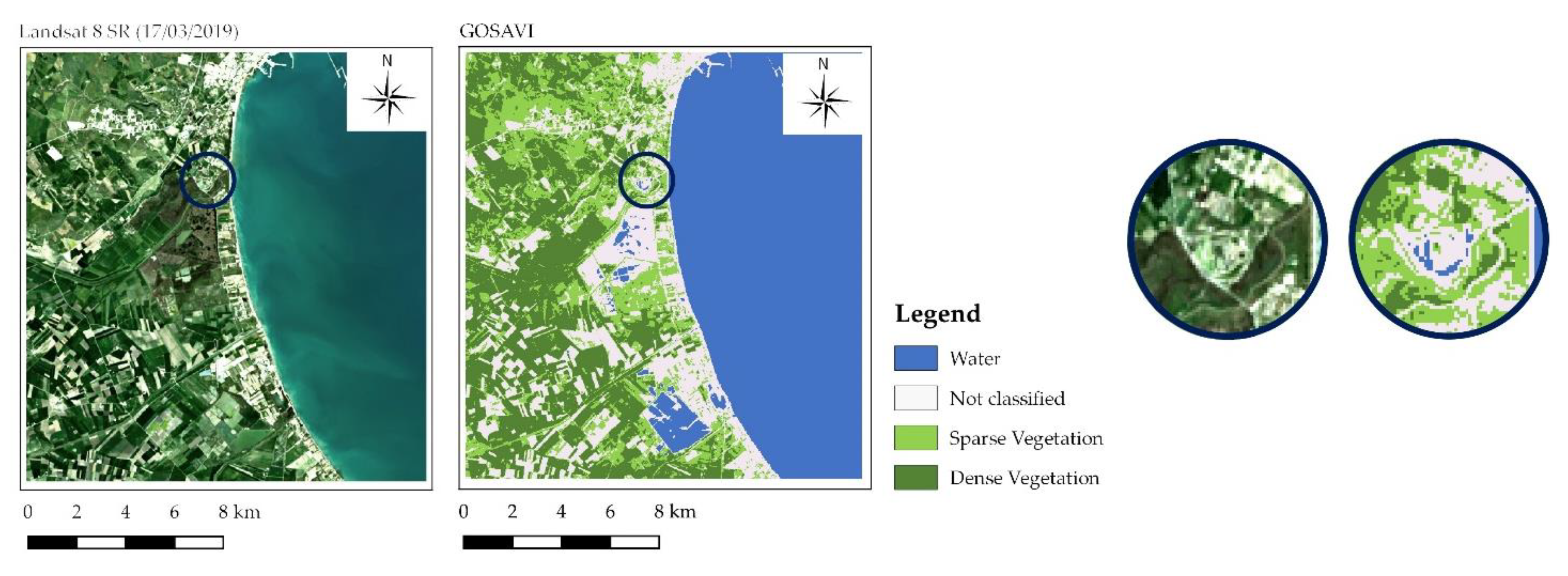
Figure 5.
Green Optimized Soil Adjusted Vegetation Index (GOSAVI) classification outcome for Landsat 8 (image acquired on 17 March 2019). On the right, zoomed images with some misclassifications.
Figure 5.
Green Optimized Soil Adjusted Vegetation Index (GOSAVI) classification outcome for Landsat 8 (image acquired on 17 March 2019). On the right, zoomed images with some misclassifications.
Figure 6.
Normalized Difference Bareness Index 2 (NDBaI2) classification outcome for Landsat 8 (image acquired on 17 March 2019). On the right, zoomed images with some misclassifications.
Figure 6.
Normalized Difference Bareness Index 2 (NDBaI2) classification outcome for Landsat 8 (image acquired on 17 March 2019). On the right, zoomed images with some misclassifications.
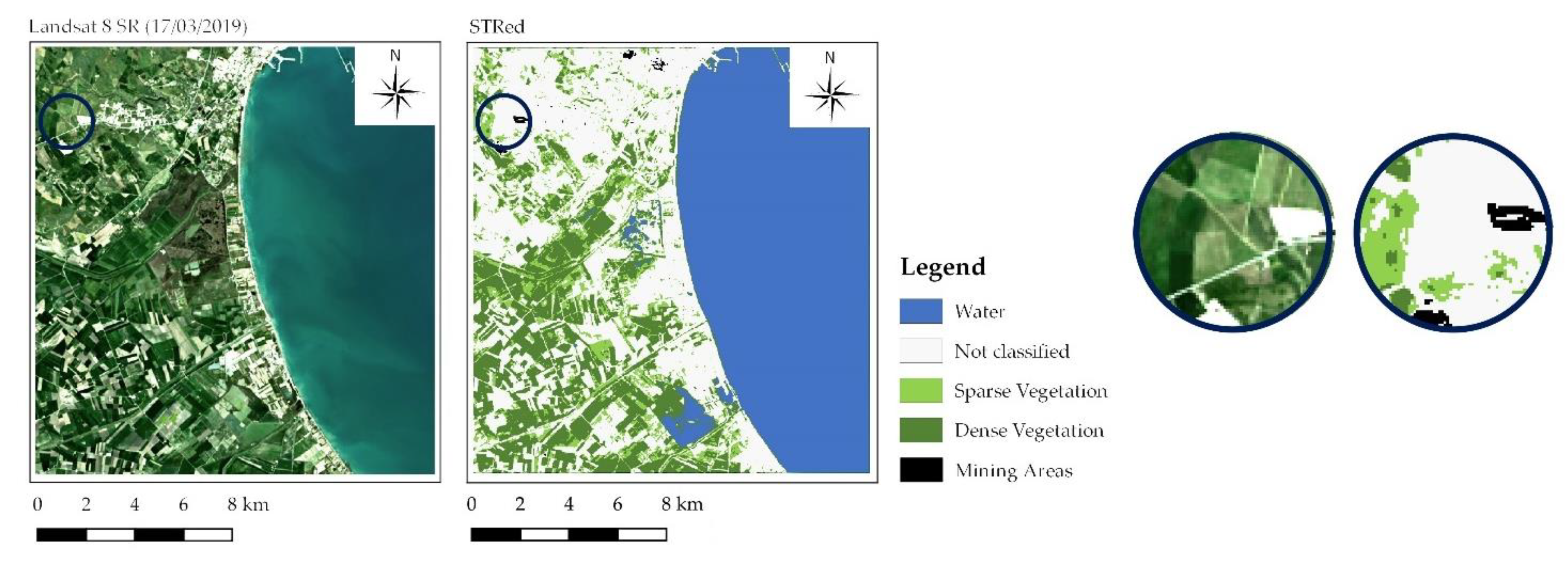
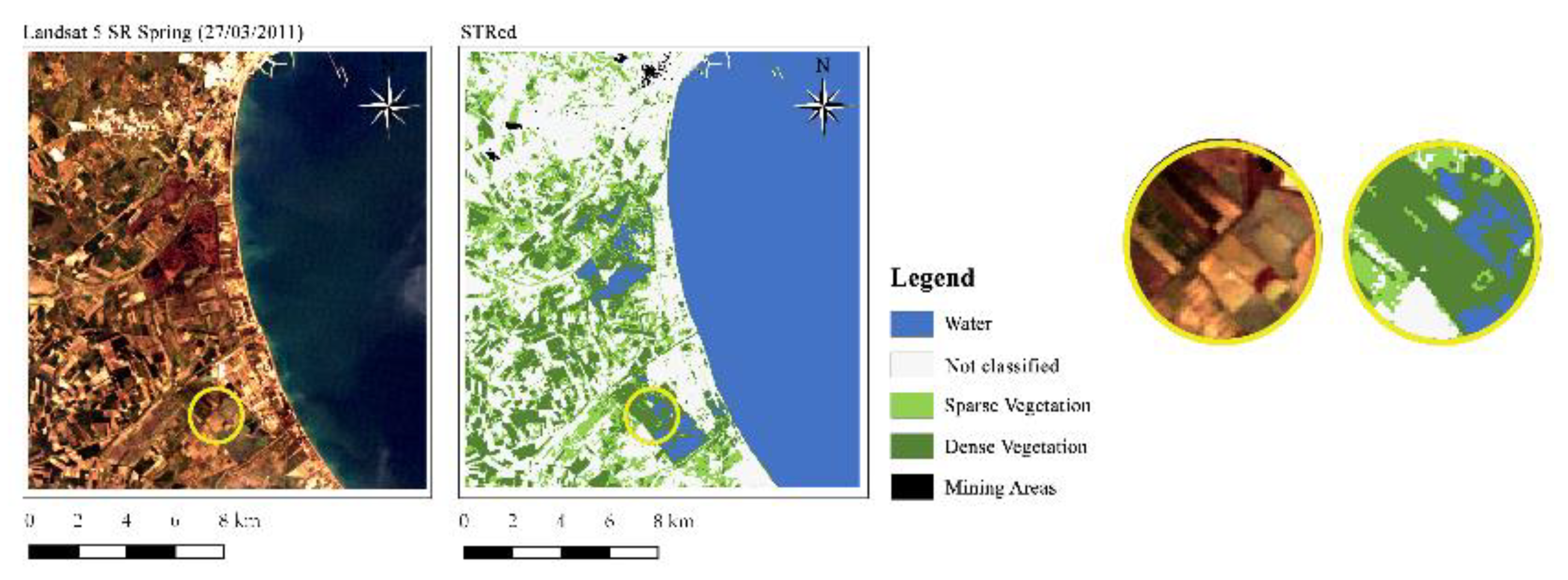
Figure 7.
SwirTiRed index (STRed) classification outcome for Landsat 5 (image acquired on 27 March 2011). On the right, zoomed images with some misclassifications.
Figure 7.
SwirTiRed index (STRed) classification outcome for Landsat 5 (image acquired on 27 March 2011). On the right, zoomed images with some misclassifications.
Figure 8.
SwirTiRed index (STRed) classification outcome for Landsat 5 (image acquired on 5 October 2011). On the right, zoomed images with some misclassifications.
Figure 8.
SwirTiRed index (STRed) classification outcome for Landsat 5 (image acquired on 5 October 2011). On the right, zoomed images with some misclassifications.
Figure 9.
SwirTiRed index (STRed) classification outcome for Landsat 7 (image acquired on 14 April 2003). On the right, zoomed images with some misclassifications.
Figure 9.
SwirTiRed index (STRed) classification outcome for Landsat 7 (image acquired on 14 April 2003). On the right, zoomed images with some misclassifications.
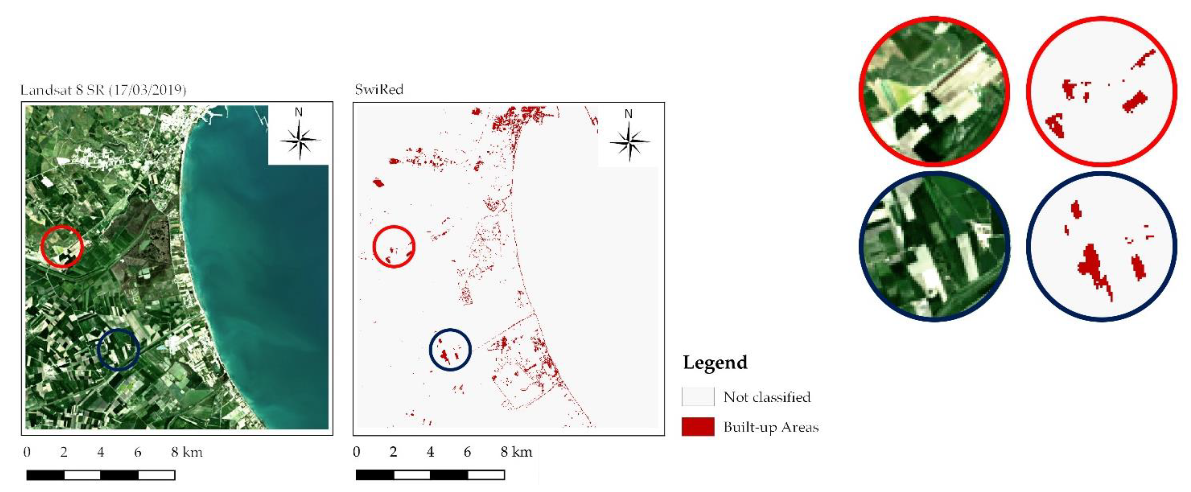
Figure 10.
SwiRed index (SwiRed) classification outcome for Landsat 8 (image acquired on 17 March 2019). On the right, zoomed images with some misclassifications.
Figure 10.
SwiRed index (SwiRed) classification outcome for Landsat 8 (image acquired on 17 March 2019). On the right, zoomed images with some misclassifications.
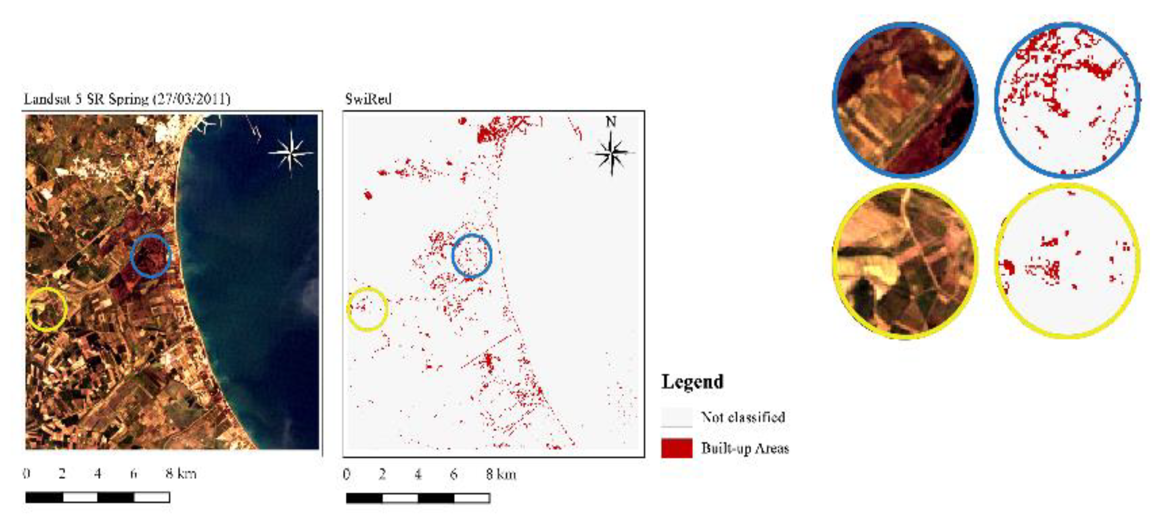
Figure 11.
SwiRed index (SwiRed) classification outcome for Landsat 5 (image acquired on 5 October 2011). On the right, zoomed images with some misclassifications.
Figure 11.
SwiRed index (SwiRed) classification outcome for Landsat 5 (image acquired on 5 October 2011). On the right, zoomed images with some misclassifications.
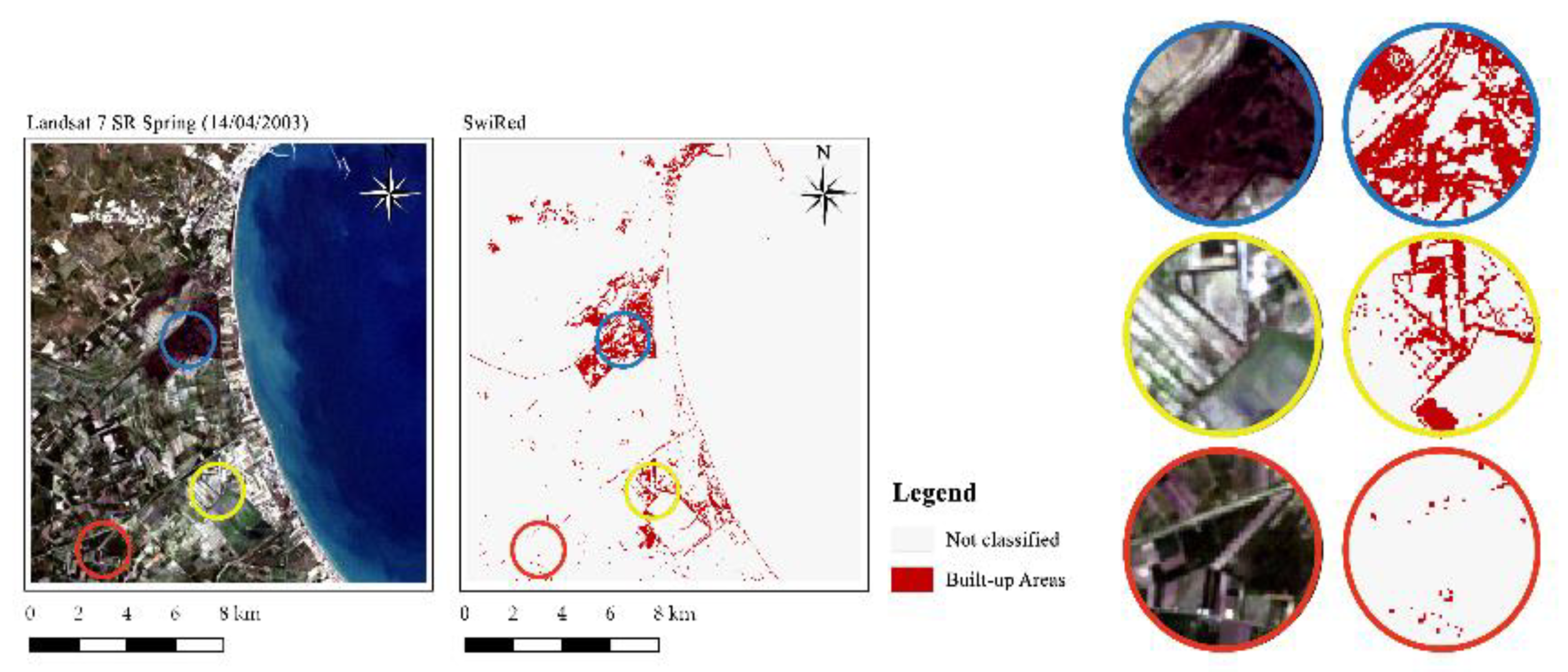
Figure 12.
SwiRed index (SwiRed) classification outcome for Landsat 7 (image acquired on 14 April 2003). On the right, zoomed images with some misclassifications.
Figure 12.
SwiRed index (SwiRed) classification outcome for Landsat 7 (image acquired on 14 April 2003). On the right, zoomed images with some misclassifications.
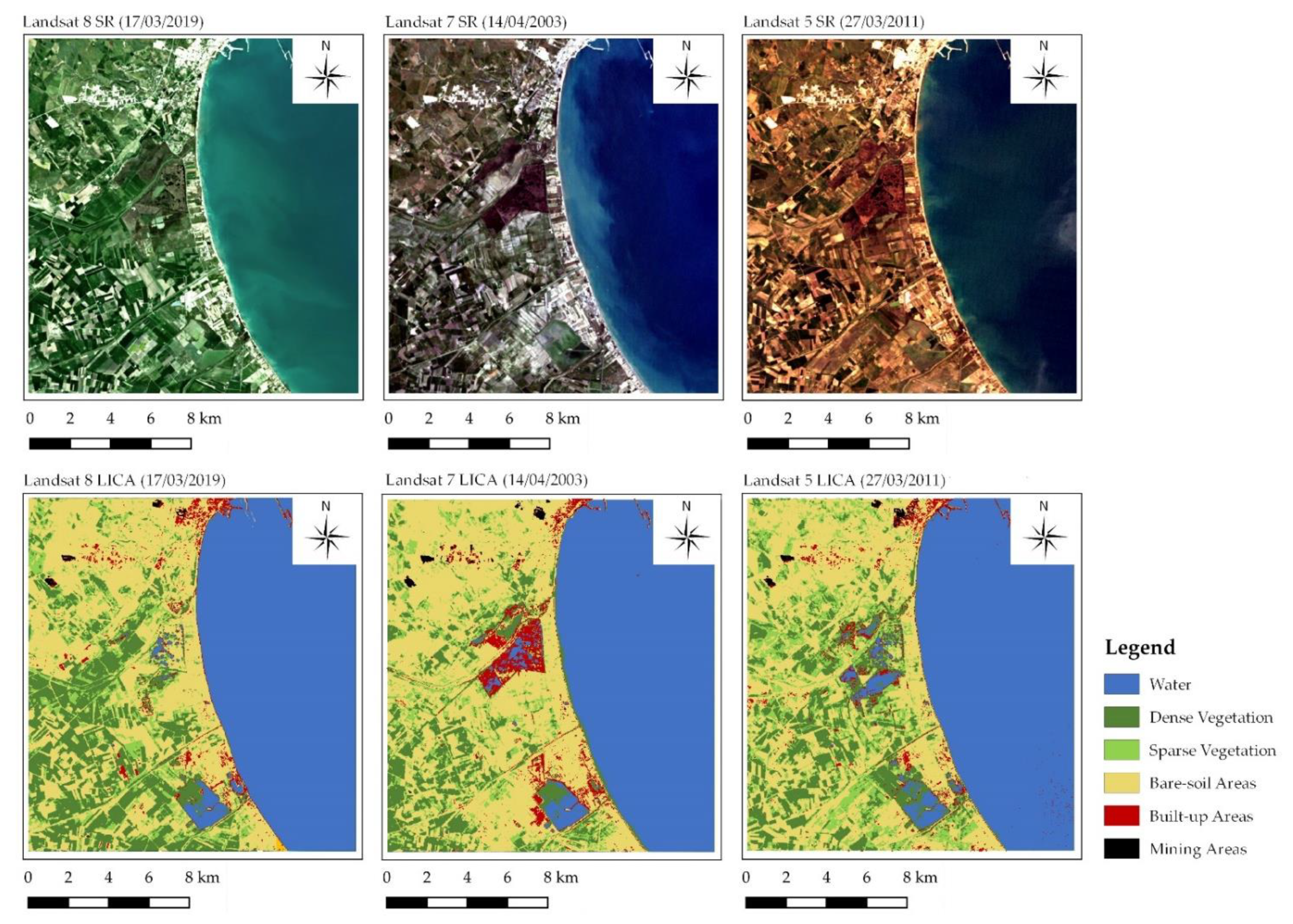
Figure 13.
Landsat Images Classification Algorithm (LICA) classification outcome for Landsat 8 (image acquired on 17 March 2019), Landsat 7 (image acquired on 6 April 2003), Landsat 5 (image acquired on 27 March 2011).
Figure 13.
Landsat Images Classification Algorithm (LICA) classification outcome for Landsat 8 (image acquired on 17 March 2019), Landsat 7 (image acquired on 6 April 2003), Landsat 5 (image acquired on 27 March 2011).
Table 1.
Main commonly used classification indices listed in alphabetical order. Indices in bold show the best performance. LC/LU column describes the land cover/land use classes detected from each index. OA column reports the best overall accuracy of each index. LC/LU, land cover/land use; OA: overall accuracy; W, water; DV, dense vegetation; SV, sparse vegetation; MA, mining areas; BS, bare soil; BUA: built-up area; *, water mask is required; -:, no classes were detected.
| Spectral Index | Citation | LC/LU | OA (%) |
|---|
| Aerosol Free Vegetation Index version 1.6 (AFRI1.6) | [60] | DV, SV | 72.24 |
| Aerosol Free Vegetation Index version 2.1 (AFRI2.1) | [60] | DV, SV | 86.02 |
| Atmospherically resistant vegetation index (ARVI) | [61] | W, DV, SV, BUA, BS | 59.97 |
| Adjusted Soil Brightness Index (ASBI) * | [62] | DV, SV | 66.70 |
| Ashburn Vegetation Index (AVI) | [63] | W | 99.78 |
| Automated Water Extraction Index (AWEI) | [64] | W, DV, SV, BUA, MA, BS | 68.04 |
| Automated Water Extraction Index (shadow version) (AWEIsh) | [64] | W, BUA | 91.46 |
| Build-area extraction index (BAEI) * | [65] | DV, SV, BUA | 63.60 |
| Biophysical Composition Index (BCI) | [66] | W, DV, SV | 68.23 |
| Built-up Land Features Extraction Index (BLFEI) | [67] | W, DV, SV, BUA, BS | 72.03 |
| Bare Soil Index (BSI) * | [68] | DV, SV | 73.62 |
| Built-up land (BUI) | [69] | W, DV, SV | 69.81 |
| Combinational Biophysical Composition Index (CBCI) | [70] | DV, SV | 67.22 |
| Green Chlorophyll Index (CI) | [71] | W, DV, SV | 68.40 |
| Davies-Bouldin index (DBI) | [72] | W, DV, SV, BUA, BS | 70.59 |
| Dry Bare-Soil Index (DBSI) * | [73] | DV, SV | 68.47 |
| Simple Difference Indices (DVI) | [74] | W, DV, SV | 69.85 |
| Enhanced Built-up and Bareness Index (EBBI) | [75] | W, DV, SV | 64.93 |
| Enhanced Normalized Difference Impervious Surfaces Index (ENDISI) | [76] | DV, SV BUA, MA | 67.55 |
| Enhanced Vegetation Index (EVI) | [77] | W, DV, SV, BUA, BS | 58.59 |
| Green Atmospherically Resistant Vegetation Index (GARI) | [78] | W, DV, SV, BUA, BS | 69.78 |
| “Ghost cities” Index (GCI) | [79] | W, DV, SV, BUA, BS | 71.26 |
| Green Difference Vegetation Index (GDVI) | [80] | W, DV, SV | 70.59 |
| Global Environment Monitoring Index (GEMI) | [81] | W, DV, SV | 67.74 |
| Green leaf index (GLI) | [82] | DV, SV | 66.70 |
| Green Normalized Difference Vegetation Index (GNDVI) | [78] | W, DV, SV, BUA, BS | 72.48 |
| Green Optimized Soil Adjusted Vegetation Index (GOSAVI) | [53] | W, DV, SV | 89.89 |
| Green-Red Vegetation Index (GRVI) | [83] | W, DV, SV, BUA, BS | 71.26 |
| Green Soil Adjusted Vegetation Index (GSAVI) | [53] | W, DV, SV, BUA, BS | 73.91 |
| Green Vegetation Index (GVI) * | [84] | DV, SV, BUA | 57.30 |
| Built-up Index (IBI) | [85] | DV, SV | 74.75 |
| Infrared Percentage Vegetation Index (IPVI) | [86] | W, DV, SV, BUA, BS | 69.10 |
| Modified Bare Soil Index (MBSI) | [70] | W, DV, SV | 73.22 |
| Modified Chlorophyll Absorption Ratio Index1 (MCARI1) | [87] | DV, SV | 64.28 |
| Modified Chlorophyll Absorption Ratio Index (MCARI2) | [87] | W, DV, SV, BUA, BS | 82.24 |
| MERIS Global Vegetation Index (MGVI) | [88] | W, DV, SV | 76.88 |
| Modification of Normalized Difference Snow Index (MNDSI) | [89] | W, MA | 76.55 |
| Modification of normalized difference water index (MNDWI) | [90] | W, BUA | 74.62 |
| Modified Nonlinear Vegetation Index (MNLI) | [91] | W, DV, SV | 77.40 |
| Modified Soil Adjusted Vegetation Index 2 (MSAVI2) | [92] | W, DV, SV, BUA, BS | 83.30 |
| Misra Soil Brightness Index (MSBI) | [93] | W, DV, SV, BUA, BS | 78.56 |
| Modified Simple Ratio (MSR) | [94] | W, DV, SV, BUA, BS | 67.03 |
| Misra Yellow Vegetation Index (MYVI) | [93] | - | - |
| New Built-up Index (NBI) * | [95] | DV, SV, BUA, MA, BS | 71.46 |
| Normalized Difference Bare Land Index (NBLI) * | [96] | DV, SV, BUA, MA, BS | 75.51 |
| New Built-up Index (NBUI) | [97] | W, DV, SV | 76.39 |
| Normalized Canopy Index (NCI) | [98] | W, BUA | 78.34 |
| Normalized Difference Bareness Index (NDBaI) | [54] | W, DV, SV, BUA, MA, BS | 67.93 |
| Normalized Difference Bareness Index (version 2) (NDBaI2) | [54] | W, DV, SV, BUA, MA, BS | 82.59 |
| Normalized Difference Built-up Index (NDBI) | [99] | DV, SV | 71.14 |
| Normalized Difference Impervious Surface Index (NDISI) | [100] | W, MA | 97.60 |
| Normalized Difference Moisture Index (NDMI) * | [101] | DV, SV | 73.47 |
| Normalized Difference Tillage Index (NDTI) * | [102] | DV, SV | 71.57 |
| Normalized Difference Vegetation Index (NDVI) | [56] | W, DV, SV, BUA, BS | 73.24 |
| Normalized Difference Water Index (NDWI) | [103] | W, DV, SV, BUA, BS | 73.54 |
| Non-Linear Index (NLI) | [104] | W, DV, SV | 76.63 |
| Optimized Soil Adjusted Vegetation Index (OSAVI) | [52] | W, DV, SV | 88.84 |
| Renormalized Difference Vegetation Index (RDVI) | [105] | W, DV, SV | 77.34 |
| Ratio Vegetation Index (RVI) | [106] | W, DV, SV, BUA, BS | 72.30 |
| Soil-Adjusted Vegetation Index (SAVI) | [107] | W, DV, SV | 72.04 |
| Soil Brightness Index (SBI) | [108] | W, BUA, MA | 80.27 |
| Specific Leaf Area Vegetation Index (SLAVI) | [109] | W, DV, SV | 83.56 |
| Simple Ratio (SR) | [110] | W, DV, SV | 68.93 |
| Transformed difference vegetation index (TDVI) | [111] | W | 99.81 |
| Triangular Greenness Index (TGI) | [112] | - | - |
| Triangular Vegetation Index (TVI) | [113] | W, DV, SV | 74.15 |
| Urban Index (UI) | [114] | BUA | 76.66 |
| Visible Atmospherically Resistant Index (VARI) | [115] | W, DV, SV | 68.34 |
| Visible-Band Difference Vegetation Index (VDVI) | [116] | DV, SV | 66.70 |
| Vegetation Index of Biotic Integrity (VIBI) | [117] | DV, SV | 66.57 |
| Wide Dynamic Range Vegetation Index (WDRVI) | [118] | W, DV, SV | 78.87 |
| Water index 2015 (WI2015) | [119] | W | 99.81 |
| Worldview Improved Vegetative Index (WV-VI) | [120] | W, DV, SV, BUA, BS | 75.47 |
| Yellow Stuff Index (YVI) * | [121] | DV, SV | 66.70 |
Table 2.
Range value of LICA to extract the different land cover classes.
Table 2.
Range value of LICA to extract the different land cover classes.
| Land Cover Class | Range value (SwiRed) |
| Built- up areas | 0 < value < 0.22 |
| Land Cover Class | Range value (STRed) |
| Water | value < −0.5 |
| Dense vegetation | −0.05 < value < −0.07 |
| Sparse vegetation | 0.07 < value < 0.00 |
| Mining areas | Value > 0.45 |
Table 3.
Selected Landsat data description. ETM+, enhanced thematic mapper; TM, thematic mapper; OLI-TIRS, operational land imager - thermal infrared.
Table 3.
Selected Landsat data description. ETM+, enhanced thematic mapper; TM, thematic mapper; OLI-TIRS, operational land imager - thermal infrared.
| ID | Landsat Satellite Mission | Sensor | Landsat Images | Acquisition Date | Average Cloud Cover (%) |
|---|
| 1 | Landsat 7 | ETM+ | LE07_L1TP_188031_20020121_20170213 | 21 January 2002 | 4 |
| 2 | LE07_L1TP_188031_20020801_20170213 | 01 August 2002 | 6 |
| 3 | LE07_L1TP_189031_2002127_20170128 | 27 October 2002 | 1 |
| 4 | LE07_L1TP_188031_20030414_20170126 | 14 April 2003 | 4 |
| 1 | Landsat 5 | TM | LT05_L1TP_188031_20110207_20161010 | 07 February 2011 | 1 |
| 2 | LT05_L1TP_188031_20110327_20161209 | 27 March 2011 | 16 |
| 3 | LT05_L1TP_189031_20110825_20161008 | 25 August 2011 | 0 |
| 4 | LT05_L1TP_188031_20111005_20161005 | 05 October 2011 | 1 |
| 1 | Landsat 8 | OLI-TIRS | LC08_L1TP_188031_20171208_20171223 | 08 December 2017 | 1.69 |
| 2 | LC08_L1TP_189031_20180812_20180815 | 12 August 2018 | 8.1 |
| 3 | LC08_L1TP_188031_20180922_20180928 | 22 September 2018 | 2.41 |
| 4 | LC08_L1TP_188031_20190925_201911017 | 17 March 2019 | 19.46 |
Table 4.
OA, PA, and UA obtained through the application of Optimized Soil Adjusted Vegetation Index (OSAVI) on the data acquired by Landsat 7 mission. UA, user’s accuracy; PA, producer’s accuracy; OA, overall accuracy.
Table 4.
OA, PA, and UA obtained through the application of Optimized Soil Adjusted Vegetation Index (OSAVI) on the data acquired by Landsat 7 mission. UA, user’s accuracy; PA, producer’s accuracy; OA, overall accuracy.
| | L7—21 January 2002 | L7—14 April 2003 | L7—01 August 2002 | L7—27 October 2002 |
|---|
| Land Cover Class | PA (%) | UA (%) | PA (%) | UA (%) | PA (%) | UA (%) | PA (%) | UA (%) |
|---|
| Water | 95.79 | 100.00 | 95.04 | 100.00 | 90.11 | 98.99 | 95.60 | 99.24 |
| Dense Vegetation | 79.57 | 87.40 | 72.38 | 86.21 | 70.97 | 98.05 | 95.56 | 45.84 |
| Sparse Vegetation | 73.89 | 89.78 | 90.55 | 81.91 | 25.14 | 33.96 | 49.30 | 67.03 |
| Not classified | 100.00 | 78.38 | 100.00 | 92.28 | 91.13 | 62.43 | 79.47 | 98.17 |
| Mining Areas | / | / | / | / | / | / | / | / |
| Bare Soil | / | / | / | / | / | / | / | / |
| Built-up areas | / | / | / | / | / | / | / | / |
| OA (%) | 87.83 | 88.84 | 74.02 | 78.23 |
Table 5.
OA, PA, and UA obtained through the application of Optimized Soil Adjusted Vegetation Index (OSAVI) on the data acquired by Landsat 5 mission. UA, user’s accuracy; PA, producer’s accuracy; OA, overall accuracy.
Table 5.
OA, PA, and UA obtained through the application of Optimized Soil Adjusted Vegetation Index (OSAVI) on the data acquired by Landsat 5 mission. UA, user’s accuracy; PA, producer’s accuracy; OA, overall accuracy.
| | L5—07 February 2011 | L5—27 March 2011 | L5—25 August 2011 | L5—05 October 2011 |
|---|
| Land Cover Class | PA (%) | UA (%) | PA (%) | UA (%) | PA (%) | UA (%) | PA (%) | UA (%) |
|---|
| Water | 95.05 | 93.35 | 89.73 | 100.00 | 90.30 | 99.05 | 66.30 | 96.02 |
| Dense Vegetation | 64.16 | 53.27 | 66.49 | 78.44 | 48.54 | 93.55 | 80.54 | 69.00 |
| Sparse Vegetation | 35.36 | 58.67 | 76.25 | 81.06 | 43.05 | 51.90 | 67.92 | 80.36 |
| Not classified | 92.21 | 70.75 | 100.00 | 71.88 | 81.90 | 40.89 | 93.83 | 72.77 |
| Mining Areas | / | / | / | / | / | / | / | / |
| Bare Soil | / | / | / | / | / | / | / | / |
| Built-up areas | / | / | / | / | / | / | / | / |
| OA (%) | 68.71 | 84.84 | 72.44 | 77.98 |
Table 6.
OA, PA, and UA obtained through the application of Optimized Soil Adjusted Vegetation Index (OSAVI) on the data acquired by Landsat 8 mission. UA, user’s accuracy; PA, producer’s accuracy; OA, overall accuracy.
Table 6.
OA, PA, and UA obtained through the application of Optimized Soil Adjusted Vegetation Index (OSAVI) on the data acquired by Landsat 8 mission. UA, user’s accuracy; PA, producer’s accuracy; OA, overall accuracy.
| | L8—08 December 2008 | L8—12 August 2018 | L8—22 September 2018 | L8—17 March 2019 |
|---|
| Land Cover Class | PA (%) | UA (%) | PA (%) | UA (%) | PA (%) | UA (%) | PA (%) | UA (%) |
|---|
| Water | 99.13 | 100.00 | 98.19 | 99.85 | 89.01 | 99.53 | 97.30 | 100.00 |
| Dense Vegetation | 76.93 | 75.39 | 59.09 | 91.95 | 86.49 | 96.60 | 80.85 | 73.47 |
| Sparse Vegetation | 22.91 | 52.00 | 27.34 | 51.27 | 81.74 | 82.82 | 55.04 | 71.57 |
| Not classified | 99.46 | 70.60 | 99.81 | 65.33 | 93.98 | 83.79 | 100.00 | 79.54 |
| Mining Areas | / | / | / | / | / | / | / | / |
| Bare Soil | / | / | / | / | / | / | / | / |
| Built-up areas | / | / | / | / | / | / | / | / |
| OA (%) | 81.41 | 81.00 | 88.91 | 83.56 |
Table 7.
OA, PA, and UA obtained through the application of Green Optimized Soil Adjusted Vegetation Index (GOSAVI) on the data acquired by Landsat 7 mission. UA, user’s accuracy; PA, producer’s accuracy; OA, overall accuracy.
Table 7.
OA, PA, and UA obtained through the application of Green Optimized Soil Adjusted Vegetation Index (GOSAVI) on the data acquired by Landsat 7 mission. UA, user’s accuracy; PA, producer’s accuracy; OA, overall accuracy.
| | L7—21 January 2002 | L7—14 April 2003 | L7—01 August 2002 | L7—27 October 2002 |
|---|
| Land Cover Class | PA (%) | UA (%) | PA (%) | UA (%) | PA (%) | UA (%) | PA (%) | UA (%) |
|---|
| Water | 96.34 | 100.00 | 96.70 | 100.00 | 86.26 | 100.00 | 96.15 | 97.22 |
| Dense Vegetation | 60.57 | 88.48 | 70.22 | 91.18 | 70.97 | 93.12 | 86.69 | 44.79 |
| Sparse Vegetation | 65.78 | 83.83 | 94.67 | 76.05 | 18.23 | 39.05 | 52.09 | 71.39 |
| Not classified | 100.00 | 70.57 | 89.16 | 95.52 | 97.21 | 59.50 | 83.09 | 97.50 |
| Mining Areas | / | / | / | / | / | / | / | / |
| Bare Soil | / | / | / | / | / | / | / | / |
| Built-up areas | / | / | / | / | / | / | / | / |
| OA (%) | 82.86 | 87.74 | 73.57 | 79.12 |
Table 8.
OA, PA, and UA obtained through the application of Green Optimized Soil Adjusted Vegetation Index (GOSAVI) on the data acquired by Landsat 5 mission. UA, user’s accuracy; PA, producer’s accuracy; OA, overall accuracy.
Table 8.
OA, PA, and UA obtained through the application of Green Optimized Soil Adjusted Vegetation Index (GOSAVI) on the data acquired by Landsat 5 mission. UA, user’s accuracy; PA, producer’s accuracy; OA, overall accuracy.
| | L5—07 February 2011 | L5—March 27 2011 | L5—25 August 2011 | L5—05 October 2011 |
|---|
| Land Cover Class | PA (%) | UA (%) | PA (%) | UA (%) | PA (%) | UA (%) | PA (%) | UA (%) |
|---|
| Water | 94.32 | 100.00 | 95.73 | 100.00 | 93.56 | 58.46 | 74.91 | 97.61 |
| Dense Vegetation | 60.04 | 43.51 | 63.98 | 88.15 | 52.30 | 89.29 | 81.71 | 54.40 |
| Sparse Vegetation | 25.03 | 35.39 | 89.31 | 81.74 | 43.05 | 40.25 | 59.62 | 85.87 |
| Not classified | 59.51 | 52.17 | 99.58 | 100.00 | 90.26 | 43.90 | 95.41 | 77.60 |
| Mining Areas | / | / | / | / | / | / | / | / |
| Bare Soil | / | / | / | / | / | / | / | / |
| Built-up areas | / | / | / | / | / | / | / | / |
| OA (%) | 55.22 | 89.89 | 76.37 | 78.82 |
Table 9.
OA, PA, and UA obtained through the application of Green Optimized Soil Adjusted Vegetation Index (GOSAVI) on the data acquired by Landsat 8 mission. UA, user’s accuracy; PA, producer’s accuracy; OA, overall accuracy.
Table 9.
OA, PA, and UA obtained through the application of Green Optimized Soil Adjusted Vegetation Index (GOSAVI) on the data acquired by Landsat 8 mission. UA, user’s accuracy; PA, producer’s accuracy; OA, overall accuracy.
| | L8—08 December 2008 | L8—12 August 2018 | L8—22 September 2018 | L8—17 March 2019 |
|---|
| Land Cover Class | PA (%) | UA (%) | PA (%) | UA (%) | PA (%) | UA (%) | PA (%) | UA (%) |
|---|
| Water | 99.49 | 100.00 | 98.19 | 100.00 | 90.84 | 98.41 | 99.81 | 100.00 |
| Dense Vegetation | 75.62 | 75.29 | 59.72 | 89.02 | 84.80 | 89.64 | 92.88 | 63.74 |
| Sparse Vegetation | 40.50 | 24.23 | 25.20 | 43.56 | 75.00 | 87.34 | 17.94 | 61.86 |
| Not classified | 99.46 | 66.95 | 100.00 | 66.31 | 97.95 | 84.62 | 100.00 | 99.74 |
| Mining Areas | / | / | / | / | / | / | / | / |
| Bare Soil | / | / | / | / | / | / | / | / |
| Built-up areas | / | / | / | / | / | / | / | / |
| OA (%) | 79.32 | 80.89 | 89.15 | 80.35 |
Table 10.
OA, PA, and UA obtained through the application of Normalized Difference Bareness Index (version 2) (NDBIaI2) on the data acquired by Landsat 7 mission. UA, user’s accuracy; PA, producer’s accuracy; OA, overall accuracy.
Table 10.
OA, PA, and UA obtained through the application of Normalized Difference Bareness Index (version 2) (NDBIaI2) on the data acquired by Landsat 7 mission. UA, user’s accuracy; PA, producer’s accuracy; OA, overall accuracy.
| | L7—21 January 2002 | L7—14 April 2003 | L7—01 August 2002 | L7—27 October 2002 |
|---|
| Land Cover Class | PA (%) | UA (%) | PA (%) | UA (%) | PA (%) | UA (%) | PA (%) | UA (%) |
|---|
| Water | 95.24 | 100.00 | 97.07 | 100.00 | 87.55 | 100.00 | 95.24 | 100.00 |
| Dense Vegetation | 69.89 | 54.32 | 81.48 | 95.14 | 41.94 | 50.61 | 89.11 | 79.78 |
| Sparse Vegetation | 19.62 | 51.75 | 52.36 | 75.66 | 69.34 | 60.19 | 26.84 | 27.27 |
| Not classified | / | / | / | / | / | / | / | / |
| Mining Areas | 30.96 | 92.55 | 77.58 | 94.78 | 90.20 | 95.04 | 64.77 | 95.25 |
| Bare Soil | 94.35 | 63.88 | 87.17 | 62.54 | 91.33 | 79.71 | 69.31 | 64.17 |
| Built-up areas | 27.18 | 31.98 | 41.04 | 37.04 | 31.79 | 48.44 | 46.15 | 46.88 |
| OA (%) | 66.89 | 76.10 | 76.23 | 66.61 |
Table 11.
OA, PA, and UA obtained through the application of Normalized Difference Bareness Index (version 2) (NDBIaI2) on the data acquired by Landsat 5 mission. UA, user’s accuracy; PA, producer’s accuracy; OA, overall accuracy.
Table 11.
OA, PA, and UA obtained through the application of Normalized Difference Bareness Index (version 2) (NDBIaI2) on the data acquired by Landsat 5 mission. UA, user’s accuracy; PA, producer’s accuracy; OA, overall accuracy.
| | L5—07 February 2011 | L5—27 March 2011 | L5—25 August 2011 | L5—05 October 2011 |
|---|
| Land Cover Class | PA (%) | UA (%) | PA (%) | UA (%) | PA (%) | UA (%) | PA (%) | UA (%) |
|---|
| Water | 96.89 | 100.00 | 90.59 | 100.00 | 82.49 | 100.00 | 84.25 | 100.00 |
| Dense Vegetation | 86.56 | 53.91 | 74.73 | 73.42 | 62.97 | 45.47 | 53.70 | 54.55 |
| Sparse Vegetation | 54.76 | 84.42 | 38.24 | 65.05 | 78.63 | 78.63 | 48.11 | 57.41 |
| Not classified | / | / | / | / | / | / | / | / |
| Mining Areas | 56.86 | 99.32 | 86.27 | 98.65 | 84.71 | 99.08 | 82.56 | 97.89 |
| Bare Soil | 93.81 | 89.17 | 92.13 | 59.38 | 92.50 | 83.88 | 79.33 | 58.56 |
| Built-up areas | 28.21 | 26.19 | 16.92 | 31.43 | 42.82 | 38.66 | 34.87 | 45.26 |
| OA (%) | 78.95 | 75.07 | 80.28 | 61.55 |
Table 12.
OA, PA, and UA obtained through the application of Normalized Difference Bareness Index (version 2) (NDBIaI2) on the data acquired by Landsat 8 mission. UA: UA, user’s accuracy; PA, producer’s accuracy; OA, overall accuracy.
Table 12.
OA, PA, and UA obtained through the application of Normalized Difference Bareness Index (version 2) (NDBIaI2) on the data acquired by Landsat 8 mission. UA: UA, user’s accuracy; PA, producer’s accuracy; OA, overall accuracy.
| | L8—08 December 2008 | L8—12 August 2018 | L8—22 September 2018 | L8—17 March 2019 |
|---|
| Land Cover Class | PA (%) | UA (%) | PA (%) | UA (%) | PA (%) | UA (%) | PA (%) | UA (%) |
|---|
| Water | 98.55 | 100.00 | 100.00 | 99.93 | 93.77 | 99.03 | 96.72 | 100.00 |
| Dense Vegetation | 91.53 | 57.10 | 32.45 | 70.41 | 39.86 | 77.12 | 98.89 | 80.93 |
| Sparse Vegetation | 27.48 | 50.30 | 69.59 | 62.02 | 36.96 | 48.60 | 37.59 | 71.83 |
| Not classified | / | / | / | / | / | / | / | / |
| Mining Areas | 41.96 | 100.00 | 81.18 | 99.04 | 74.02 | 99.52 | 79.92 | 100.00 |
| Bare Soil | 93.72 | 87.34 | 93.36 | 80.67 | 88.88 | 32.16 | 30.14 | 39.25 |
| Built-up areas | 29.74 | 39.27 | 26.41 | 32.54 | 20.00 | 38.31 | 70.19 | 23.10 |
| OA (%) | 80.20 | 82.59 | 66.31 | 72.04 |
Table 13.
OA, PA, and UA obtained computing STRed on the images acquired by Landsat 7 mission. UA, user’s accuracy; PA, producer’s accuracy; OA, overall accuracy.
Table 13.
OA, PA, and UA obtained computing STRed on the images acquired by Landsat 7 mission. UA, user’s accuracy; PA, producer’s accuracy; OA, overall accuracy.
| | L7—21 January 2002 | L7—14 April 2003 | L7—01 August 2002 | L7—27 October 2002 |
|---|
| Land Cover Class | PA (%) | UA (%) | PA (%) | UA (%) | PA (%) | UA (%) | PA (%) | UA (%) |
|---|
| Water | 95.79 | 97.39 | 98.80 | 100.00 | 98.35 | 100.00 | 99.15 | 96.88 |
| Sparse Vegetation | 85.75 | 69.37 | 72.56 | 92.81 | 62.98 | 74.51 | 92.95 | 93.78 |
| Dense Vegetation | 76.76 | 54.57 | 98.66 | 89.84 | 75.65 | 69.52 | 84.08 | 76.41 |
| Mining areas | 81.57 | 100.00 | 75.11 | 99.41 | 97.65 | 88.25 | 46.44 | 97.18 |
| Not classified | 85.67 | 95.78 | 99.73 | 80.62 | 89.66 | 72.90 | 61.93 | 83.63 |
| OA (%) | 86.49 | 94.30 | 80.95 | 87.73 |
Table 14.
OA, PA, and UA obtained computing STRed on the images acquired by Landsat 5 mission. UA, user’s accuracy; PA, producer’s accuracy; OA, overall accuracy.
Table 14.
OA, PA, and UA obtained computing STRed on the images acquired by Landsat 5 mission. UA, user’s accuracy; PA, producer’s accuracy; OA, overall accuracy.
| | L5—07 February 2011 | L5—27 March 2011 | L5—25 August 2011 | L5—05 October 2011 |
|---|
| Land Cover Class | PA (%) | UA (%) | PA (%) | UA (%) | PA (%) | UA (%) | PA (%) | UA (%) |
|---|
| Water | 99.27 | 98.91 | 98.72 | 100.00 | 94.86 | 99.62 | 97.38 | 100.00 |
| Sparse Vegetation | 81.40 | 90.78 | 91.45 | 95.65 | 89.69 | 94.63 | 68.64 | 55.10 |
| Dense Vegetation | 80.11 | 80.54 | 98.31 | 91.26 | 84.94 | 78.99 | 96.04 | 82.20 |
| Mining areas | 69.80 | 99.44 | 98.67 | 99.11 | 87.45 | 100.00 | 94.22 | 99.53 |
| Not classified | 99.32 | 80.87 | 99.31 | 97.17 | 99.47 | 89.61 | 86.83 | 78.42 |
| OA (%) | 87.88 | 97.76 | 93.20 | 85.83 |
Table 15.
OA, PA, and UA obtained accuracy computing STRed on the images acquired by Landsat 8 mission. UA, user’s accuracy; PA, producer’s accuracy; OA, overall accuracy.
Table 15.
OA, PA, and UA obtained accuracy computing STRed on the images acquired by Landsat 8 mission. UA, user’s accuracy; PA, producer’s accuracy; OA, overall accuracy.
| | L8—08 December 2008 | L8—12 August 2018 | L8—22 September 2018 | L8—17 March 2019 |
|---|
| Land Cover Class | PA (%) | UA (%) | PA (%) | UA (%) | PA (%) | UA (%) | PA (%) | UA (%) |
|---|
| Water | 98.63 | 97.92 | 97.68 | 100.00 | 98.65 | 100.00 | 99.43 | 100.00 |
| Sparse Vegetation | 94.21 | 97.93 | 89.59 | 87.13 | 69.29 | 72.73 | 93.53 | 98.64 |
| Dense Vegetation | 86.28 | 92.92 | 73.01 | 74.72 | 73.74 | 86.13 | 99.17 | 93.93 |
| Mining areas | 84.51 | 96.53 | 82.75 | 98.60 | 61.56 | 100.00 | 98.22 | 97.79 |
| Not classified | 99.55 | 56.08 | 99.53 | 79.52 | 100.00 | 53.04 | 98.89 | 99.19 |
| OA (%) | 93.33 | 87.93 | 85.08 | 98.71 |
Table 16.
OA, PA, and UA obtained computing SwiRed index on the images acquired by Landsat 7 mission. UA, user’s accuracy; PA, producer’s accuracy; OA, overall accuracy.
Table 16.
OA, PA, and UA obtained computing SwiRed index on the images acquired by Landsat 7 mission. UA, user’s accuracy; PA, producer’s accuracy; OA, overall accuracy.
| | L7—21 January 2002 | L7—14 April 2003 | L7—01 August 2002 | L7—27 October 2002 |
|---|
| Land Cover Class | PA (%) | UA (%) | PA (%) | UA (%) | PA (%) | UA (%) | PA (%) | UA (%) |
|---|
| Built-up areas | 72.82 | 82.75 | 90.45 | 73.77 | 74.10 | 74.10 | 80.00 | 83.88 |
| Not classified | 98.27 | 96.05 | 93.88 | 89.07 | 97.88 | 97.32 | 97.55 | 97.20 |
| OA (%) | 91.31 | 89.28 | 92.77 | 94.30 |
Table 17.
OA, PA, and UA obtained computing SwiRed index on the images acquired by Landsat 5 mission. UA, user’s accuracy; PA, producer’s accuracy; OA, overall accuracy.
Table 17.
OA, PA, and UA obtained computing SwiRed index on the images acquired by Landsat 5 mission. UA, user’s accuracy; PA, producer’s accuracy; OA, overall accuracy.
| | L5—07 February 2011 | L5—27 March 2011 | L5—25 August 2011 | L5—05 October 2011 |
|---|
| Land Cover Class | PA (%) | UA (%) | PA (%) | UA (%) | PA (%) | UA (%) | PA (%) | UA (%) |
|---|
| Built-up areas | 77.44 | 71.79 | 76.11 | 72.56 | 58.21 | 87.04 | 86.11 | 79.81 |
| Not classified | 93.90 | 93.97 | 97.43 | 90.50 | 98.07 | 93.09 | 97.37 | 97.43 |
| OA (%) | 91.03 | 89.80 | 94.00 | 95.56 |
Table 18.
OA, PA, and UA obtained computing SwiRed index on the images acquired by Landsat 8 mission. UA, user’s accuracy; PA, producer’s accuracy; OA, overall accuracy.
Table 18.
OA, PA, and UA obtained computing SwiRed index on the images acquired by Landsat 8 mission. UA, user’s accuracy; PA, producer’s accuracy; OA, overall accuracy.
| | L8—08 December 2008 | L8—12 August 2018 | L8—22 September 2018 | L8—17 March 2019 |
|---|
| Land Cover Class | PA (%) | UA (%) | PA (%) | UA (%) | PA (%) | UA (%) | PA (%) | UA (%) |
|---|
| Built-up areas | 76.92 | 84.73 | 72.56 | 77.70 | 85.00 | 72.26 | 74.78 | 80.51 |
| Not classified | 97.69 | 98.07 | 78.81 | 96.01 | 97.49 | 93.73 | 97.73 | 92.74 |
| OA (%) | 94.71 | 85.31 | 91.40 | 91.20 |


