An Improved Boundary-Aware Perceptual Loss for Building Extraction from VHR Images

Key Lab of Optoelectronic Technology & Systems of Education Ministry, Chongqing University, Chongqing 400044, China
*
Author to whom correspondence should be addressed.
Remote Sens. 2020, 12(7), 1195; https://doi.org/10.3390/rs12071195
Submission received: 25 February 2020
/
Revised: 3 April 2020
/
Accepted: 3 April 2020
/
Published: 8 April 2020
(This article belongs to the Special Issue Pattern Recognition and Image Processing for Remote Sensing)
Abstract
:With the development of deep learning technology, an enormous number of convolutional neural network (CNN) models have been proposed to address the challenging building extraction task from very high-resolution (VHR) remote sensing images. However, searching for better CNN architectures is time-consuming, and the robustness of a new CNN model cannot be guaranteed. In this paper, an improved boundary-aware perceptual (BP) loss is proposed to enhance the building extraction ability of CNN models. The proposed BP loss consists of a loss network and transfer loss functions. The usage of the boundary-aware perceptual loss has two stages. In the training stage, the loss network learns the structural information from circularly transferring between the building mask and the corresponding building boundary. In the refining stage, the learned structural information is embedded into the building extraction models via the transfer loss functions without additional parameters or postprocessing. We verify the effectiveness and efficiency of the proposed BP loss both on the challenging WHU aerial dataset and the INRIA dataset. Substantial performance improvements are observed within two representative CNN architectures: PSPNet and UNet, which are widely used on pixel-wise labelling tasks. With BP loss, UNet with ResNet101 achieves 90.78% and 76.62% on IoU (intersection over union) scores on the WHU aerial dataset and the INRIA dataset, respectively, which are 1.47% and 1.04% higher than those simply trained with the cross-entropy loss function. Additionally, similar improvements (0.64% on the WHU aerial dataset and 1.69% on the INRIA dataset) are also observed on PSPNet, which strongly supports the robustness of the proposed BP loss.
1. Introduction
In recent years, deep neural networks, especially convolutional neural networks (CNNs), have been widely used in remote sensing areas. They perform incredibly on visual tasks such as scene classification [1,2], change detection [3,4,5], artificial object detection [6] and extraction [7,8]. Among them, extracting buildings, as a set of the most important artificial objects from very high-resolution (VHR) images, is challenging and draws attention from remote sensing communities. Similar to the semantic segmentation task, building extraction is also a low-level pixel-wise labelling task aiming to classify each pixel into a building/no building class. It is the foundation for high-level tasks such as city planning [4,9] and population evaluation [10]. For pixel-wise labelling tasks, the fully convolutional network (FCN) [11] is the most popular and classical deep learning model; however, the boundary areas of the results predicted by the FCN model are always inaccurate and blurred. Early studies [12] note that this problem is caused by the local features extracted in the lower layers of the FCN model being lost and replaced by semantic features that are extracted in the deeper layers. For building extraction, this problem is more critical since the background and scenarios of the VHR remote sensing image are much more complex and diverse, and the shape of the building is tremendously more regular and sharper than that of the natural objects. Blur and inaccurate boundaries seriously affect the quality of visual evaluation and further building vectorization [13]. To overcome this problem, within the semantic information obtained with a deep CNN model, some researchers have attempted to fuse multisource images such as lidar images, SAR images, and DEM images. to enhance the structural information into CNN-based models for better building boundary performance [4,7,14,15]. However, the effectiveness of structural information embedding heavily relies on the quality of extra multi-resource images.
Many works focus on designing CNN architectures with better feature extraction abilities. Extending from the original FCN, the encoder–decoder architecture with jump connections is proposed in UNet [16]. UNet consists of a pair of symmetrical encoders and decoders, and the features extracted in the encoder are directly linked to the corresponding level of layers in the decoder. The UNet architecture was initially designed for the medical segmentation task, which is also boundary sensitive. After that, a number of works [17,18] extending from UNet have been proposed to extract buildings from VHR remote sensing images. In addition to UNet, SegNet [19] proposed an index-preserved pooling operation, which is beneficial for recovering local information in upsampling operations. Recently, nested network architectures such as UNet++ and [20] WebNet [8] have been designed to enhance the efficiency of feature transfer, which is helpful for extracting both the local and semantic features. Another popular operation named dilated convolution [21] is widely used in building extraction tasks to enlarge the receptive field of CNN models and obtain better long-range semantic features without pooling operations. The further works PSPNet [22] and DeepLabV3+ [23] apply a group of dilated convolution layers with different dilate rates to enrich the receptive fields and achieve better structural and semantic accuracy.
Although the feature extraction ability improves as the number of novel CNN architectures is proposed, the parameter amount also increases. For this, researchers have proposed some parameter-free methods for performance improvements for pixel-wise labelling tasks. With a guide map (generally the original image), DeepLabv1 [21] applies the densely conditional random field (denseCRF) [24] to embed the structural information from the original input images. CRFasRNN [25] further wraps the DenseCRF as a recurrent neural network (RNN) model and trains it together with semantic segmentation pipeline networks end-to-end. The loss function, which is an indispensable component of a deep learning system, also has the concern of researchers. Bertels et al. [26] attempted to train UNet with different loss functions, such as L1 loss, Jaccard loss, Dice loss, and Lovasz loss, on several medical segmentation datasets, and the results illustrate the critical roles of the loss functions in pixel-wise labelling tasks. Additionally, some other researchers attempt to design boundary-aware loss to enhance the performance of CNN models on the boundary areas. TernausNet [27] and SegNet [19] build loss functions to focus the CNN models on pixels of the boundary area that pay more “attention”. Nevertheless, loss functions such as Dice loss and Jaccard loss are designed and directly optimized on metric scores such as intersection over union (IoU) and have no apparent improvements on the boundary areas. The other loss functions, such as TernausNet [27] and SegNet [19], need additional information and complex training schedules. Moreover, the loss functions mentioned above only consider the per-pixel difference but ignore the difference in structural information. Structural information, such as angles, straight lines, and curves, is crucial for building extraction. The importance of the structural information is deeply researched in super-resolution and style transfer areas, where the perceptual loss [28] function is a common method for embedding the structural information into a CNN model. In general, the perceptual loss consists of a loss network and loss functions. The loss functions are used to minimize the error in a feature space that is extracted by layers of the loss network. In most cases, the loss network is a commonly used backbone network pretrained on the image classification task, for example, VGG [29]. In the remote sensing area, methods based on perceptual loss are of less concern. To the best of our knowledge, the most related work was proposed by Chen et al. [30], where a naive perceptual loss function was designed to enhance the performance of semantic segmentation.
With the inspiration of perceptual loss, we propose an improved boundary-aware perceptual (BP) loss for the purpose of easily embedding the structural information into the building extraction network in an elegant end-to-end fashion.
The main contributions of this paper are listed as follows.
- We first propose an improved boundary-aware perceptual loss to refine and enhance the building extraction performance of CNN models on boundary areas. The proposed BP loss consists of a loss network and transfer loss functions. Different from other approaches, we design a simple but efficient loss network named CycleNet to learn the structural information embeddings, and the learned structural information is transferred into the building extraction networks with the proposed transfer loss functions. The proposed BP loss can refine the CNN model to learn both the semantic information and the structural information simultaneously without other per-pixel loss functions such as cross-entropy loss. This character can prevent CNN models from the conflicts of different loss functions and naturally achieve better building extraction performance.
- We design easy-to-use and efficient learning schedules to train the loss network and apply the BP loss to refine the building extraction network.
- We execute verification experiments on the popular WHU aerial dataset [31] and INRIA dataset [32]. With two representative semantic segmentation models (UNet and PSPNet), we analyze the mechanisms of how the proposed BP loss teaches the building extraction networks with the structural information embeddings. On both of these datasets, the experimental results demonstrate that the proposed BP loss can effectively refine representative CNN model architectures and apparent performance improvements can be observed on the boundary areas.
This paper is organized as follows. Section 1 introduces the methods for building extraction in the remote sensing area. Section 2 reviews the concept of perceptual loss and describes the details of the proposed BP loss and its train and refine schedules. In Section 3, the related verification experiments and SOTA (state-of-the-art) comparisons are reported and discussed. Finally, we make our conclusion in Section 4.
2. Proposed Method
2.1. Perceptual Loss
In this section, we simply review the priority of naive perceptual loss and introduce the overview of the proposed BP loss. In general, the differences between the prediction and its ground truth are evaluated by the per-pixel loss function in most of the deep learning models. As shown in Equation (1), cross-entropy (CE) loss is one of the most popular loss functions where and indicate the prediction and the ground truth, respectively.
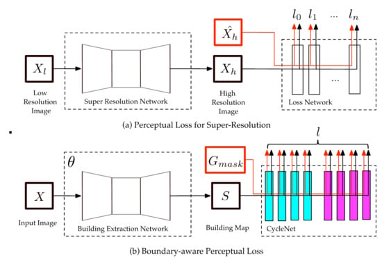
Apparently, CE loss just consider the similarities of and , and not explicitly capture the structural differences between the prediction and its corresponding ground truth. For example, consider two highly similar building maps where one has sharp corners and the other map has curved corners; despite their per-pixel similarity, they would be very different as measured by the difference in structural information. The basic idea of perceptual loss is that the structural information can be generated from high-level image feature representations extracted from pretrained CNN models. As shown in Figure 1a, a perceptual loss for super-resolution involves a feed-forward loss network pretrained on the image classification task and transfer loss functions to measure the difference in content between images. Hence, the usage of perceptual loss includes two stages. In the training stage, the loss network is trained to learn the structural information, and the learned structural information is embedded in the task-specific network via the transfer loss functions in the refining stage.
In the perceptual loss, the information learned by the loss network depends on which task it is trained for. The information learned from the image classification task is beneficial for super-resolution tasks, but it does not work on building extraction tasks. Rather than information learned from the image classification task, the structural information learned from the boundary extraction task has been proven to be effective in improving the accuracy of boundary areas on semantic segmentation [30]. However, the SEMEDA loss proposed in [30] is time-consuming since it has to jointly work with per-pixel cross-entropy loss to maintain the balance between extracting the structural information and the semantic information. Additionally, the performance of SEMEDA loss heavily relies on the hyper-parameter initializations. To overcome the problems above, the structural information and the semantic information are extracted simultaneously through one loss network in the proposed BP loss. The loss network is pretrained on a cyclical task: mask→boundary→mask; therefore, the loss network is named CycleNet. Additionally, a series of transfer loss functions is designed in the BP loss to measure the imbalance of positive samples in the building mask and boundary mask, the overview of the proposed BP loss is shown in Figure 1b. The architecture of CycleNet and its training schedules are described in Section 2.2. The schedules for applying the BP loss for boundary enhancements are introduced in Section 2.3.
2.2. CycleNet Architecture
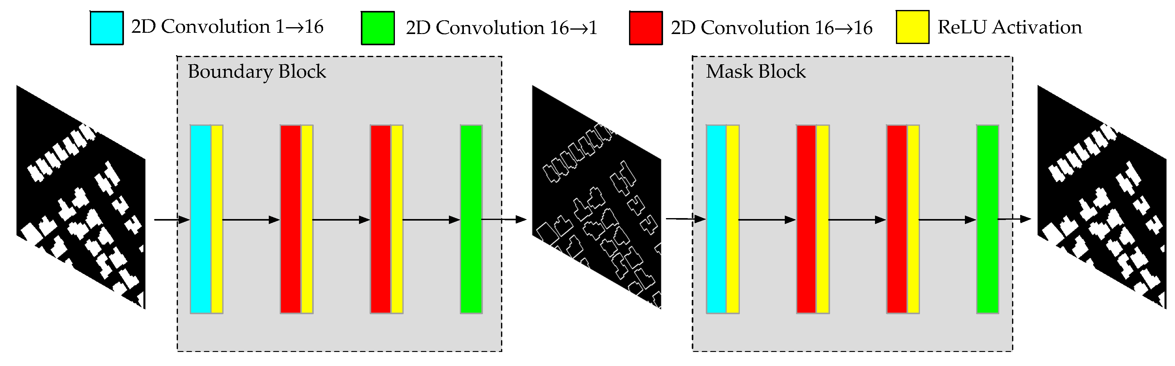
In this section, we describe the architecture of the proposed loss network: CycleNet and the schedule to train it. For further convenient analysis, we define the necessary symbolic representations in priority. is the VHR remote sensing image, which is the input of a building extraction network . The input of CycleNet is a building probability map predicted by , where ,, and indicate the channel, weight and height of the probability map, respectively. The weights of and are and , respectively. and are the building ground truth and its corresponding boundaries. Figure 2 shows the architecture of CycleNet. As shown in Figure 2, the architecture of CycleNet is quite simple and is cascaded with two identical blocks: boundary block and mask block . Each block has four 3 × 3 convolutional layers with ReLU activation layers sequentially, and the channels of the feature maps extracted in every layer are 16, 16, 16, and 1. The outputs of the mask block and boundary block are supervised with the building map and boundary map individually.
Unlike most of the perceptual loss approaches, we design a simple and shadow CNN model as the loss network to learn the structural information rather than directly applying existing pretrained backbone networks such as VGG-16 [29]. This is because learning the structural information from a binary building map is much easier than learning the colorful image. In CycleNet, the structural information is learned in boundary block by extracting the boundary map from the building map. However, similar to the CRF-based method [25], embedding only the structural information loses the semantic information. Thus, we design a symmetric mask block to maintain the semantic information of the input building map. It should be mentioned that a network with four convolutional layers cannot properly learn to generate the building map from a boundary map due to the limitation of its receptive field. Linking the mask block at the tail of the boundary block can ensure that the semantic information from the input building map is properly retained and transferred. A simple schedule is proposed to train CycleNet: the ground truth of the building map and its corresponding boundary map are utilized to jointly supervise the outputs of the last layers of the boundary block and the mask block, respectively. The loss function here is the classical loss, which is shown in Equation (2):
The definitions of are the same as those in Equation (1). Compared with the widely used cross-entropy loss, L1 loss is more sensitive to the variation in the local information, which is critical to learning the structural information. The softmax layer and batch norm layer are not involved in the CycleNet since these operations would restrict the scale of feature values. For the same reason, the ReLU function is chosen as the activation function. The training procedure of the proposed CycleNet can be simply formed as Equation (3):
Training CycleNet is called the training stage of the proposed BP loss, which is specified in Algorithm 1.
| Algorithm 1 Training the CycleNet |
| Training Model: CycleNe Input: Ground Truth Building Mask Ground Truth Building Boundary Output: Parameter of CycleNet for epoch in Total Epoch: End for |
2.3. Transfer Loss Functions
In this section, we introduce the schedule of the refining stage by applying the proposed transfer loss functions to enhance the building extraction performance with the structural information learned in CycleNet. In this stage, the CycleNet in the proposed BP loss is just a feed-forward network, and the parameter of CycleNet is fixed. Similar to the refining stage of the classical perceptual loss, the ground truth and the predicted building map from the building extraction network are separately fed into the pretrained CycleNet . With the input of , the extracted features from the nth convolutional layer in both the boundary block and mask block are represented by , (, ), respectively, and . The transfer loss functions are used to minimize the error between , and , . In most perceptual loss methods, naive per-pixel loss functions such as cross-entropy loss or are applied as transfer loss functions. However, with naive per-pixel loss, the unbalance phenomenon of positive pixel samples in the building map and the boundary map results in the situation that the structural information extracted from the boundary block cannot be efficiently embedded into the pipeline network, which causes the CycleNet to regress into the mask block only. Therefore, we design the weighted loss as a transfer loss function to balance the structural information and semantic information from each block of the proposed CycleNet. Assuming that the number of positive pixels in a building map and that of its corresponding boundary map are and , respectively, the balanced weight is , and the transfer loss functions in the BP loss can be formed as Equations (4)–(7):
With the proposed transfer loss functions, the structural information can be easily embedded in the pipeline network without semantic information loss. This procedure can be simply formed as Equation (8):
The schedule of the refining stage is specified as Algorithm 2.
| Algorithm 2 Structural Information Embedding |
| Training Model: Pipeline Network Input: VHR Remote Sensing Image Ground Truth Building Mask Ground Truth Building Boundary Output: Parameter of Pipeline Network for epoch in Total Epoch: Generate the balance weight: End for |
In summary, the proposed BP loss consists of a loss network CycleNet and transfer loss functions. CycleNet is trained to learn the structural information in the training stage through Algorithm 1. In the refining stage, the structural information is embedded into the building extraction network through Algorithm 2.
3. Experiments and Analysis
In this section, we conduct ablation experiments to demonstrate how the proposed BP loss learns and embeds the structural information into building extraction networks. Within two representative building extraction models, we compare the performances of the proposed BP loss with some other popular loss functions. Additionally, we also evaluate the time cost to demonstrate the efficiency of BP loss. Finally, we compare the UNet and PSPNet refined with the proposed BP loss with some recent state-of-the-art (SOTA) building extraction models and report new SOTA results on two popular building extraction datasets. All experiments are developed on NVIDIA GTX-Titan GPUs with 12 GB memories.
3.1. Study Materials
In this section, we detail the study materials of this paper in priority, which includes datasets, boundary generated method and evaluation metrics.
3.1.1. Datasets
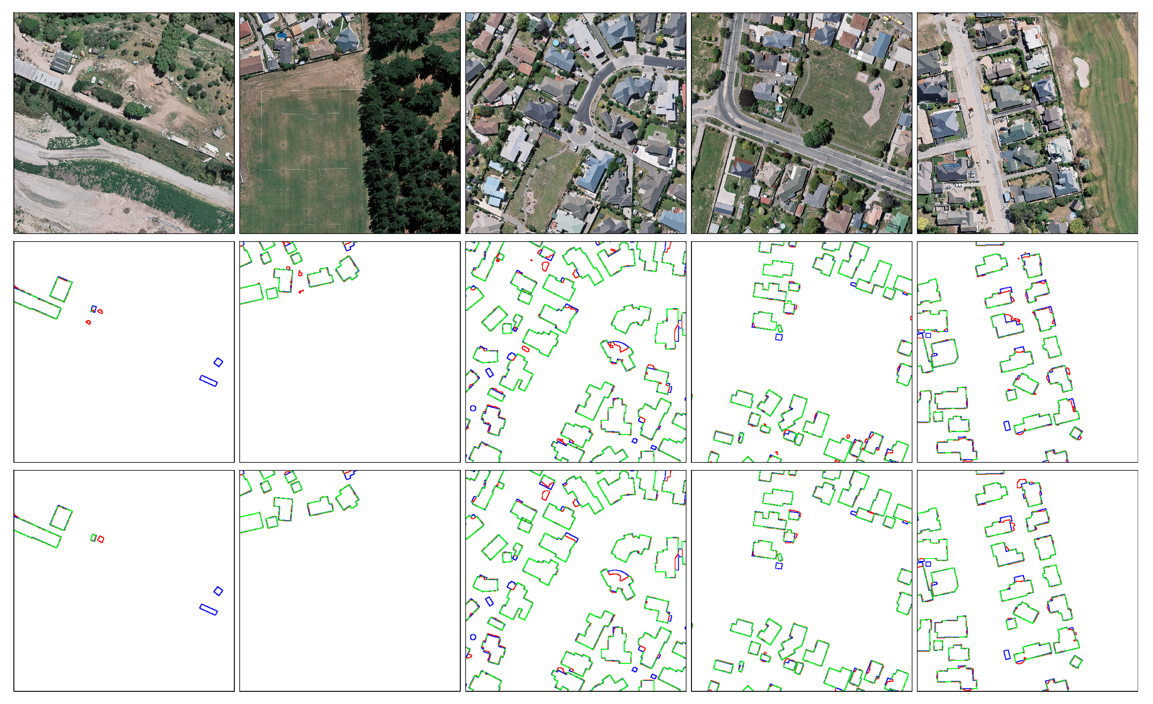
We conduct our experimental evaluations on two widely used and challenging datasets: the WHU aerial dataset [31] and the INRIA image labelling dataset [32]. The WHU aerial dataset includes 8,189 RGB tiles sized 512 × 512 from New Zealand, and more than 187,000 buildings are well labelled in this dataset. This dataset is officially divided into the training set, the validation set, and the testing set, which consists of 4736 images, 1036 images, and 2416 images, respectively. The spatial resolution of images in the WHU aerial dataset is 0.3 m (sampled from 0.075 m), and the whole dataset covers an area of approximately 450 . There are over 220,000 buildings extracted from New Zealand and all building labels in the WHU aerial dataset are generated by both the vector and raster maps and are artificially aligned. Thus, these high-quality labels are reliable and suitable for evaluating the performance of the proposed method. Another applied dataset is the INRIA image labelling dataset. Like the WHU dataset, the INRIA dataset has the same spatial resolution of 0.3 m. This dataset is collected from five different cities, including Austin, Chicago, Kitsap County, Vienna, and West Tyrol. There are 36 ortho-rectified 5000 × 5000 images covering for each region. Additionally, the five areas cover abundant landscapes ranging from highly dense metropolitan financial districts to alpine resorts. Following the official suggestions [32], we use 30 images (5th–36th) in every city for training and the others for testing. Images in the INRIA dataset are seamlessly cropped into 18,000 500 × 500 tiles. The landscapes and building styles of the INRIA dataset are much more complicated than those of the WHU dataset, and some of the labels are misaligned with the true buildings. The INRIA dataset is suitable for testing the robustness and generalization of the proposed method. Some samples of these two datasets are listed in Figure 3.
3.1.2. Boundary Generation
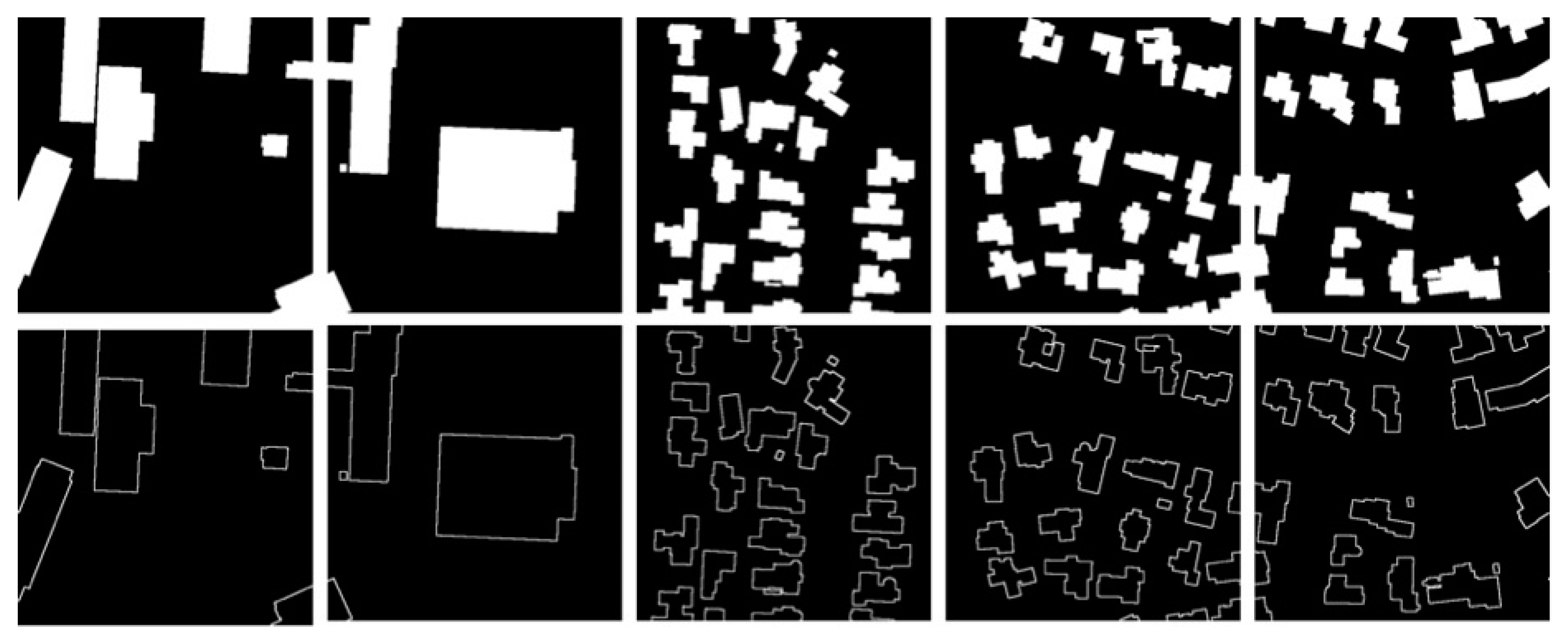
As described above, the boundary maps of buildings are required as extra labels to supervise CycleNet to learn the structural information in the training stage. The boundary ground truth is generated through a very simple method from the building ground truth, which is shown below. We first generate the all-zero with the same size as the building mask map . Then, for every pixel in , if it does not have the same value as its 2-neighbourhood (Manhattan distance) pixels, the pixel in the boundary map is assigned to be 1. After every pixel in is traversed, the boundary maps are generated. The pseudocode is illustrated in Algorithm 3.
| Algorithm 3 Boundary Generation |
| Input: Ground Truth Building Mask Output: Ground Truth Building Boundary Define for in : if any End for |
Some generated boundary maps are shown in Figure 4.
3.1.3. Evaluation Metrics
Following the official suggestions of the WHU aerial dataset [31] and the INRIA dataset [32], and with standard practices, overall accuracy, precision, recall, IoU and F1 score are used as the metrics to evaluate the performance of building extraction. However, for a boundary map, these per-pixel metrics cannot measure how close the predicted boundary is to its corresponding ground truth. Hence, we propose the structural accuracy (SA) score to evaluate the structural accuracy of the boundary areas of the predicted building map. First, we generate a copy of and name it . The pixel values on are assigned based on how close it is to the boundary pixels in . Pixels with 0, 1 and 2 distances are assigned 1, 0.5 and 0.25, respectively. Finally, we can obtain the SA index through Equation (9):
where is the boundary of the predicted building mask map, is the number of boundary pixels in , and denotes the dot product. For time efficiency, the bonus map and boundary map can be generated simultaneously within one traversal on , and a sample of a bonus map is shown in Figure 5.
3.2. Ablation Evaluation
In this section, we illustrate the results of learning the structural information in the training stage and embedding them into a building extraction network in the refining stage. For convenient comparison and analysis, we build all ablation experiments on the WHU aerial dataset. The results of the ablation experiments are evaluated only on overall accuracy and IoU metrics. Within the ablation experiments, we not only optimize the architecture of CycleNet to balance the memory/time cost and the building extraction performance but also test the adaptation of the proposed BP loss with other performance-enhanced loss functions.
3.2.1. Structural Information Embedding of the Boundary-Aware Perceptual Loss
In this section, we evaluate the architectures of CycleNet both in the training stage and the refining stage. In the training stage, the structural information (maskboundary) and the semantic information (boundary) embedding are simultaneously learned within the boundary block (BB) and the mask block (MB) of CycleNet. As shown in Table 1, we train CycleNet with different activation functions and loss functions for network architecture optimization. For comparison, we also train and test the BB and MB separately. The learning rate is fixed to 0.001, and the total epoch is 3.
From Table 1, on the one hand, both the boundary block and the CycleNet can properly extract the boundary map from the mask map because the maskboundary task can be performed with only local differential operations such as the Sobel operator [33], which can be easily simulated by CNN models within a limited number of convolutional layers. On the other hand, the mask block cannot transfer the boundary map into the mask map due to the limitation of the receptive field. However, CycleNet performs well on the boundarymask task because it maintains the semantic information from the input building map. The CycleNet with sigmoid activation function performs worse on both the maskboundary task and the maskboundary task than that with ReLU activation functions. With the ReLU function, the CycleNet trained with BCE loss (L1 loss) can achieve perfect IoU scores, which are 99.83% (99.56%) on the maskboundary task and 99.72% (99.58%) on the boundarymask task. This demonstrates that CycleNet with ReLU activation successfully learns the structural information embeddings. Regarding the choice of the loss function, BCE loss and L1 loss both work well; therefore, we evaluate the parameter weight distributions of the CycleNets trained with these 2 loss functions for further optimization, and the results are illustrated in Figure 6.
In Figure 6, we can see that the parameter weight distribution of the CycleNet trained with L1 loss is much sparser and tighter than that of BCE loss, which is critical for embedding the structural information into the building extraction network in the refining stage. With the abovementioned analysis, the CycleNet architecture with the ReLU activation function and L1 loss both properly learns the structural information and the semantic information and hence is chosen to build and train the CycleNet in the training stage.
Next, we conduct a series of ablation experiments on the refining stage to investigate how the BP loss with different architectures of CycleNet affects the performance improvements of building extraction networks on boundary areas. We apply the popular UNet [16] with the ResNet [34] backbone as the pipeline network to perform building extraction. Similar to most of the SOTA methods, we train the pipeline network following the schedule below: the learning rate is initialized to 0.001, and the pipeline network is trained for 60 epochs with binary cross-entropy (BCE) loss. For memory efficiency, we set the input batch size to 4, and the popular poly learning rate schedule, as shown in Equation (10), is also applied to adjust the learning weight.
where and represent the current and total epoch, respectively, and is set to 0.95 in our experiments. The pipeline network UNet-Res34 reaches 88.94% and 98.71% on IoU and Acc. Then, we refine the UNet-Res34 with the proposed BP loss of 4 alternative architecture designs of CycleNet. These CycleNet architectures are represented by the channels of the output in every convolutional layer of the boundary block (mask block), which are (16, 16, 1), (16, 32, 1), (16, 16, 16, 16, 1) and (16, 32, 16, 1). The naive L1 loss is also directly applied to refine the pipeline network as an extra control group. The epoch of the refining stage is 30, and the learning rate is set to 0.0001. The other hyperparameters are set with the same initializations as that of training the pipeline network. The quantity results are illustrated in Table 2.
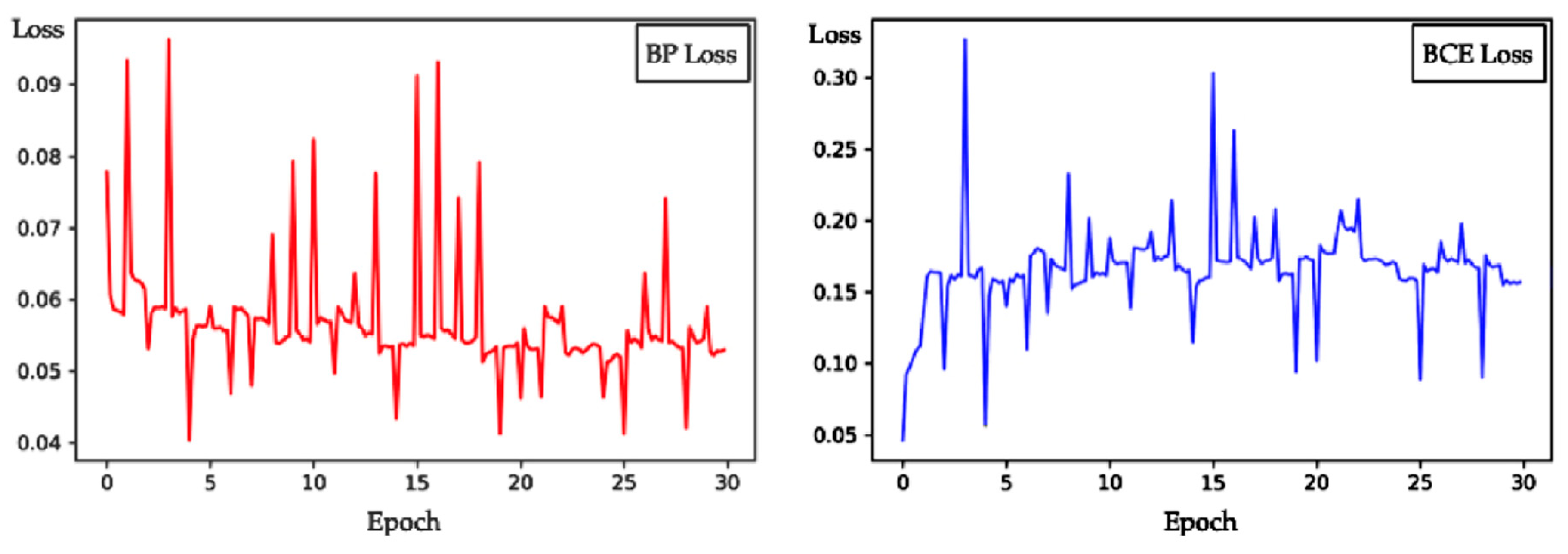
Apparently, the BP loss with 4 different CycleNet architectures improves the performance of the pipeline network both on overall accuracy and IoU scores. The simplest architecture (16, 16, 1) can significantly improve the IoU by 0.83%. The CycleNet of architecture (16, 32, 1) can obtain an IoU score of 89.81%. When we deepen these two blocks of CycleNet into 4 layers, the IoU of the (16, 16, 16, 1) architecture is increased to 90.11%. Moreover, the heavier CycleNet with the architecture of (16, 32, 16, 1) reaches the best performance of 90.27% on the IoU score, which is 1.33% higher than that of the naive pipeline network. Nevertheless, an inconspicuous IoU decrease in 0.14% is observed from the UNet refined with L1 loss. Based on the experimental results, the effectiveness of the proposed BP loss can be verified. The time efficiencies are also shown in Table 2. The refining stage of the BP loss requires an extra 12–25% training time, which is reasonable and acceptable for performance improvements. Finally, we select the architecture (16, 16, 16, 1) as the design of the CycleNet for the trade-off of effectiveness and efficiency. In Figure 7, we draw BP loss-epoch and BCE loss-epoch curves during refining the pipeline network to address the procedure of how the proposed BP loss embeds the structural information.
The sharp peaks periodically appear in these two curves, which are caused by the numerical instability at the start of every epoch. It can be seen from Figure 7 that the BP loss gradually decreases during the refining stage, while the BCE loss dramatically increases during the first several epochs. After that, the curve of BP loss fluctuates between 0.05 and 0.06, and BCE loss becomes stable near 0.15. This phenomenon indicates that the structural information embeddings break the balance of semantic information at the very beginning of the refining stage, and the balance of structural information and semantic information is reconstructed in a short time.
3.2.2. Adaptation of Boundary-aware Perceptual Loss
In this section, we evaluate the adaptative ability of the proposed BP loss with other SOTA performance-enhanced loss functions, including Jaccard loss, Dice loss, and trainable SEMEDA loss [30]. Similar to Section 3.2.1, UNet is selected as the pipeline building extraction network. The pipeline network is trained with these performance-enhanced loss functions in priority. Then, these trained pipeline networks are refined with the proposed BP loss for comparisons. The results are shown in Table 3.
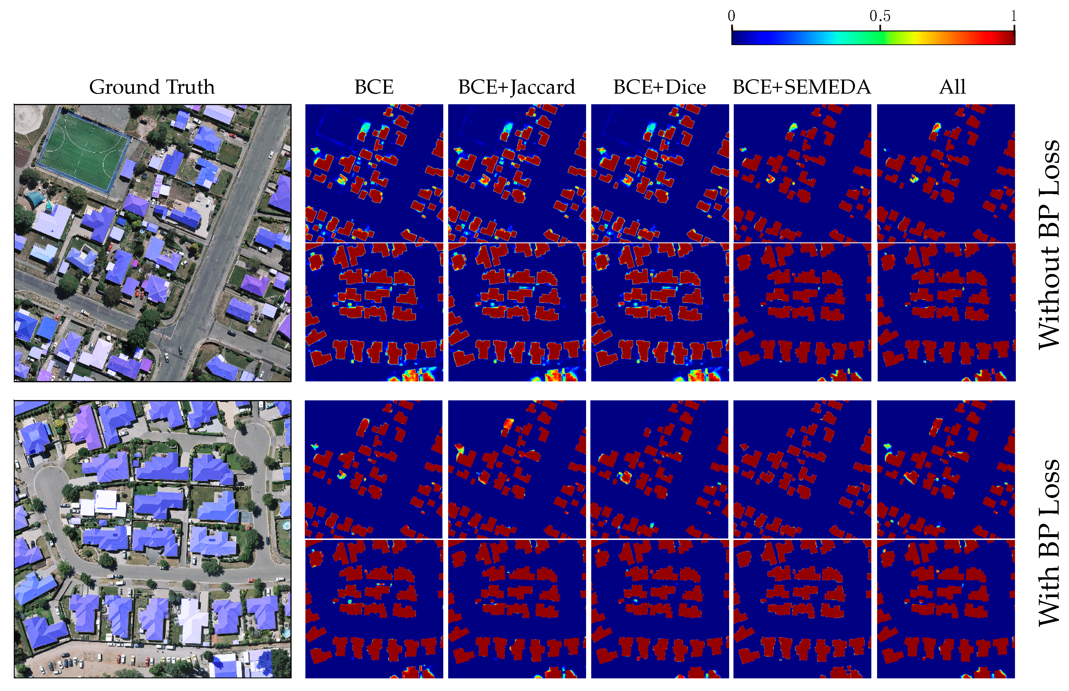
From Table 3, we can see that training the UNet with additional loss functions such as Jaccard loss, Dice loss and SEMEDA loss can obtain better performances. Compared with the untrainable loss functions such as Jaccard loss and Dice loss, the trainable SEMEDA loss effectively improves the IoU from 88.94% to 89.29%, while the Jaccard loss and the Dice loss only gain 0.17% and 0.24% IoU improvements, respectively. After the refinement of BP loss, the results of pipeline networks achieve further performance improvements. The IoU scores of UNet trained with BCE loss+Jaccard loss and BCE loss+Dice loss reach 90.11% and 90.21%, respectively. Nevertheless, only 0.62% of IoU improvements are observed from the UNet trained with SEMEDA loss, which is notably lower than the others. We think this is because the structural information learning with the loss networks of SEMEDA loss and BP loss overlaps. The inference time and space costs of the pipeline networks refined with either SEMEDA loss or the proposed BP loss are unchanged, while there are 15–20% extra time and memory costs during training and refining the pipeline networks. For comparisons, we visualize some predicted building probability maps from the pipeline networks before and after the refinement of the proposed BP loss in Figure 8.
Apparently, after the refinement of BP loss, the pixel values on the boundary area of buildings are much higher rather than the predictions from the naive pipeline networks, which means the network trained with BP loss is more confident for classifying the building boundary areas. Additionally, the unreliable predictions of the naive pipeline networks, where the activation is near 0.5, are activated better after the refinement with BP loss rather than that of SEMEDA loss.
3.3. Boundary Analyse
In this section, with the proposed BP loss, we evaluate how the structural information embedding affects the performance of building extraction on boundary areas with the metrics of accuracy, IoU, and SA score. The boundary map is generated from the prediction of the UNet pipeline network through Algorithm 3. The performances of the boundary maps before and after the refinement of the proposed BP loss are listed in Table 4.
Due to the phenomenon of uneven positive and negative pixels in the boundary map, the overall accuracies of the naive UNet and the refined UNet are both higher than 98%. Nonetheless, the boundary accuracy of the UNet +BP loss is still 0.15% higher than that of the naive UNet. The UNet+BP loss achieves 56.84% on IoU metrics, which is 3.29% higher than the naive UNet, which demonstrates that every pixel on the boundary areas achieves ‘absolutely’ more accurately. Additionally, refining the UNet with the proposed BP loss can increase the SA score by 1.44%, which means that the BP loss effectively makes the boundaries of predicted buildings much ‘closer’ to the ground truth. We list examples of the boundaries of the building maps predicted by the naive UNet and the refined UNet in Figure 9.
In Figure 9, we can see that after the refinement of the proposed BP loss, the boundary areas of the predicted building maps become much closer to the ground truth. Moreover, the boundaries of the predicted buildings become highly structural and regular without apparent semantic information loss. Additionally, some misclassification boundary areas existing in the predictions of the naive UNet are rectified through the BP loss refinement. These improvements can prove the effectiveness of the proposed BP loss.
3.4. SOTA Comparison
In this section, we apply the proposed BP loss on UNet and PSPNet and compare the results with very recent SOTA models both on the WHU dataset and the INRIA dataset. UNet uses symmetric jump connections to enhance the local information, while PSPNet applies a group of dilated convolutions to enrich the receptive fields and gain better semantic information. These two models are representative and typical in the pixel-wise labelling task; hence, refining with them can prove the reliabilities of the BP loss on most of the CNN models. The 101-layer ResNet is applied as the backbone of UNet and PSPNet due to its excellent feature extraction ability. To obtain highly reliable results, we train and refine the UNet and PSPNet for 60 epochs. The other experimental details are the same as those mentioned in Section 3.2.1. The results are listed in Table 5.
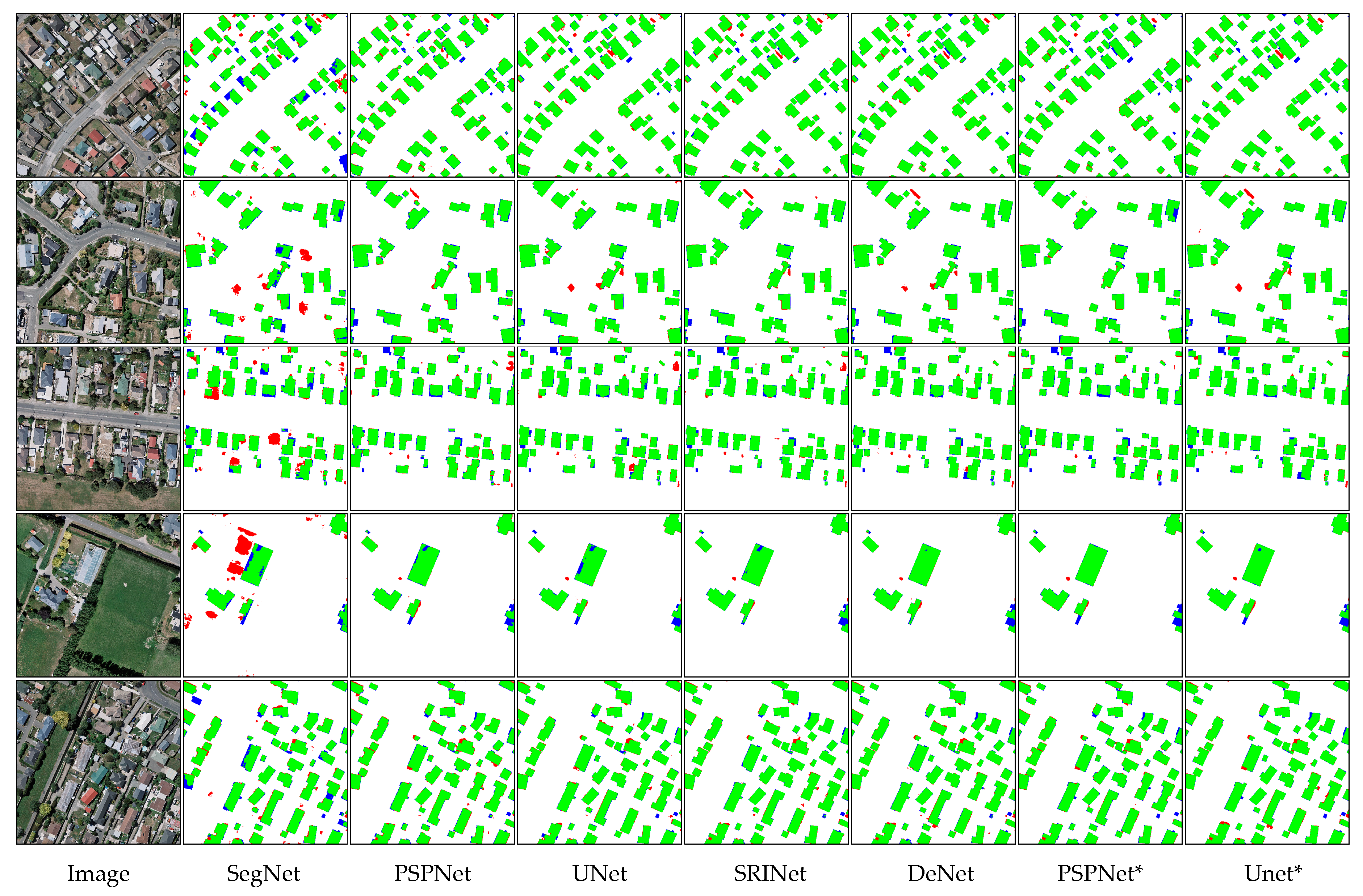
In Table 5, the performances of the naive PSPNet and the naive UNet are approximately 2% higher than SegNet on the IoU score, which proves the effectiveness of these two representative CNN architectures. Some very recent SOTA boundary-aware methods with carefully designed CNN architectures for building extraction tasks from VHR images, such as SiU-Net, SRINet, and DeNet, obtain much higher IoU scores, which are 88.40%, 89.04%, and 90.12%, respectively. Refined with the proposed BP loss, the performance of the naive PSPNet increases and reaches 88.78% on the IoU score. Moreover, the performance of UNet refined with BP loss increases to 90.78% on the IoU score, which is 0.66% higher than DeNet and achieves a new SOTA result. It is worth mentioning that the precision of methods applying dilated convolution, such as PSPNet and SRINet (94.42% and 95.31%), are generally higher than those of methods applying jump connections, such as UNet and SiU-Net (93.85% and 93.80%), while the methods applying jump connection architectures can achieve higher recall scores. With the proposed BP loss, these two kinds of models can be improved and obtain higher performances on every metric score. Some randomly selected samples are shown in Figure 10 for visual comparison.
With the same hyper-parameter initializations, the experimental results on the INRIA dataset are shown in Table 6.
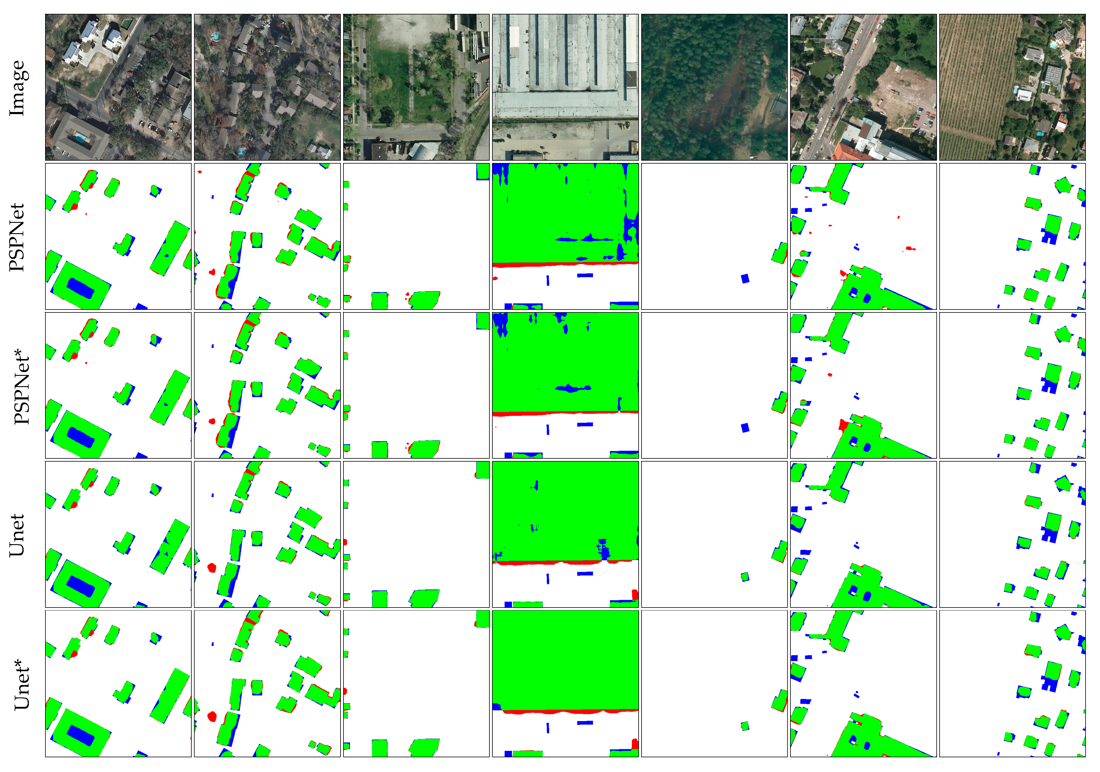
Following the official suggestions in [32], we only use overall accuracy and IoU to evaluate the results over five different areas in the INRIA dataset. From Table 6, we can see that every model does not perform as well as that on the WHU aerial dataset due to the complexity and difficulty of the INRIA dataset. Very naive SegNet only achieves 70.81% IoU. There is an approximately 3% IoU improvement after applying a multi-task loss on SegNet with an extra distance map. Among these methods, the RiFCN, which applied another RNN to align the feature maps extracted from the FCN model, and achieves the SOTA result, which is 74.00% on the IoU score. Benefitting from the perfect quality of the open-source semantic segmentation project on https://github.com/qubvel/segmentation_models.pytorch, the pipeline networks PSPNet and UNet achieve comparable results of 73.99% and 75.78% IoU scores, respectively. Refined with the proposed BP loss, the performance of PSPNet increased by 1.69% on the IoU score, while 1.04% of IoU improvements are also observed on UNet. In detail, the performances of different models fluctuate over the five areas. The IoU scores of models on Austin and Vienna are distinctively higher than those of the remaining three areas. Some images and the corresponding building maps extracted with different models are visualized in Figure 11.
In Figure 11, we find that the performance of the models is visually less acceptable than that of the WHU aerial dataset, especially on unregular building areas or areas where the buildings are covered by vegetation. Nevertheless, the models refined with the proposed BP loss can gain significant performance improvements on the boundary areas of both large-scale and small-scale buildings. For small-scale buildings, most of the drop-like false-positive predictions are removed due to the embedding of the structural information. For large-scale buildings, the consistency of building boundaries is tremendously increased after structural information embedding.
4. Conclusions
In this paper, we proposed an improved boundary-aware perceptual loss to enhance the performance of building extraction networks on boundary areas. The proposed BP loss involves a carefully designed loss network named CycleNet aiming at learning the structural information and a series of transfer loss functions aiming at transferring the learned structural information. The experimental results on the WHU dataset and the INRIA aerial image labelling dataset demonstrated the effectiveness, efficiency and robustness of the proposed BP loss. Rather than the networks specifically designed and optimized for the building extraction task, the proposed BP loss has better adaptivity, and fewer knowledge and hardware requirements. Nevertheless, the proposed BP loss does not work as well on uncommon-scale buildings with irregular shapes or areas covered by shadows or vegetation. For this purpose, embedding the morphology information into a building extraction network will be the focus of our future work.
Author Contributions
The work presented in this paper was developed collaboratively by all the authors. Y.Z. proposed the whole segmentation framework and designed and conducted the experiments; W.L. is the corresponding author of this research work; W.G. was involved in the writing and argumentation of the manuscript; Z.W. and J.S. were involved in experimental analysis. All authors have read and agreed to the published version of the manuscript.
Funding
This work was funded by the Key Projects of Science and Technology Agency of Guangxi province, China (Guike AA 17129002); National Science and Technology Key Program of China (2013GS500303); and the Municipal Science and Technology Project of CQMMC, China (2017030502).
Acknowledgments
We thank Inria for providing the Inria Aerial Image Labelling Dataset and the WHU Aerial Dataset on their website (https://project.inria.fr/aerialimagelabelling/, http://study.rsgis.whu.edu.cn/pages/download/). We are also very grateful for the valuable suggestions and comments of peer reviewers.
Conflicts of Interest
The authors declare no conflict of interest.
References
- Huang, H.; Xu, K. Combing Triple-Part Features of Convolutional Neural Networks for Scene Classification in Remote Sensing. Remote. Sens. 2019, 11, 1687. [Google Scholar] [CrossRef] [Green Version]
- Zhu, R.; Yan, L.; Mo, N.; Liu, Y. AttentionBased Deep Feature Fusion for the Scene Classification of HighResolution Remote Sensing Images. Remote. Sens. 2020, 12, 742. [Google Scholar] [CrossRef] [Green Version]
- Cui, B.; Zhang, Y.; Yan, L.; Wei, J.; Wu, H. An Unsupervised SAR Change Detection Method Based on Stochastic Subspace Ensemble Learning. Remote. Sens. 2019, 11, 1314. [Google Scholar] [CrossRef] [Green Version]
- Li, L.; Wang, C.; Zhang, H.; Zhang, B.; Wu, F. Urban Building Change Detection in SAR Images Using Combined Differential Image and Residual U-Net Network. Remote. Sens. 2019, 11, 1091. [Google Scholar] [CrossRef] [Green Version]
- Mahdavi, S.; Salehi, B.; Huang, W.; Amani, M.; Brisco, B. A PolSAR Change Detection Index Based on Neighborhood Information for Flood Mapping. Remote. Sens. 2019, 11, 1854. [Google Scholar] [CrossRef] [Green Version]
- Chen, C.; Gong, W.; Chen, Y.; Li, W. Object Detection in Remote Sensing Images Based on a Scene-Contextual Feature Pyramid Network. Remote. Sens. 2019, 11, 339. [Google Scholar] [CrossRef] [Green Version]
- Pan, X.; Yang, F.; Gao, L.; Chen, Z.; Zhang, B.; Fan, H.; Ren, J. Building Extraction from High-Resolution Aerial Imagery Using a Generative Adversarial Network with Spatial and Channel Attention Mechanisms. Remote Sens. 2019, 11, 917. [Google Scholar] [CrossRef] [Green Version]
- Zhang, Y.; Gong, W.; Sun, J.; Li, W. Web-Net: A Novel Nest Networks with Ultra-Hierarchical Sampling for Building Extraction from Aerial Imageries. Remote. Sens. 2019, 11, 1897. [Google Scholar] [CrossRef] [Green Version]
- Neuville, R.; Pouliot, J.; Poux, F.; Billen, R. 3D Viewpoint Management and Navigation in Urban Planning: Application to the Exploratory Phase. Remote. Sens. 2019, 11, 236. [Google Scholar] [CrossRef] [Green Version]
- Khanal, N.; Uddin, K.; Matin, M.; Tenneson, K. Automatic Detection of Spatiotemporal Urban Expansion Patterns by Fusing OSM and Landsat Data in Kathmandu. Remote. Sens. 2019, 11, 2296. [Google Scholar] [CrossRef] [Green Version]
- Long, J.; Shelhamer, E.; Darrell, T. Fully Convolutional Networks for Semantic Segmentation. In Proceedings of the 2015 Ieee Conference on Computer Vision and Pattern Recognition, Boston, MA, USA, 7–12 June 2015; pp. 3431–3440. [Google Scholar]
- Ibtehaz, N.; Rahman, M.S. MultiResUNet : Rethinking the U-Net architecture for multimodal biomedical image segmentation. Neural Netw. 2020, 121, 74–87. [Google Scholar] [CrossRef]
- Zhao, J.; He, X.; Li, J.; Feng, T.; Ye, C.; Xiong, L. Automatic Vector-Based Road Structure Mapping Using Multibeam LiDAR. Remote. Sens. 2019, 11, 1726. [Google Scholar] [CrossRef] [Green Version]
- Huang, J.; Zhang, X.; Xin, Q.; Sun, Y.; Zhang, P. Automatic building extraction from high-resolution aerial images and LiDAR data using gated residual refinement network. ISPRS J. Photogramm. Remote. Sens. 2019, 151, 91–105. [Google Scholar] [CrossRef]
- Sun, G.; Huang, H.; Zhang, A.; Li, F.; Zhao, H.; Fu, H. Fusion of Multiscale Convolutional Neural Networks for Building Extraction in Very High-Resolution Images. Remote. Sens. 2019, 11, 227. [Google Scholar] [CrossRef] [Green Version]
- Ronneberger, O.; Fischer, P.; Brox, T. U-Net: Convolutional Networks for Biomedical Image Segmentation. In Medical Image Computing and Computer-Assisted Intervention, Pt Iii; Navab, N., Hornegger, J., Wells, W.M., Frangi, A.F., Eds.; Springer: Cham, Switzerland, 2015; Volume 9351, pp. 234–241. [Google Scholar]
- Peng, D.; Zhang, Y.; Guan, H. Guan End-to-End Change Detection for High Resolution Satellite Images Using Improved UNet++. Remote. Sens. 2019, 11, 1382. [Google Scholar] [CrossRef] [Green Version]
- Yue, K.; Yang, L.; Li, R.; Hu, W.; Zhang, F.; Li, W. TreeUNet: Adaptive Tree convolutional neural networks for subdecimeter aerial image segmentation. ISPRS J. Photogramm. Remote. Sens. 2019, 156, 1–13. [Google Scholar] [CrossRef]
- Badrinarayanan, V.; Badrinarayanan, V.; Cipolla, R. SegNet: A Deep Convolutional Encoder-Decoder Architecture for Image Segmentation. IEEE Trans. Pattern Anal. Mach. Intell. 2017, 39, 2481–2495. [Google Scholar] [CrossRef] [PubMed]
- Zhou, Z.W.; Siddiquee, M.M.R.; Tajbakhsh, N.; Liang, J.M. UNet plus plus : A Nested U-Net Architecture for Medical Image Segmentation. In Deep Learning in Medical Image Analysis and Multimodal Learning for Clinical Decision Support, Dlmia 2018; Stoyanov, D., Taylor, Z., Carneiro, G., SyedaMahmood, T., Eds.; Springer: Cham, Switzerland, 2018; Volume 11045, pp. 3–11. [Google Scholar]
- Wu, G.; Shao, X.; Guo, Z.; Chen, Q.; Yuan, W.; Shi, X.; Xu, Y.; Shibasaki, R. Automatic Building Segmentation of Aerial Imagery Using Multi-Constraint Fully Convolutional Networks. Remote. Sens. 2018, 10, 407. [Google Scholar] [CrossRef] [Green Version]
- Zhao, H.; Shi, J.; Qi, X.; Wang, X.; Jia, J. Pyramid Scene Parsing Network. In Proceedings of the 30th Ieee Conference on Computer Vision and Pattern Recognition, Honolulu, HI, USA, 21–26 July 2017; pp. 6230–6239. [Google Scholar]
- Chen, L.C.; Zhu, Y.; Papandreou, G.; Schroff, F.; Adam, H. Encoder-Decoder with Atrous Separable Convolution for Semantic Image Segmentation. In Proceedings of the European Conference on Computer Vision (ECCV), Munich, Germany, 8–14 September 2018. [Google Scholar]
- Krähenbühl, P.; Koltun, V. Efficient Inference in Fully Connected CRFs with Gaussian Edge Potentials. Available online: http://papers.nips.cc/paper/4296-efficient-inference-in-fully-connected-crfs-with-gaussian-edge-potentials.pdf (accessed on 8 April 2020).
- Zheng, S.; Jayasumana, S.; Romera-Paredes, B.; Vineet, V.; Su, Z.; Du, D.; Huang, C.; Torr, P.H.S. Conditional Random Fields as Recurrent Neural Networks. In Proceedings of the 2015 Ieee International Conference on Computer Vision, Santiago, Chile, 7–13 December 2015; pp. 1529–1537. [Google Scholar]
- Bertels, J.; Eelbode, T.; Berman, M.; Vandermeulen, D.; Maes, F.; Bisschops, R.; Blaschko, M.B. Optimizing the Dice score and Jaccard index for medical image segmentation: Theory and practice. In International Conference on Medical Image Computing and Computer-Assisted Intervention; Springer: Cham, Switzerland, 2019; pp. 92–100. [Google Scholar]
- Iglovikov, V.; Shvets, A. TernausNet: U-Net with VGG11 Encoder Pre-Trained on ImageNet for Image Segmentation. arXiv 2018, arXiv:1801.05746. [Google Scholar]
- Johnson, J.; Alahi, A.; Li, F.-F. Perceptual Losses for Real-Time Style Transfer and Super-Resolution. In Computer Vision-Eccv 2016, Pt Ii; Leibe, B., Matas, J., Sebe, N., Welling, M., Eds.; Springer: Cham, Switzerland, 2016; Volume 9906, pp. 694–711. [Google Scholar]
- Simonyan, K.; Zisserman, A. Very deep convolutional networks for large-scale image recognition. arXiv 2014, arXiv:1409.1556. [Google Scholar]
- Chen, Y.; Dapogny, A.; Cord, M. SEMEDA: Enhancing Segmentation Precision with Semantic Edge Aware Loss. arXiv 2019, arXiv:1905.01892. [Google Scholar]
- Ji, S.; Wei, S.; Lu, M. Fully Convolutional Networks for Multisource Building Extraction From an Open Aerial and Satellite Imagery Data Set. IEEE Trans. Geosci. Remote. Sens. 2018, 57, 574–586. [Google Scholar] [CrossRef]
- Maggiori, E.; Tarabalka, Y.; Charpiat, G.; Alliez, P. Can semantic labeling methods generalize to any city? The inria aerial image labeling benchmark. In Proceedings of the 2017 IEEE International Geoscience and Remote Sensing Symposium (IGARSS), Worth, TX, USA, 23–28 July 2017; pp. 3226–3229. [Google Scholar]
- Sobel, I. History and Definition of the Sobel Operator. Retrieved from the World Wide Web 2014, 1505. Available online: https://www.researchgate.net/publication/239398674_An_Isotropic_3x3_Image_Gradient_Operator (accessed on 8 April 2020).
- He, K.; Zhang, X.; Ren, S.; Sun, J. Deep Residual Learning for Image Recognition. In Proceedings of the 2016 Ieee Conference on Computer Vision and Pattern Recognition, Las Vegas, NV, USA, 27–30 June 2016; pp. 770–778. [Google Scholar]
- Liu, P.; Liu, X.; Liu, M.; Shi, Q.; Yang, J.; Xu, X.; Zhang, Y. Building Footprint Extraction from High-Resolution Images via Spatial Residual Inception Convolutional Neural Network. Remote. Sens. 2019, 11, 830. [Google Scholar] [CrossRef] [Green Version]
- Liu, H.; Luo, J.; Huang, B.; Hu, X.; Sun, Y.; Yang, Y.; Xu, N.; Zhou, N. DE-Net: Deep Encoding Network for Building Extraction from High-Resolution Remote Sensing Imagery. Remote. Sens. 2019, 11, 2380. [Google Scholar] [CrossRef] [Green Version]
- Bischke, B.; Helber, P.; Folz, J.; Borth, D.; Dengel, A. Multi-task learning for segmentation of building footprints with deep neural networks. arXiv 2017, arXiv:1709.05932. [Google Scholar]
- Mou, L.; Zhu, X.X. RiFCN: Recurrent network in fully convolutional network for semantic segmentation of high resolution remote sensing images. arXiv 2018, arXiv:1805.02091. [Google Scholar]
Figure 1.
(a) and (b) are the overviews of the classical perceptual loss for the super-resolution task and the proposed boundary-aware perceptual (BP) loss for the building extraction task, respectively. In (a), and are the low-resolution input image and its corresponding high-resolution prediction, respectively, and is the ground truth of . is the transfer function of the nth layer. In (b), X is the input remote sensing image, and S and are the predicted building map and the ground truth of the building map, respectively. The light blue and violet cubes represent the boundary block and mask block in CycleNet. represents the transfer loss functions.

Figure 2.
Overview of the CycleNet architecture. The yellow rectangle represents the ReLU activation layer. The other three colors of rectangles dedicate 3 different convolutional layers, and the padding and stride are consistently set to 1. The kernel size of the convolution layer with the color of light blue, red and green are 1 × 16 × 3 × 3, 16 × 16 × 3 × 3 and 16 × 1 × 3 × 3, respectively. The boundary map is predicted from a building mask map through a boundary block, while the mask block map recovers the boundary map back into the building mask map.

Figure 3.
Visual close-ups of the WHU aerial dataset and the INRIA dataset. Images of the first (second) row are randomly selected from the training set of the WHU (INRIA) aerial dataset.
Figure 3.
Visual close-ups of the WHU aerial dataset and the INRIA dataset. Images of the first (second) row are randomly selected from the training set of the WHU (INRIA) aerial dataset.

Figure 4.
The boundary maps in the second row are generated from the building mask map in the first row through Algorithm 3.
Figure 4.
The boundary maps in the second row are generated from the building mask map in the first row through Algorithm 3.

Figure 5.
(a) is a cropped bin from the VHR image, (b) is the building mask map, (c) is the boundary mask and (d) is the generated bonus map where pixels of red, green, blue and black colors represent the values of 1, 0.5, 0.25 and 0, respectively.
Figure 5.
(a) is a cropped bin from the VHR image, (b) is the building mask map, (c) is the boundary mask and (d) is the generated bonus map where pixels of red, green, blue and black colors represent the values of 1, 0.5, 0.25 and 0, respectively.

Figure 6.
The parameter weight distribution of the CycleNets trained with L1 loss (left) and BCE loss (right).
Figure 6.
The parameter weight distribution of the CycleNets trained with L1 loss (left) and BCE loss (right).

Figure 7.
Diagram of the proposed BP loss and BCE loss during refining the naive UNet-Res34.

Figure 8.
The images and corresponding masks are listed in the first column. Starting with the second column, the top parts of the building probability maps are predicted from the pipeline networks trained with BCE loss, BCE+Jaccard loss, BCE+Dice loss, BCE+SEMEDA loss and with all 4 losses together. With the same order, the building probability maps predicted from the pipeline networks refined with BP loss are located on the bottom part.

Figure 9.
Examples of the building boundaries. The 2nd and 3rd are boundary maps predicted from images in the 1st row through the naive UNet and the UNet refined with the BP loss, respectively. Areas of green, red, blue, and white represent the true-positive, false-positive, false-negative and true-negative predictions, respectively.

Figure 10.
The building maps from the 2nd–6th columns are produced from the images in the 1st column using SegNet, PSPNet, UNet, SRINet, and DeNet. The predicted building maps of PSPNet and UNet refined with BP loss are located in the last 2 columns. * indicates that the model is refined with the proposed BP loss.

Figure 11.
Results on the different areas of the INRIA dataset. From the 2nd to the 5th, the building maps are predicted from the naive PSPNet, refined PSPNet, UNet, and refined UNet.
Figure 11.
Results on the different areas of the INRIA dataset. From the 2nd to the 5th, the building maps are predicted from the naive PSPNet, refined PSPNet, UNet, and refined UNet.


Table 1.
The IoU of boundary and mask from the test set of the WHU aerial dataset in the training stage.
Table 1.
The IoU of boundary and mask from the test set of the WHU aerial dataset in the training stage.
| Block | Boundary IoU (%) | Mask IoU (%) |
|---|---|---|
| Boundary Block (Sigmoid+BCE) | 97.94 | — |
| Boundary Block (Relu+BCE) | 99.96 | — |
| Boundary Block (Relu+L1) | 99.69 | — |
| Mask Block (Sigmoid+BCE) | — | 16.46 |
| Mask Block (Relu+BCE) | — | 12.77 |
| Mask Block (Relu+L1) | — | 9.83 |
| CycleNet (Sigmoid+BCE) | 96.64 | 98.10 |
| CycleNet (Relu+BCE) | 99.83 | 99.72 |
| CycleNet (Relu+L1) | 99.56 | 99.58 |
Table 2.
The intersection over union (IoU) of Res34-UNet with BP loss on the WHU dataset.
| Architecture | Acc (%) | Mask IoU (%) | Time (fps) |
|---|---|---|---|
| (16, 16, 1) | 98.80(+0.09) | 89.77(+0.83) | 2.04 |
| (16, 32, 1) | 98.81(+0.10) | 89.81(+0.87) | 1.95 |
| (16, 16, 16, 1) | BP 98.85(+0.14) | 90.11(+1.17) | 1.88 |
| (16, 32, 16, 1) | 98.86(+0.15) | 90.27(+1.33) | 1.71 |
| L1 Loss | 98.68(-0.03) | 88.57(-0.14) | 2.31 |
Table 3.
IoU on the WHU dataset with UNet-Res34 trained with various loss functions.
| UNet-Res34 | |||||
| BCE Loss | ✓ | ✓ | ✓ | ✓ | ✓ |
| Jaccard Loss | ✓ | ✓ | |||
| Dice Loss | ✓ | ✓ | |||
| SEMEDA Loss | ✓ | ✓ | |||
| Acc (%) IoU (%) | 98.71 | 98.73 | 98.74 | 98.75 | 98.77 |
| 88.94 | 89.11 | 89.18 | 89.29 | 89.37 | |
| UNet-Res34+BP Loss | |||||
| Acc (%) IoU (%) | 98.85 | 98.84 | 98.86 | 98.81 | 98.89 |
| 90.11 | 90.07 | 90.21 | 89.81 | 90.40 | |
Table 4.
Predicted boundary performance on the WHU dataset.
| UNet | UNet +BP Loss | |
|---|---|---|
| Acc (%) | 98.47 | 98.62 |
| IoU (%) | 53.55 | 56.84 |
| SA (%) | 78.42 | 79.86 |
Table 5.
SOTA comparisons on the WHU dataset.
| Method | Acc (%) | IoU (%) | Precision (%) | Recall (%) | F1(%) |
|---|---|---|---|---|---|
| SegNet [19] | - | 86.58 | 92.55 | 93.06 | 92.80 |
| PSPNet [22] | 98.61 | 88.14 | 94.42 | 92.99 | 93.70 |
| UNet [16] | 98.74 | 89.31 | 93.85 | 94.87 | 94.35 |
| SiU-Net [31] | - | 88.40 | 93.80 | 93.90 | - |
| SRINet [35] | - | 89.09 | 95.21 | 93.28 | 94.23 |
| DeNet [36] | 90.12 | 95.00 | 94.60 | 94.80 | |
| PSPNet+BP Loss | 98.69 | 88.78 | 95.02 | 93.14 | 94.07 |
| UNet+BP Loss | 98.84 | 90.78 | 95.06 | 94.89 | 94.97 |
Table 6.
SOTA comparisons on the INRIA dataset.
| Methods | Austin | Chicago | Kitsap Country | Western Tyrol | Vienna | Overall | |
|---|---|---|---|---|---|---|---|
| SegNet (Single-Loss) [37] | IoU | 74.81 | 52.83 | 68.06 | 65.68 | 72.90 | 70.14 |
| Acc. | 92.52 | 98.65 | 97.28 | 91.36 | 96.04 | 95.17 | |
| SegNet (Multi-Task Loss) [37] | IoU | 76.76 | 67.06 | 73.30 | 66.91 | 76.68 | 73.00 |
| Acc. | 93.21 | 99.25 | 97.84 | 91.71 | 96.61 | 95.73 | |
| RiFCN [38] | IoU | 76.84 | 67.45 | 63.95 | 73.19 | 79.18 | 74.00 |
| Acc. | 96.50 | 91.76 | 99.14 | 97.75 | 93.95 | 95.82 | |
| UNet [16] | IoU | 78.51 | 68.53 | 66.36 | 77.48 | 80.26 | 75.58 |
| Acc. | 97.05 | 92.69 | 99.29 | 98.30 | 94.56 | 96.38 | |
| PSPNet [22] | IoU | 75.05 | 69.93 | 61.09 | 73.32 | 78.06 | 73.99 |
| Acc. | 96.48 | 93.11 | 99.11 | 97.88 | 93.90 | 96.10 | |
| UNet+BP Loss | IoU | 79.59 | 70.06 | 68.04 | 78.97 | 80.84 | 76.62 |
| Acc. | 97.20 | 92.90 | 99.33 | 98.42 | 94.76 | 96.52 | |
| PSPNet+BP Loss | IoU | 76.80 | 71.51 | 62.51 | 73.90 | 80.17 | 75.68 |
| Acc. | 96.82 | 93.58 | 99.16 | 98.05 | 94.65 | 96.45 |
© 2020 by the authors. Licensee MDPI, Basel, Switzerland. This article is an open access article distributed under the terms and conditions of the Creative Commons Attribution (CC BY) license (http://creativecommons.org/licenses/by/4.0/).
Share and Cite
MDPI and ACS Style
Zhang, Y.; Li, W.; Gong, W.; Wang, Z.; Sun, J. An Improved Boundary-Aware Perceptual Loss for Building Extraction from VHR Images. Remote Sens. 2020, 12, 1195. https://doi.org/10.3390/rs12071195
AMA Style
Zhang Y, Li W, Gong W, Wang Z, Sun J. An Improved Boundary-Aware Perceptual Loss for Building Extraction from VHR Images. Remote Sensing. 2020; 12(7):1195. https://doi.org/10.3390/rs12071195
Chicago/Turabian StyleZhang, Yan, Weihong Li, Weiguo Gong, Zixu Wang, and Jingxi Sun. 2020. "An Improved Boundary-Aware Perceptual Loss for Building Extraction from VHR Images" Remote Sensing 12, no. 7: 1195. https://doi.org/10.3390/rs12071195
Note that from the first issue of 2016, this journal uses article numbers instead of page numbers. See further details here.