A line integral approach for the computation of the potential harmonic coefficients of a constant density polyhedron

Abstract

A novel approach for the computation of the spherical harmonic coefficients of the gravity field of a constant density polyhedron is presented. The proposed method is based on the expression of these coefficients as the volume integral of solid harmonics. It is well known that the divergence theorem leads to an expression of these volume integrals as surface integrals. We show that these surface integrals can be expressed as the sum of line integrals along the edges of the polyhedron. In contrast to previous approaches, the values of the spherical harmonic coefficients at a given degree and order result directly from the computation of the line integrals. The performed numerical implementation revealed the stability of the proposed algorithm up to degree 360 for a prismatic test source.

Appendix

1.1 A.1 Derivative of $h_{n,m}$ along the z-axis

The relation expressed by Eq. (7) is obtained in polar coordinates as follows (the calculus is identical with a $\sin \left( m\lambda \right)$ dependency to the longitude)

$$\begin{aligned}&\frac{\partial h_{n,m}^{c}\left( \rho ,\lambda ,z\right) }{\partial z} \\&\quad = \frac{\partial }{\partial z}\left( \left( \rho ^{2}+z^{2}\right) ^{\frac{n}{2}}P_{n,m}\left( \frac{z}{\sqrt{\rho ^{2}+z^{2}}}\right) \cos (m\lambda )\right) \\&\quad = \frac{\partial \left( \rho ^{2}+z^{2}\right) ^{\frac{n}{2}}}{\partial z}P_{n,m}\left( \frac{z}{\sqrt{\rho ^{2}+z^{2}}}\right) \cos (m\lambda ) \\&\qquad +\left( \rho ^{2}+z^{2}\right) ^{\frac{n}{2}}\frac{\partial }{\partial z}P_{n,m}\left( \frac{z}{\sqrt{\rho ^{2}+z^{2}}}\right) \cos (m\lambda ) \end{aligned}$$

We have

$$\begin{aligned} \frac{\partial \left( \rho ^{2}+z^{2}\right) ^{\frac{n}{2}}}{\partial z}=nz\left( \rho ^{2}+z^{2}\right) ^{\frac{n}{2}-1} \end{aligned}$$

and

$$\begin{aligned} \frac{\partial }{\partial z}P_{n,m}\left( \frac{z}{\sqrt{\rho ^{2}+z^{2}}}\right)= & {} \frac{1}{\sqrt{\rho ^{2}+z^{2}}}\left( 1-\left( \frac{z}{\sqrt{\rho ^{2}+z^{2}}}\right) ^{2}\right) \\&. P_{n,m}'\left( \frac{z}{\sqrt{\rho ^{2}+z^{2}}}\right) \end{aligned}$$

where $P_{n,m}'$ is the first derivative of the polynomial $P_{n,m}$: $P_{n,m}'(x)=\frac{{\text {d}}}{{\text {d}}x}P_{n,m}(x)$.

Using the relation

$$\begin{aligned} \left( x^{2}-1\right) \frac{{\text {d}}}{{\text {d}}x}P_{n,m}(x)=nxP_{n,m}(x)-(n+m)P_{n-1,m}(x) \end{aligned}$$

we can write

$$\begin{aligned} \frac{\partial }{\partial z}P_{n,m}\left( \frac{z}{\sqrt{\rho ^{2}+z^{2}}}\right)= & {} \frac{n+m}{\sqrt{\rho ^{2}+z^{2}}}P_{n-1,m}\left( \frac{z}{\sqrt{\rho ^{2}+z^{2}}}\right) \\&-n\frac{z}{\sqrt{\rho ^{2}+z^{2}}^{2}}P_{n,m}\left( \frac{z}{\sqrt{\rho ^{2}+z^{2}}}\right) \\ \end{aligned}$$

and consequently

$$\begin{aligned}&\frac{\partial h_{n,m}^{c}\left( \rho ,\lambda ,z\right) }{\partial z}\\&\quad =\left( n+m\right) \left( \rho ^{2}+z^{2}\right) ^{\frac{n-1}{2}}P_{n-1,m}\left( \frac{z}{\sqrt{\rho ^{2}+z^{2}}}\right) \cos (m\lambda ) \\ \end{aligned}$$

1.2 A.2 Gradient of $h_{n,m}$ as a rotational

Starting from the identity

$$\begin{aligned} \nabla \times \left( \nabla \times \mathbf {F}\right) =\nabla \left( \nabla \cdot \mathbf {F}\right) -\mathbf {\triangle }\mathbf {F} \end{aligned}$$

we have

$$\begin{aligned} \nabla \times \left( \nabla \times \left( h_{n,m}\mathbf {r}\right) \right) =\nabla \left( \nabla \cdot \left( h_{n,m}\mathbf {r}\right) \right) -\varDelta \left( h_{n,m}\mathbf {r}\right) \end{aligned}$$

(41)

From the homogeneity of $h_{n,m}$, we get, through the Euler relation

$$\begin{aligned} \nabla \cdot \left( h_{n,m}\mathbf {r}\right) =\left( n+3\right) h_{n,m} \end{aligned}$$

and thus

$$\begin{aligned} \nabla \left( \nabla \cdot \left( h_{n,m}\mathbf {r}\right) \right) =\left( n+3\right) \nabla h_{n,m} \end{aligned}$$

The second term of relation (41) can be written in Cartesian coordinates

$$\begin{aligned} \varDelta \left( h_{n,m}\mathbf {r}\right)= & {} \left( \begin{array}{c} \triangle \left( xh_{n,m}\right) \\ \triangle \left( yh_{n,m}\right) \\ \triangle \left( zh_{n,m}\right) \end{array}\right) \\= & {} \left( \begin{array}{c} 2\nabla h_{n,m}\cdot \mathbf {e}_{x}+x\triangle h_{n,m}\\ 2\nabla h_{n,m}\cdot \mathbf {e}_{y}+y\triangle h_{n,m}\\ 2\nabla h_{n,m}\cdot \mathbf {e}_{z}+z\triangle h_{n,m} \end{array}\right) \\= & {} 2\nabla h_{n,m}+\left( \triangle h_{n,m}\right) \mathbf {r} \end{aligned}$$

Since $h_{n,m}$ is harmonic, $\triangle h_{n,m}=0$ and we get

$$\begin{aligned} \nabla \times \left( \nabla \times \left( h_{n,m}\mathbf {r}\right) \right) =\left( n+1\right) \nabla h_{n,m} \end{aligned}$$

1.3 A.3 Implemented algorithm

The proposed method was implemented as follows.

First, all the coordinates of the considered body are normalized to the reference radius a (see Sect. 5.1). The numerical representation of the polyhedron is transformed into an edge-oriented representation: list of all edges $\mathcal {E}$, with the following attributes

• $\mathbf {u}_{\mathcal {E}}$, unitary vector of the oriented edge;

• $\mathbf {v}_{\mathcal {E}}$, unitary vector of the direction orthogonal to $\mathcal {E}$ and passing through the origin O

• $d_{\mathcal {E}}$, distance between the origin O and the line bearing the edge $\mathcal {E}$

• $A_{\mathcal {E}}$, $B_{\mathcal {E}}$ , vertices of the edge

• $\mathbf {n}_{R\mathcal {E}}$, $\mathbf {n}_{L\mathcal {E}}$, unitary outward normals to, respectively, the right and the left face.

Then, for each edge $\mathcal {E}$, the integration follows three steps:

• 1. sampling: The sampling of the edge consists in listing $\left( 2^{k}+1\right)$ points $\left\{ Q_{i}\right\} _{i=0..2^{k}}$ regularly spaced inside the edge $A_{\mathcal {E}}B_{\mathcal {E}}$, with $Q_{0}=A_{\mathcal {E}}$, $Q_{2^{k}}=B_{\mathcal {E}}$, and with k verifying Eq. (38); the average distance is computed as $\overline{d}=\left( d_{\mathcal {E}}+OA_{\mathcal {E}}+OB_{\mathcal {E}}\right) /3$

• 2. $h_{n,m}$ computation: At each point $Q_{i}$, for every degree n and order m, four values are computed:

  • (a) $\overline{h_{n,m}^{c}}(Q_{i})$

  • (b) $\overline{h_{n,m}^{s}}(Q_{i})$

  • (c) $\nabla \overline{h_{n,m}^{c}}\cdot \left( \mathbf {v}_{\mathcal {E}}\times \mathbf {u}_{\mathcal {E}}\right)$

  • (d) $\nabla \overline{h_{n,m}^{s}}\cdot \left( \mathbf {v}_{\mathcal {E}}\times \mathbf {u}_{\mathcal {E}}\right)$

• 3. Integral computation: The integral along the edge of each quantity (a), (b), (c) and (d) is computed from the list of the values at points $Q_{i}$ using the Romberg algorithm implemented in the scipy Python package; the integral $I_{\mathcal {E}}\left( \overline{h_{n,m}^{c}}\right)$ of $\overline{h_{n,m}^{c}}$ along edge $\mathcal {E}$ is thus obtained as

  $$\begin{aligned} I_{\mathcal {E}}\left( \overline{h_{n,m}^{c}}\right)= & {} {\text {d}}l\times \text {scipy.integrate.romb} \\&\qquad \qquad \left( \left[ \overline{h_{n,m}^{c}}\left( Q_{i}\right) \right] _{i=0..2^{k}}\right) \end{aligned}$$

  where ${\text {d}}l=\left\| \mathbf {A_{\mathcal {E}}B_{\mathcal {E}}}\right\| /2^{k}$ is the distance between two consecutive samples on the edge $\mathcal {E}$.

• 4. Integral weighting: The computed integrals are weighted according to Eqs. (5), (28) and (34) to store them as the edge contributions to each degree and order; for instance, the parallel edge contribution to the volume integral $\iiint \overline{h_{n,,m}}$ for its left face will be computed as

  

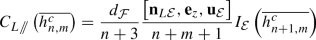
  with $d_{\mathcal {F}}=\mathbf {n}_{L\mathcal {E}}\cdot \mathbf {OA_{\mathcal {E}}}$. The sum $\sum _{\mathcal {E}\in \partial \mathcal {F}}\left[ \mathbf {n}_{L\mathcal {E}},\mathbf {e}_{z},\mathbf {u}_{\mathcal {E}}\right] I_{\mathcal {E}}$ is the integral of Eq. (13). However, we do not make this face contribution explicit in our implementation because we first sum each edge contribution (from left and right face).

For each degree and order, the contributions computed at the previous step 4 are summed over all the edges; all the terms depending on $\overline{h_{n,m}^{c}}$ are summed together to yield a scaled coefficient $\overline{C_{n-1,m}}^{*}$, while all the terms depending on $\overline{h_{n,m}^{s}}$ will yield a scaled coefficient $\overline{S_{n-1,m}}^{*}$.

The ratio between the normalized coefficients, $\overline{C_{n,m}}$ and $\overline{S_{n,m}}$, and the scaled coefficients, $\overline{C_{n,m}}^{*}$ and $\overline{S_{n,m}}^{*}$, is deduced from the mathematical expression of the integrals

$$\begin{aligned} \frac{\overline{C_{n,m}}}{\overline{C_{n,m}}^{*}}=\frac{\sqrt{\left( n+m+1\right) }}{\sqrt{\left( 2n+1\right) \left( 2n+3\right) }\sqrt{\left( n-m+1\right) }}\frac{a^{3}}{V} \end{aligned}$$

where V is the total volume of the considered polyhedron. The same relation holds for $\overline{S_{n,m}}$ and $\overline{S_{n,m}}^{*}$.

References

Balmino G (1994) Gravitational potential harmonics from the shape of an homogeneous body. Celest Mech Dyn Astron 60(3):331–364
Chao BF, Rubincam DP (1989) The gravitational field of Phobos. Geophys Res Lett 16(8):859–862
Chen C, Chen Y, Bian S (2019) Evaluation of the spherical harmonic coefficients for the external potential of a polyhedral body with linearly varying density. Celest Mech Dyn Astron 131(2):8
De Loera JA, Dutra B, Köppe M, Moreinis S, Pinto G, Wu J (2013) Software for exact integration of polynomials over polyhedra. Comput Geom 46:232–252
Domingue DL, Cheng AF (2002) Near earth asteroid rendezvous: the science of discovery. Johns Hopkins APL Tech Digest 23(1):6–17
Forsberg R (1993) Modelling the fine structure of the geoid: methods, data requirements and some results. Surv Geophys 14:403–418
Heiskanen WA, Moritz H (1967) Physical geodesy. WH Freeman and Company, San Fransisco
Jamet O, Thomas E (2004) A linear algorithm for computing the spherical harmonic coefficients of the gravitational potential from a constant density polyhedron. In: CNES (ed) Proceedings of the 2nd international GOCE user workshop, GOCE, the geoid and oceanography
Lasserre JB (1999) Integration and homogeneous functions. Proc Am Math Soc 127(3):813–818
Martinec Z, Pěč K, Burša M (1989) The Phobos gravitational field modeled on the basis of its topography. Earth Moon Planets 45:219–235
Miller J, Konopliv A, Antreasian P, Bordi J, Chesley S, Helfrich C, Owen W, Wang T, Williams B, Yeomans D, Scheeres D (2002) Determination of shape, gravity, and rotational state of asteroid 433 eros. Icarus 155(1):3–17
Nagy D, Papp G, Benedek J (2000) The gravitational potential and its derivatives for the prism. J Geod 74(7–8):552–560
Pawlowski RS, Hansen RO (1990) Gravity anomaly separation by Wiener filtering. Geophysics 55(5):539–548
Romberg W (1955) Vereinfachte numerische integration. Det Kongelige Norske Videnskabers Selskab Forhandlinger 28(7):30–36 Trondheim
Tsoulis D (2012) Analytical computation of the full gravity tensor of a homogeneous arbitrarily shaped polyhedral source using line integrals. Geophysics 77(2):F1–F11
Tsoulis D, Jamet O, Verdun J, Gonindard N (2009) Recursive algorithms for the computation of the potential harmonic coefficients of a constant density polyhedron. J Geod 83(10):925–942
van Rossum G, Drake FL (2011) The Python language reference manual. Network Theory Ltd, Boston
Werner RA (1997) Spherical harmonic coefficients for the potential of a constant-density polyhedron. Comput Geosci 23(10):1071–1077
Wieczorek MA, Meschede M (2018) Shtools: tools for working with spherical harmonics. Geochem Geophys Geosyst 19(8):2574–2592
Acknowledgements
This study was partly supported by IdEx Université de Paris ANR-18-IDEX-0001. IPGP contribution number is 4055.
Author information
Authors and Affiliations
Contributions
This research was jointly designed by OJ and DT; OJ found the mathematical relations and performed their implementation; and OJ and DT analyzed the results and wrote the paper.
Corresponding author