


Introduction
Determining rates of subglacial erosion is difficult due to the challenges involved in accessing the beds of glaciers and often requires relying upon proxy data rather than direct measurement (Hallet and others, Reference Hallet, Hunter and Bogen1996). Boreholes and slab experiments (e.g. Lappegard and Kohler, Reference Lappegard and Kohler2005; Iverson and others, Reference Iverson2007) allow for the direct measurement of erosion rates but only provide data over short-timescales (on the order of years) and must be repeated at numerous locations under a glacier to reveal spatial patterns of erosion. Techniques that examine glacial sediment volumes allow one to estimate erosion over much longer timescales (on the order of thousands of years or more) but are heavily dependent on subglacial and proglacial hydrology (e.g., Riihimaki and others, Reference Riihimaki, MacGregor, Anderson, Anderson and Loso2005) and cannot capture high-resolution spatial variations in erosion rates. Given the variable magnitude and possibly discontinuous nature of glacial erosion (Hooyer and others, Reference Hooyer, Cohen and Iverson2012), care must be taken in scaling erosion rates to the time and spatial scales of interest for landscape evolution (e.g., Koppes and Montgomery, Reference Koppes and Montgomery2009). Better constraints on the magnitude of subglacial erosion on timescales longer than those of a single erosive event, but shorter than those of a full glacial cycle will aid in modeling the history of glacial and post-glacial landscapes (e.g., Harbor, Reference Harbor1992; Herman and others, Reference Herman, Beaud, Champagnac, Lemieux and Sternai2011). Understanding the spatial distribution of erosion underneath glaciers better would improve interpretations of the landscapes created by glacial erosion.
We measured in situ cosmogenic carbon-14 (14C) and beryllium-10 (10Be) concentrations in samples of glacially eroded bedrock exposed in the forefield of Engabreen, Norway (Fig. 1). The relationship between 14C and 10Be concentrations allows us to estimate the integrated duration of ice cover at our site during the Holocene and erosion depths over that duration. As we will show, nuclide concentrations indicate a very short (~1 ka) total burial duration with implications regarding the timing of erosion at the site. In particular, the in situ 14C–10Be ratio in our samples indicates that plucking and abrasion took place during the most recent period of ice cover, likely the Little Ice Age.

Fig. 1. Maps displaying the location of our study site on regional to local scales. Orthophotographs and maps in parts A and B courtesy of © Kartverket. (a) Map showing the part of coastal Norway in which Engabreen is located. (b) Mosaiced orthophotos of the region surrounding our study site depicting Engabreen, Engabreevatnet and Holandsfjorden to the north. The approximate location of a farm overrun by a glacier advance about 1723 CE (Karlén, Reference Karlén1988) is also shown. The dominant foliation direction of the forefield bedrock is visible as color banding. (c) Satellite image of the Engabreen forefield, which contains our study site. Sample locations are marked with green circles and labeled with corresponding sample numbers. The red arrow indicates the direction of ice flow. Slope-perpendicular Nye channels appear above and to the right of the glacier in the image as dark, linear features. The main outlet channel draining Engabreen is visible as a light linear feature extending from the toe of the glacier to the upper left corner of the image.
Cosmogenic-nuclide measurements can be made at multiple locations in a glacial forefield with relative ease, as samples can be collected from exposed bedrock. Our cosmogenic nuclide technique bridges the gap between the short- and long-term scales examined by other methods and improves spatial resolution and coverage by allowing us to target specific glacial features.
Background
Cosmogenic nuclides such as 14C and 10Be are products of the interaction of secondary cosmic ray particles (neutrons, protons and muons) with matter at or near the surface of the Earth. Cosmic rays are attenuated exponentially by the matter through which they pass. Furthermore, different production pathways have different attenuation lengths and therefore depth dependences (Gosse and Phillips, Reference Gosse and Phillips2001). Neutrons emitted by the most productive pathway at the Earth's surface, spallation, are rapidly attenuated with depth and thus produce a negligible number of nuclides below ~5 m of bedrock. Other production pathways such as muon capture produce nuclides at the Earth's surface at a far lower rate than spallation does but are much less rapidly attenuated with depth. Production at depths from ~5–100 m therefore is dominantly by muons (e.g., Gosse and Phillips, Reference Gosse and Phillips2001; Balco, Reference Balco2017).
The concentration of a cosmogenic radionuclide increases with the duration and degree of exposure until ultimately reaching secular equilibrium, the state in which production of nuclides is balanced by loss to radioactive decay and erosion. In its simplest case, the exposure age of a sample is therefore proportional to the concentration of a given nuclide (Lal, Reference Lal1991). Short episodes of burial (e.g., by ice or sediment), however, may only partially deplete nuclide concentrations when production effectively ceases but decay continues, leaving a rock with ‘inheritance’ (i.e., nuclides produced during one or more previous episodes of exposure). Therefore, events in the history of a sample alter the concentrations and ratios of nuclides in a rock surface in characteristic ways. In a two-radionuclide system, halting nuclide production in a sample (e.g., burial) will modify nuclide ratios in favor of the longer-lived nuclide. Removing nuclides through erosion will also alter these ratios but in favor of the nuclide with a longer effective attenuation length. Analyzing multiple cosmogenic nuclides with different half-lives potentially allow one to identify and resolve the erosive and exposure histories of a sample.
Here we use 10Be and 14C to examine the exposure and erosion history of a glacial forefield. 10Be is a frequently used nuclide for exposure dating with a 1.394 Ma half-life, which sets its effective usable range on the order of centuries to millions of years (Chmeleff and others, Reference Chmeleff, von Blanckenburg, Kossert and Jakob2010). 10Be is commonly used on account of the relative ease of its isolation and measurement. 14C, with its much shorter 5.7 ka half-life (Olsson, Reference Olsson1968), is a useful nuclide to pair with 10Be to identify burial episodes and erosion on Holocene timescales (Lal, Reference Lal1991). The production rate of 10Be is more strongly attenuated than the production rate of 14C is, which aids in the estimation of the magnitude and timing of erosion. For example, the nuclide ratio in a sample at depth, exposed by a plucking event, will be rapidly overprinted by production at the surface rate. In an exposed sample a measured nuclide ratio indicative of production at depth implies that the plucking event which exposed it must have been recent.
Setting
Engabreen is an outlet glacier of the Svartisen ice cap in coastal northern Norway (Fig. 1). During the Pleistocene, the ice cap was overrun by and formed a part of the Scandinavian ice sheet (Olsen, Reference Olsen2002). Marine shells from terminal moraines at nearby Fonndalen date to 11 990 ± 60 14C years BP (Olsen, Reference Olsen2002; 13 400 ± 70 cal. yr BP, calibration curve MARINE13, http://calib.org), indicate that glaciers terminated near the current fjord shore at the beginning of the Younger Dryas. We assume that the glacier occupied a similar position following the Younger Dryas. The outermost moraine between the current terminus of Engabreen and Holandsfjorden is tentatively dated to about 1200 CE (Worsley and Alexander, Reference Worsley and Alexander1976) and historical records of ice advance (Karlén, Reference Karlén1988) show that the Engabreen terminus was several kilometers longer and terminated near sea level in historic times. The terminus has since retreated to ~200 m a.s.l., exposing a bedrock forefield consisting dominantly of amphibolite and biotite garnet schists (Sigmond and others, Reference Sigmond, Gustavson and Roberts1984). The dominant bedrock foliation strikes perpendicular to sub-perpendicular to ice flow. In general, the bedrock surface is polished and striated, and many areas display crescentic gouges and plucking (Fig. 2). The forefield has a stepped habit descending as a series of rounded ridges or benches separated by numerous channels ranging from a few centimeters to several meters deep, interpreted as Nye channels by Messerli (Reference Messerli2015).

Fig. 2. (a) Example of a crescentic gouge filled with rainwater from site EG10-13 (on the lower transect). The curved face of the gouge bows downhill. Boot for scale. (b) Example of a plucked face near site EG10-06 (on the upper transect). Boot for scale. (c) Up-valley view of the Engabreen forefield consisting of orthophotographs draped over a digital terrain model. Sample sites from which data were used in this study are displayed as white circles labeled with sample names (‘EG’ has been excised from labels for clarity). The main Nye channel draining Engabreen can be seen at right. Note the stepped nature of the forefield, especially on the lower left of the image. Orthophotographs courtesy of © Kartverket.
We make several assumptions about Engabreen: that glacial cover and erosion during the Last Glacial Maximum was sufficient to decrease cosmogenic 10Be and 14C concentrations in the bedrock of our study site below detection limits and that any subaerial erosion or rock uplift was negligible over the timescales in question. Additionally, we assume that snow cover at our sites is transient (Theakstone, Reference Theakstone2013) as the maritime climate at Engabreen causes temperatures to regularly rise above freezing, even during the winter months and the ground is commonly free of snow by mid-spring (Andreassen and others, Reference Andreassen2006).
Methods
We sampled along two transects in 2010 CE – one ~200 m from the Engabreen terminus at ~150 m a.s.l. and the other ~500 m from the terminus at ~20–30 m a.s.l. All sites were exposed within the two years prior to sampling. Samples were collected from exposed surfaces with a hammer and chisel. Topographic shielding was measured at each sample site by measuring the azimuth and inclination of horizon obstructions in a full circle around each sample. Topographic shielding corrections as well as sample location and size data are presented in Table 1.
Table 1. Sample locations and parameters

Our sample transects generally span the forefield from the right-lateral valley wall to near the middle of the valley. We assume that samples from a given transect have the same exposure history (e.g., the in-transect differences are minimal on a millennial timescale) because the transects extend perpendicular to ice flow. Our sampling strategy, which targeted sites atop bedrock ridges and rises, lends us confidence that no substantial postglacial erosion of the sample surfaces was carried out by streams, which preferentially flow through depressed channels along foliation planes and through former Nye channels (Messerli, Reference Messerli2015). This strategy additionally minimizes the effect of transient till cover at our sites, as loose sediment on local topographic highs would be preferentially transported to lows by gravity.
Samples were crushed, quartz fractions isolated and divided into aliquots for 10Be and 14C analysis. Aliquots for 10Be analysis were dissolved in concentrated HF and HNO3, ~0.25 mg 9Be added, and Be isolated from other ions by ion exchange chromatography at the Tulane University Cosmogenic Nuclide Laboratory (TUCNL). 10Be–9Be ratios were determined via accelerator mass spectrometry (AMS) at the Purdue Rare Isotope Measurement Lab (PRIME). 14C extraction was carried out at TUCNL following methods outlined in Goehring and others (Reference Goehring, Wilson and Nichols2019). Briefly, the sample is fused in LiBO2 for one hour at 500°C to remove potential surface contaminants and then held for 3 hours at 1100°C; released C-species are oxidized to form CO2, which is then purified and graphitized via H2 reduction in the presence of Fe. 14C–13C ratios were measured at the National Ocean Science Accelerator Mass Spectrometry (NOSAMS) facility. Stable C isotope ratios were measured at the University of California, Davis Stable Isotope Facility. Data reduction followed Hippe and Lifton (Reference Hippe and Lifton2014).
We scaled sea level, high latitude production rates from the calibration dataset of Stroeven and others (Reference Stroeven2015) to our sample sites using the scaling scheme of Stone (Reference Stone2000) and muon scaling follows that in Balco (Reference Balco2017). Due to the high latitude, low elevation location of our samples, this scaling scheme is appropriate. Alternate scaling schemes, such as that of Lifton and others (Reference Lifton, Sato and Dunai2014), alter our scale factor by less than 1%.
14C–10Be isochrons
Here, we follow the logic detailed in Goehring and others (Reference Goehring, Muzikar and Lifton2013) to determine the exposure duration and erosion depth of our samples. We modeled the attenuation of 10Be production with depth via the following equation:

in which P 10(z) is the 10Be production rate at depth z (z = 0 denotes the surface) and φ a term denoting the depth dependence of 10Be production. φ(z) typically takes the form of a negative exponential as production decreases with increasing mass depth. As discussed above, 14C production differs in terms of depth dependence with respect to 10Be and is furthermore dependent on the cosmic ray spectrum at a site. We account for this by introducing the parameter β which relates the depth dependence of 14C to 10Be, and we can therefore define the production rate of 14C at depth by

in which P 14(z) is the 14C production rate at depth z and P 14(0) is the 14C surface production rate. Where β = 1, the 14C and 10Be production rates are equally attenuated by depth. Where β < 1, the 14C production rate is less attenuated than that of 10Be. Because 14C production by muons exceeds 10Be production by muons and because of the high-latitude and low-elevation location of our study site, we expect low values of β (Heisinger and others, Reference Heisinger2002a, Reference Heisinger2002b).
Measured nuclide concentrations in a given sample i are described by the following two equations:


in which N 10i and N 14i (both atoms g−1) and P 10i and P 14i (both atoms g−1 a−1) are the 10Be and 14C concentrations and scaled production rates at the surface in sample i, respectively, and T 0 the initial exposure age. λ 14 is the decay constant of 14C and t e the exposure duration of the sample. Note that the decay of 10Be is neglected here, as it would be of negligible magnitude on a millennial timescale.
Solving for φ(z) in Eqn (3) allows us to substitute this value into Eqn (4) to generate the equation for an isochron (Fig. 3):

which shows the 14C concentration (normalized to its production rate) as a function of 10Be concentration.

Fig. 3. Isochron diagram demonstrating the behavior of a two-radionuclide (beryllium-10 [10Be] and carbon-14 [14C]) system. Nuclide concentrations are normalized by dividing the production rate of that nuclide, thus the unit of these values is years. Isochrons are labeled with the burial durations they represent. It is important to note that isochrons are calculated using surface production rates and are thus approximations. Substantial erosion will expose samples that accumulated nuclides at different rates, which is why samples can plot above the t = 0 isochron. The upper transect samples with high 10Be concentrations (EG10-02 and -04) are consistent with a minimum of 2–8 ka of cover while the lower-transect samples and the upper-transect samples with low concentrations plot above the t = 0 isochron, indicating enhanced 14C production relative to 10Be. Note, however, that we do not account for glacial erosion.
In the isochron shown in Figure 3, samples will plot progressively further from the origin as nuclides accumulate during exposure, while eroding samples will lose accumulated nuclides. Samples with little to no exposure and/or which are heavily eroded will therefore plot near the origin. Due to the different half-lives of the two nuclides in question, samples buried for the same length of time will all plot along a line drawn through the origin of the graph. This line is an isochron (colored lines in Fig. 3). The slope of the line fit to unburied samples will equal the ratio of the production rates of the measured nuclide. For a buried sample, increasing burial duration decreases the isochron slope such that the line is ‘rotated towards’ the axis on which the longer-lived nuclide is plotted (for an idealized example, see Fig. S1). Note that, unless a sample is buried very deeply, it will continue to accumulate nuclides (albeit at a very low rate). Dating approaches using multiple nuclides, such as the one we use here (developed in Goehring and others (Reference Goehring, Muzikar and Lifton2013)) allow us to graphically interpret the data from our sample transects. Samples from one transect should all have the same exposure and burial history within measurement precision. We employ a Bayesian fitting method to calculate the probability density function for the exposure duration (t e) and β value of our site following Goehring and others (Reference Goehring, Muzikar and Lifton2013). This method bypasses the normal approach of fitting the isochron slope and then solving for parameter values and instead directly determines parameter values while considering a range of geologic plausibilities encapsulated in the prior probabilities for known and unknown parameters.
Erosion calculations
We numerically determine the depth to which each sample has been glacially eroded using our measured 10Be concentrations and the resulting exposure duration. The magnitude of erosion is calculated by defining φ(z) in Eqn (3) as,

in which sp indicates spallation and μ− and μf indicate negative and fast muons, respectively (i.e. P 10sp would refer to the production rate of 10Be via spallation, ${\rm \Lambda} _{\mu _f}$ the attenuation length of production by fast muons, etc.). Note that the P terms in Eqn (6) are normalized to the total surface production rate such that φ(z) is a dimensionless parameter. We solve for z numerically for each sample assuming Λsp = 160 g cm−2, ${\rm \Lambda} _{\mu _-}$
 = 1510 g cm−2 and ${\rm \Lambda} _{\mu _f}$
 = 4320 g cm−2 (Gosse and Phillips, Reference Gosse and Phillips2001; Heisinger and others, Reference Heisinger2002a, Reference Heisinger2002b) for this calculation. One-sigma uncertainties on erosion depths are determined via 500-point Monte Carlo bootstrapping.
Results
Cosmogenic nuclide concentrations
All samples yield 10Be and 14C concentrations above detection limits, indicating that the samples were exposed for sufficient time to generate an inventory and not eroded deeply enough to remove the entire inventory. The concentrations of either nuclide do not vary in a systematic way with distance along a transect perpendicular to the flow of Engabreen, but concentrations in lower transect samples are generally lower compared to concentrations in the upper transect samples (Table 2).
Table 2. Cosmogenic nuclide concentrations and apparent exposure ages
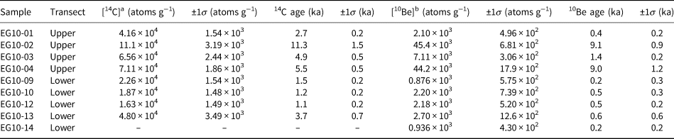
Apparent exposure ages are calculated via the CRONUS-Earth online exposure age calculator (version 3) using production rates scaled to sea level high latitude using the scaling scheme of Stone (Reference Stone2000) and corrected for topographic shielding. Note that samples EG10-13 and -14 were collected from different surfaces of the same site; EG10-13 from a horizontal surface and -14 from a lee-side vertical surface.
a Carbon-14 concentration.
b Beryllium-10 concentration.
10Be concentrations vary across the upper transect by an order of magnitude, from 2100 ± 500 atoms g−1 to 45 000 ± 680 atoms g−1 (Table 2). The samples with the highest concentrations (EG10-02 and EG10-04) are adjacent to the samples with the lowest concentrations (EG10-01 and EG10-03). Upper-transect 14C concentrations range from 42 000 ± 1500 atoms g−1 to 110 000 ± 3200 atoms g−1.
10Be concentrations for the lower transect are between 880 ± 580 atoms g−1 and 2700 ± 1300 atoms g−1 (Table 2). Lower transect 14C concentrations range from 16 000 ± 1500 g−1 to 48 000 ± 3500 atoms g−1. The proportional decrease in concentrations from the upper transect to the lower is less for 14C than it is for 10Be. Samples EG10-13 and EG10-14 are from the same location – EG10-14 was collected from a vertical lee face and EG10-13 from the stoss side of the same feature. 14C concentrations were not measured from sample EG10-14 because the sample only contained enough quartz for 10Be analysis.
Exposure history
The resulting exposure duration for Engabreen, inclusive of both transects, is 11.0 ± 0.2 ka. Given the close spatial proximity of our two transects, we calculated the exposure duration via the method of Goehring and others (Reference Goehring, Muzikar and Lifton2013) using all of our samples instead of calculating separate exposure durations for each transect. Recent and historical rates of retreat (Rekstad, Reference Rekstad1893) indicate that Engabreen is capable of retreating the ~300 m between our two transects within the 200 yr of the 1σ uncertainty on our calculated exposure duration. Subtracting the exposure duration of the transects from the initial exposure age of 12.0 kcal yr BP assumed from Olsen (Reference Olsen2002) yields a burial duration of 1.0 ± 0.2 ka. We base our T 0 assumption on the idea that shells buried under moraines near the current fjord shore closely limit the maximum initial exposure of our sample site ~2 km inland.
Erosion depths
Erosion depths vary by more than an order of magnitude along the upper transect (10 ± 1 cm, EG10-02 and -04, to 214 ± 14 cm, EG10-01) and to a lesser degree along the lower transect (184 ± 22 cm, EG10-13, to 295 ± 73 cm, EG10-09; Fig. 4, Table 3). Additionally, sites with very different erosion depths are located adjacent to one another (e.g., EG10-01 and -02).

Fig. 4. Elevation profiles of our two sampling transects looking up-glacier. Sample sites (purple circles) are shown projected onto the upper (blue line) and lower (orange line) transects. Samples are labeled with their sample name and erosion depth. The main Nye channel carrying meltwater out from below Engabreen along the left-lateral wall of the valley is denoted with a black arrow. Elevation data from the Norwegian Mapping Authority.
Table 3. Calculated erosion depths and 14C–10Be concentration ratios

Erosion depths calculated using the integrated exposure duration determined using the Bayesian isochron method. Carbon-14 concentration was not measured from sample EG10-14, so its ratio is omitted from this table.
The resulting uncertainties on erosion depths are a product of two factors (Fig. S2). The first is that the larger relative uncertainties are associated with low nuclide concentrations as a result of nonlinear effects as the total number of in situ nuclides (not concentrations) approaches the number of atoms in the process blanks. The second is that, as depth increases, any given nuclide concentration profile becomes flatter and the resulting erosion depth uncertainty larger. Thus, any given measurement precision will be compatible with a wider range of erosion depths relative to shallower parts of the concentration profile and thus the resulting uncertainty will be larger.
Discussion
The spatial distribution of glacial abrasion rates is typically characterized as being dependent on sliding velocity and modification by valley-wall drag (Hallet, Reference Hallet1979) and the effective normal stress exerted by tools (such as plucked rock fragments embedded in basal ice) on the bed of a glacier (Hallet, Reference Hallet1981). As such, abrasion rates are expected to vary approximately quadratically across valley. This ideal model of abrasion does not, at first glance, adequately describe our results. Were abrasion the dominant control on nuclide concentrations at our site, nuclide concentrations would decrease quadratically toward the centerline of the glacier where sliding velocities are greatest (Fig. 5). The lack of any such clear trend indicates that additional processes acted on the Engabreen forefield to produce the spatial pattern of nuclide concentrations we observe. Given the lack of valley-scale trend and the areal geomorphology, this indicates that localized plucking has occurred.

Fig. 5. Sliding velocity and erosion depth calculated at our sample sites. (a) Sliding velocity as predicted by the method of Nye (Reference Nye1952), which takes drag from valley walls and floor into account when calculating basal sliding velocity. We calculated these velocities given the surface velocities reported for the Engabreen terminus in Jackson and others (Reference Jackson, Brown and Elvehøy2005). The plot here shows the expected quadratic dropoff in velocity due to drag from the valley walls. (b) Calculated erosion depths vs calculated sliding velocity.
Furthermore, we observe a wide-range of 14C–10Be concentration ratios (Table 3), including samples with ratios exceeding the 14C–10Be production rate ratio (~3.76). These samples are particularly interesting because we know these sites were buried during the Little Ice Age and exposed very recently. They would thus be expected to have 14C–10Be ratios less than the production ratio. It is possible that measurement or sample preparation could account for the elevated 14C–10Be ratios, particularly given the low overall concentrations and correspondingly large uncertainties. This is especially true for the lower transect 10Be concentrations, as the total number of 10Be atoms in the process blank is a significant fraction of the measured number of 10Be atoms in a sample. However, we could not identify any systematic issues with either the 10Be or 14C measurements. Therefore, we discount measurement errors as a cause of the elevated 14C–10Be ratios. Rather, we propose that elevated production of 14C at depth by muon capture relative to 10Be and rapid deep erosion leads to the observed ratios. Because muons have longer attenuation lengths than fast neutrons do, the relative magnitude of the muon component of cosmogenic-nuclide production increases with depth while the absolute production rate decreases. Since 14C has a significantly higher production rate by muons than does 10Be (when normalized to surface production rates, the muogenic 14C–10Be production rate ratio equals ~13.62 at our sites), the 14C–10Be ratio increases with depth (Heisinger and others, Reference Heisinger2002a, Reference Heisinger2002b). As production by muons dominates production beyond depths of ~2.5 m (Briner and others, Reference Briner, Goehring, Mangerud and Svendsen2016), samples from deeply eroded sites represent rock in which 14C production was proportionally greater (compared to 10Be production) than at lesser depths (Fig. 6). The short, ~1 ka burial duration of our site requires erosion rates in excess of 2 mm a−1 to explain the highest 14C–10Be ratios exhibited by our samples (Table 3). It is unlikely that abrasion alone would erode the bedrock beneath Engabreen that quickly, as reported subglacial-abrasion rates are commonly lower than this by roughly an order of magnitude (e.g., Briner and Swanson, Reference Briner and Swanson1998; Goehring and others, Reference Goehring2011). Further, it is unlikely that the required high abrasion rates operated while sparing adjacent sampled bedrock from significant erosion. Scaling the erosion rates calculated from recently plucked sites would therefore likely overestimate long-term erosion rates for a glacier.

Fig. 6. 14C–10Be ratios of samples from the upper (blue circles) and lower (orange triangles) transects. The shallowly eroded samples of the upper transect (EG10-02 and EG10-04) have the lowest ratios and these ratios decrease with the calculated erosion depth, demonstrating the reduced attenuation of in situ 14C production with depth relative to that of 10Be. ‘EG10-’ has been excised from data labels for clarity.
Given sample surfaces that were originally at depth and the spatial heterogeneity of erosion, plucking must be invoked to explain the elevated 14C–10Be ratio. Furthermore, the plucking must have occurred during the Little Ice Age instead of during Last Glacial Maximum cover, as the 14C–10Be ratio in our samples had not re-equilibrated to the surface production-rate ratio. Figure 6 demonstrates this observation; the two deeply eroded samples of the upper transect (EG10-01 and -03) and the more deeply eroded lower transect all have high 14C–10Be ratios.
Plucking will remove evidence of past abrasion at a site. As all but one of our sites showed evidence of abrasion but some also showed evidence of plucking, the abrasion must have occurred between the plucking event and the exposure of the sample sites. Historical records and our data imply that the Engabreen forefield was uncovered for the majority of the Holocene and only buried recently. Therefore, the isotopic and geological data allow us to construct an ordered timeline of events at our plucked sites: plucking during Little Ice Age cover, abrasion during or before glacial retreat, followed by a period of exposure short enough that high 14C–10Be ratios are still preserved in exposed surfaces.
Supplementary material
The supplementary material for this article can be found at https://doi.org/10.1017/aog.2019.42.
Acknowledgements
We wish to acknowledge the Purdue Rare Isotope Measurement laboratory, the Woods Hole National Ocean Sciences Accelerator Mass Spectrometry facility and the University of California, Davis Stable Isotope Facility for sample nuclide measurements. We also thank Kristine Hippe and two anonymous reviewers for constructive reviews that improved this manuscript.
Appendix – Geochemical data tables
Table A1. Carbon-14 sample geochemical data

Process blanks
Table A2. Beryllium-10 sample geochemical data
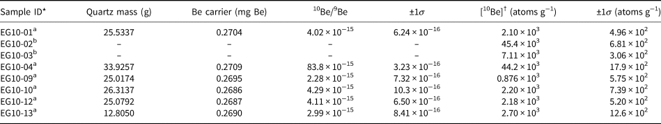
Process blanks


 Open access