An MPC-Enabled SWMM Implementation of the Astlingen RTC Benchmarking Network

Abstract

The advanced control of urban drainage systems (UDS) has great potential in reducing pollution to the receiving waters by optimizing the operations of UDS infrastructural elements. Existing controls vary in complexity, including local and global strategies, Real-Time Control (RTC) and Model Predictive Control (MPC). Their results are, however, site-specific, hindering a direct comparison of their performance. Therefore, the working group ‘Integral Real-Time Control’ of the German Water Association (DWA) developed the Astlingen benchmark network, which has been implemented in conceptual hydrological models and applied to compare RTC strategies. However, the level of detail of such implementations is insufficient for testing more complex MPC strategies. In order to provide a benchmark for MPC, this paper presents: (1) The implementation of the conceptual Astlingen system in an open-source hydrodynamic model (EPA-SWMM), and (2) the application of an MPC strategy to the developed SWMM model. The MPC strategy was tested against traditional and well-established local and global RTC approaches, demonstrating how the proposed benchmark system can be used to test and compare complex control strategies.

1. Introduction

Real-time operations of urban drainage systems (UDS) have proven to be an efficient and cost-effective management strategy for reducing pollution to the aquatic environment without having to invest in expensive infrastructural expansions [1,2,3,4,5,6]. Applied approaches include Real-Time Control (RTC), such as rule-based control (RBC) [7,8], and Model Predictive Control (MPC) [9,10,11]. However, RTC and MPC performances are site-specific and also depend on the rainfall characteristics, hindering cross-validation of control algorithms across systems and research groups. There is therefore the need for a common method for comparing RTC and MPC approaches in order to support further advancements and widespread application of these technologies in both academia and practice [12]. Under this necessity, the working group ‘Integral Real-Time Control’ of the German Water Association (DWA) has constructed the Astlingen example network [5], which serves as a benchmark complementing the German DWA-M180 document on planning of RTC systems [6]. The purpose of a benchmarking model was to encourage as many experts (researchers, practitioners) as possible to use and compare performance of different control methodologies under the same test bed. Therefore, the Astlingen benchmark model should preferably also be implemented in a free, widely used open-source software.

Currently available implementations of the Astlingen network are based on simple hydrological models. For example, the hydrological module of the Simba# simulator has previously been used to demonstrate the base case (BC) of locally controlled throttle settings, as well as the global rule-based equal-filling-degree (EFD) approach [13]. MPC has been widely investigated for UDS optimization solutions [1,3,4,7,9,10,11,14,15,16,17], but it is difficult to find a contribution with clear definition of the internal MPC model, as well as the core implementation principles [11]. Therefore, the extension of the benchmark model for MPC application and testing can support the development of these techniques. Furthermore, testing MPC often requires more complex description of the hydraulic processes taking place in the network (e.g., backwater effects). Therefore, simple conceptual hydrological models might be inadequate.

This paper presents an implementation of the Astlingen case based on a hydrodynamic Storm Water Management Model (SWMM). EPA-SWMM 5.1.013 [18] is a free, open-source software that is widely used in both academia and practice, thereby making the Astlingen benchmark case available to a wider audience. The SWMM model was calibrated to emulate the results from the Simba# model implementation, which was used as reference in this paper [5,19]. The SWMM implementation was combined with an MPC strategy to provide an example of a detailed description of the methods and core principles of an MPC application for UDS control. The MPC controller was defined by two aspects: The internal model and the control design. The internal model used a simplified discrete model of the Astlingen system, while the control design defined the behavior of the system and the length of each prediction. The MPC optimization was defined by the conceptual network of Astlingen, while the effects of the generated control setpoints were simulated in the SWMM model. In order to integrate the optimization and simulation process, a closed-loop RTC scheme wrapped in PySWMM (a Python-based SWMM Software) was also provided. A one-year simulation was used to evaluate the MPC approach, which was compared against two control scenarios: Base case (BC) and EFD.

To facilitate the wide usage of the results from this article for benchmarking, teaching, research and development, all the data, models, and codes used for the examples can be freely accessed on https://github.com/open-toolbox/SWMM-Astlingen.

2. SWMM Model and Rule-based Control

2.1. The Astlingen Benchmark System

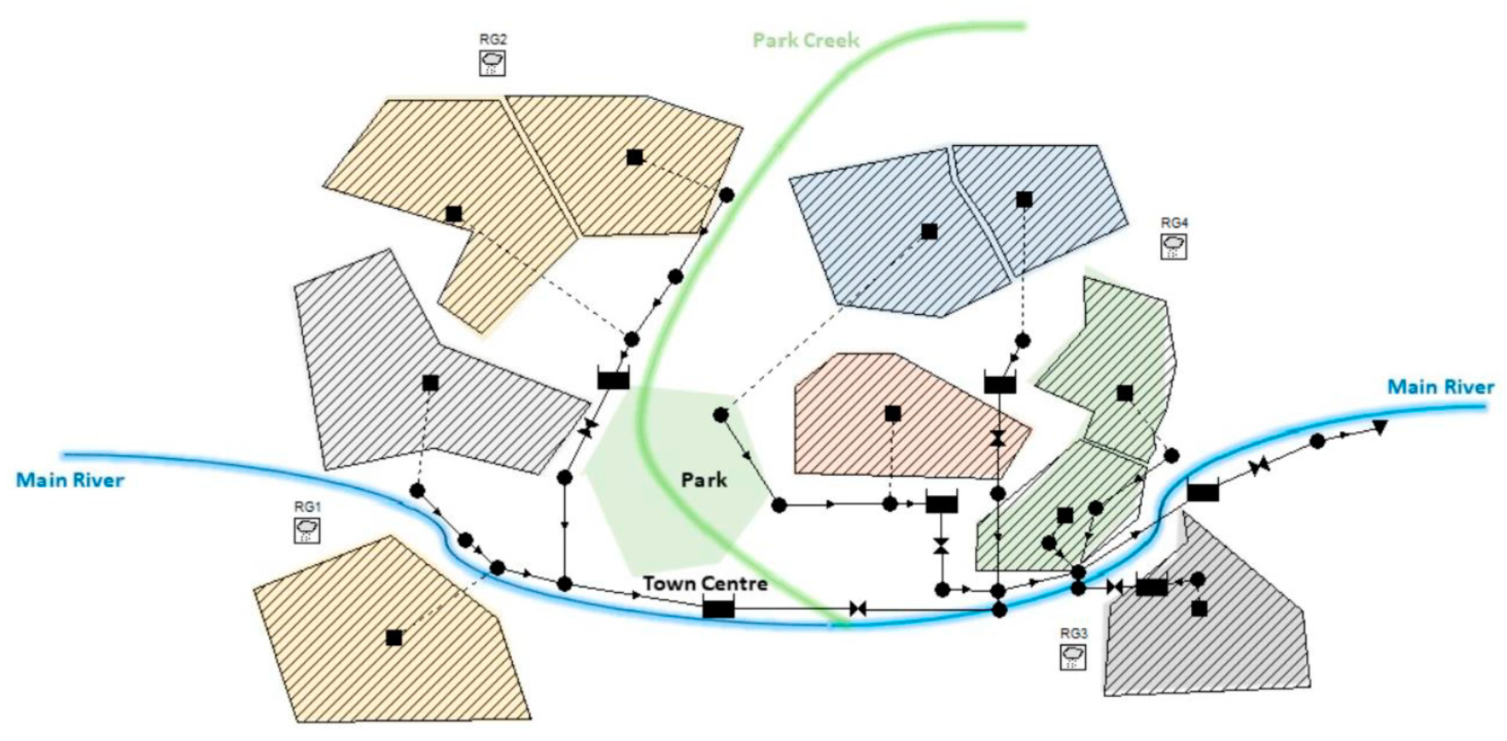
The Astlingen benchmark system [5,18] is a hypothetical case area including both combined and separated sewer systems. The schematic representation of the Astlingen network is presented in Figure 1 (adapted from [5]). Rainfall spatial heterogeneity is included using four rainfall gauges, connected to 10 subcatchments (SC). The system includes six storage tanks (where Tank 1 and 5 are not controlled) with a total storage volume of 5900 m³. There are 10 combined sewer overflows (CSO): One for each storage basin (CSO1-6) and four at junction nodes (CSO7-10). Flow routing and transport across the network are represented by time delays (ranging from a minimal 5-minute to a maximal 20-minute). The documentation provided by the working group ‘Integral Real-Time Control’ of the German Water Association (DWA) also includes additional information on the network layout, overflow structures, as well as 10-year rainfall data [20]. These are provided as four rainfall series based on measurements provided by the Erftverband water utility (Germany) with a five-minute time resolution [19,20]. The average annual rainfall at these four rainfall stations amounts to 705 mm, 723 mm, 699 mm, and 711 mm, respectively, and an overview of the first year rainfall of data is shown in Figure S1(Supplementary Materials). Two receiving bodies are defined for the CSOs, which are the Main River and the smaller but more sensitive Park Creek.

2.2. Model building

The SWMM model was built to emulate the results from the implementation in Simba# presented in [5], which was used as reference. Implementing the Astlingen benchmark network in the detailed hydrodynamic SWMM model requires a series of assumptions, since the original system has been described with a level of details suitable for a simple hydrological model. These assumptions include the definition of physical details of the system, such as system setup and geometric elements between tanks. The criteria used to build the SWMM model and to define its elements were:

• The deviation between the outputs provided by SWMM and Simba# models should be less than 10%. This comparison was based on a one-year simulation with both models.
• The number of additional elements added to the detailed model should be kept to a minimum.

The detailed SWMM model was developed by following a three-step procedure: (1) Rainfall-Runoff Calibration, to estimate the subcatchments parameters; (2) Base Case Calibration, to configure and estimate the parameters of the new elements added in the detailed models; (3) EFD Verification, to ensure that the detailed model achieve the same results as the conceptual when applied for testing control strategies.

2.2.1. Rainfall-Runoff Calibration

In the conceptual Simba# model of Astlingen, rainfall-runoff flows are calculated using Linear Reservoir Models with the parameters n = 3 (number of tanks) and k = 5 minutes (reservoir constant).

SWMM conceptualizes a subcatchment as a rectangular surface with uniform slope S (-) and width W (m), draining to a single outlet channel. The relative runoff flow Q [m/s] from this subcatchment was computed using the Manning equation expressed as (see [21] for further details):

$$Q=\frac{1}{Ae}W{S}^{1/2}{d}^{5/3}$$

(1)

where A $\left[m^2\right]$ is the impervious area, e (s/m^1/3) is the impervious area roughness, d (m) is the net depth excess ponds atop the subcatchment surface. Considering that A for a subcatchment is a constant defined in the conceptual model, the parameters to be estimated are W, S, and e. These were estimated by a trial and error procedure, comparing the simulated runoff from SWMM against the one from Simba#. The parameters were calibrated until a Nash–Sutcliffe Efficiency [22] above 0.65 was reached, and the parameter set which generate the best fitting was used (

Table 1. SWMM rainfall-runoff parameters estimated for the 10 subcatchments in Astlingen.

Subcatchment	A (ha)	W (m)	S (-)	e (s/m1/3)
SC01	33.00	2400	0.80	0.009
SC02	22.75	1500	0.80	0.009
SC03	18.00	2000	0.50	0.007
SC04	6.90	200	0.70	0.009
SC05	15.60	1000	0.50	0.007
SC06	32.55	985	0.50	0.010
SC07	4.75	360	0.51	0.020
SC08	28.00	1950	0.45	0.010
SC09	6.90	650	0.40	0.016
SC10	11.75	650	0.50	0.008

). An example of the simulated runoff from the 10 subcatchments is shown in Figure S2 (Supplementary Materials).

2.2.2. Base Case Calibration

The BC scenario is based on local controls which uses constant nominal throttle flow settings. Six orifices are used to control the emptying of each storage tanks, which are the only controllable elements in the Astlingen network. These directly affect the CSO volumes from the overflow structures located at basins (CSO1-6), and indirectly the volumes discharged at the junction nodes (CSO7-10). The latter are also affected by the characteristics of the upstream network (e.g., flow input and the routing abilities). Therefore, the throttle settings, as well as the physical characteristics of the nodes, orifices, and related pipes, were estimated by comparing the CSO volumes simulated by the two models. Similar to the Rainfall-Runoff Calibration, the parameters were estimated using a trial and error procedure until deviation between SWMM and Simba# output was below 10%.

2.2.3. Equal-Filling Degree Verification

The EFD approach is a simple illustrative example of a global RBC strategy, which compares the filling degree of the storage tanks in the network and sets the throttle flows emptying the tanks accordingly, aiming at establishing an equal filling degree in all the tanks [23]. EFD is among the control algorithms implemented in the conceptual Simba# model, where additional aspects of sensor and control delays, rainfall predictions, etc., are deliberately not considered. The EFD was also implemented in the SWMM implementation of Astlingen in order to verify its applicability for testing control strategies and to compare the estimated improvements in CSO volumes against those estimated by the Simba# implementation.

To implement EFD in the SWMM model, the control editor embedded in EPA-SWMM was used with the defined rules of comparing filling degrees for the Tank 2, 3, 4, and 6. If the water levels at these tanks were all lower than the threshold value of 20%, the nominal throttle flows values defined for the BC were used. Otherwise, the minimal possible flows were used to increase the storage in tanks with low filling, while the maximum possible flows were used for emptying tanks with high filling.

3. Model Predictive Control

MPC consists of receding horizon optimizations based on predictions from an internal model of the system to be controlled and a control design. The internal model is usually a simplified discrete representation of the internal dynamics of the system to be controlled. The control design defines the desired behavior of the controlled system, the optimal behavior, and the length of each prediction.

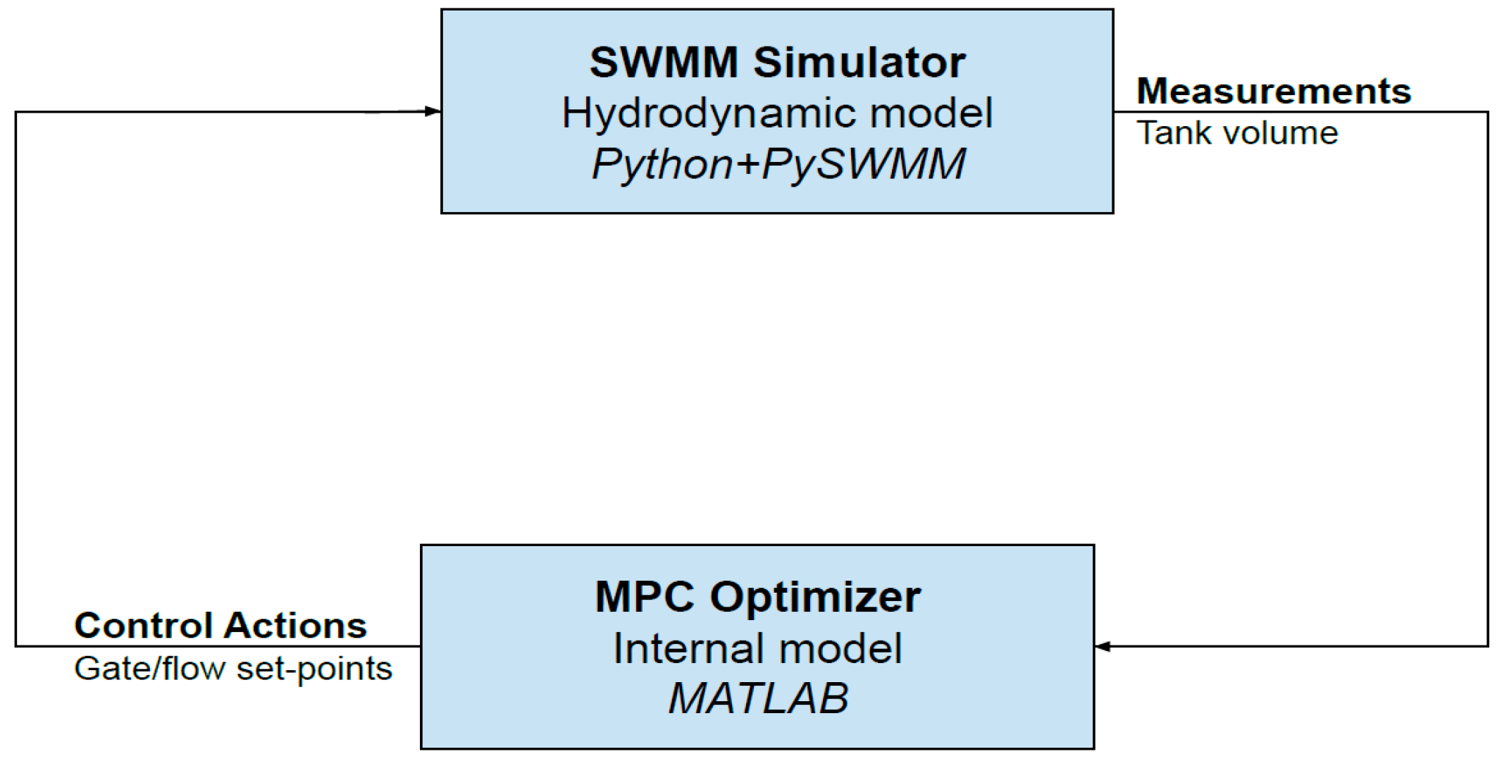
The MPC in this contribution utilizes a simplified conceptual model of Astlingen as its internal model, with the assumption of perfect forecast, generated by precomputed simulations. The MPC sampling time was 5 min, with prediction and control horizons chosen of 100 min. The MPC was implemented in MATLAB, which communicated to the detailed SWMM model through PySWMM. In order to integrate the optimization and simulation processes, a closed-loop scheme of MPC and SWMM was used (Figure 2). At each time step, the MPC optimizer (quadratic program solver from Mosek’s Matlab toolbox) generated optimal control actions and sent them as setpoints to the simulator, which fine-tuned them, computed the effects of these control actions, and updated state measurements, which were used to initialize a new optimization in the following time step. A similar scheme can be used for other RTC approaches.

3.1. Internal model

The internal MPC model includes the elements of the Astlingen system described in Figure 1, and it was built by utilizing a modular approach of well-defined sewer structures. These modules included a linear reservoir tank with a passive outflow, linear reservoir tank with a controlled outflow, and pipe with delays. The approach used for modelling weir overflow in this paper was an approximation approach through a penalty [24]. The CSOs were treated as optimization variables with a heavy cost for minimizing their use.

3.1.1. Linear Resevoir Tank—Passive outflow

The module describing the linear reservoirs or tanks at the k-th time step was based on water volume-balance:

$$\begin{array}{c}{V}_{k+1}=\left(1-\Delta T\beta \right)V_k+\Delta T\left(q_k^{in}-q_k^w\right)\end{array}$$

(2)

$$q_k^{out}=\beta V_k$$

(3)

In the case of a tank with a passive outflow, the tank volume vector is defined by the current volume $V_k\in {ℝ}^{n_p}$ (m³), the total inflow $q_k^{in}\in {ℝ}^{n_f}$ to the tank (m³/s), and the weir overflow of the tank $q_k^w\in {ℝ}^{n_p}$ (m³/s), where $\Delta T$ is the sampling time (s), $n_p,n_f$ are the numbers of the tanks and pipes (-), respectively. This relation is given by the process in Equation (2). The tank outflow in Equation (3) is a linear approximation, defined by the volume-flow coefficient $\beta =\frac{{\overline{q}}^{out}}{\overline{V}}$ [25].

$$0\le \left(1-\Delta T\beta \right)V_k+\Delta T\left(q_k^{in}-q_k^w\right)\le \overline{V}$$

(4)

$$0\le q_k^w$$

(5)

The module was further defined by the constraints on the volume and the overflow given in Equations (4) and (5), where the vector $\overline{V}$ represents maximal storage capacities of the tanks. This module was used to describe Tank 1 and 5, whose emptying orifices were passive and uncontrollable.

3.1.2. Linear Reservoir Tank—Controlled outflow

The module for the linear reservoirs with a controlled outflow was formulated in a similar manner to the passive outflow variant.

$$V_{k+1}=V_k+\Delta T\left(q_k^{in}-q_k^u-q_k^w\right)$$

(6)

$$q_k^{out}=q_k^u$$

(7)

The difference in the formulations is that the volume now also depends on the control flow $q_k^u$, and the outflow is the control flow as seen in Equations (6) and (7).

$$0\le V_k+\Delta T\left(q_k^{in}–q_k^u-q_k^w\right)\le \overline{V}$$

(8)

$$0\le q_k^u\le \beta V_k$$

(9)

$$q_k^u\le {\overline{q}}^u$$

(10)

$$0\le q_k^w$$

(11)

The constraints of this module cover the limits to the tank volume, as well as the limits to the control flow, as seen in Equations (8)–(11). The controlled outflow in the Astlingen model were all orifice-based, and were therefore dependent on the volume of the tank. For the module, this resulted in two upper constraints for the control flow, one being the linear volume-flow relation discussed previously and the second being the physical limit of the outflow pipe.

3.1.3. Pipe with Delays

The interconnection between the tanks in the Astlingen model consist of pipes. Depending on the length of the pipes, the time it takes to flow from one tank to arrive in another tank might exceed the sampling time of the model $\Delta T$. For these pipes, we introduced a delay module corresponding to one sampling time $\Delta T$.

$${\eta }_{k+1,i}=q_{k,i}^{in}$$

(12)

$$q_{k,i}^{out}={\eta }_{k,i}$$

(13)

The outflow of the module is then equal to the delay flow $\eta$, as seen in Equations (12) and (13), and the delay between tanks can be constructed as a cascade of delay modules, e.g., a 15-min delay would correspond to three delay states in succession.

Based on the different modules, it was possible to generate the entire model by connecting the right inflows and outflows together from each module. The inflow to each subpart can be seen in

Table 2. Inflows to the different elements of the systems.

Subpart	Inflow
$T_1$	$q_{k,{\eta }_{1:5}}^{out}$
$T_2$	$w_{k,2}$
$T_3$	$w_{k,3}+q_{k,{\eta }_{3:5}}^{out}$
$T_4$	$w_{k,4}$
$T_5$	$w_{k,5}$
$T_6$	$w_{k,6}$
${\eta }_{1:5}$	$q_{k,T_2}^u+q_{k,{\eta }_{1:10}}^{out}$
${\eta }_{1:10}$	$w_{k,1}+q_{k,T_3}^u+q_{k,T_4}^u+q_{k,{\eta }_{1:15}}^{out}$
${\eta }_{1:15}$	$q_{k,T_5}^{out}$
${\eta }_{3:5}$	$q_{k,{\eta }_{3:10}}^{out}$
${\eta }_{3:10}$	$q_{k,{\eta }_{3:15}}^{out}$
${\eta }_{3:15}$	$q_{k,T_6}^u$

, where the i-th runoff inflow is noted by $w_{k,i}$, and the i-th tank is noted by $T_i$. The delay flow to the i-th tank is given as ${\eta }_{i:j}$, where $j$ is the total remaining delay in minutes to the tank. The outflow of subpart z is written as $q_{k,z}^{out}$.

3.2. Control Design

The design of the MPC [26] utilized in this work was based on the model discussed above. The operational objectives for the system utilized in the MPC design in this work were:

• Maximizing flow to the WWTP ($q_{k,T_1}^{out}$);
• Minimizing CSO flow to the river/creek;
• Minimizing roughness of control.

The first objective can be achieved by a linear negative cost on the outflow of Tank 1, while the second objective can be formulated as a linear positive cost on the total overflow of the system. These objectives are collectively written as vector ${\mathit{z}}_k$. The third objective of control roughness aims for smooth control and can be written as a quadratic cost on the change in control flow. Due to the overflow being modelled by an approximation approach, a fourth objective of minimizing the accumulated overflow volume ${\mathit{V}}_k^w$ was needed.

$$J=\underset{{\mathit{q}}^u,{\mathit{q}}^w}{\min }{\displaystyle \sum _{k=0}^{Hp}}{\Vert \Delta {\mathit{q}}_k^u\Vert }_R^2+{\mathit{Q}}^T{\mathit{z}}_k+{\mathit{W}}^T{\mathit{V}}_k^w$$

(14)

$$\mathit{z}={\Phi }_{Con}{\mathit{q}}^u+\Psi {\mathit{V}}_0+\Theta \mathit{w}+\Gamma {\mathit{q}}^w$$

(15)

$${\mathit{V}}_k^w={\displaystyle \sum _{i=0}^k}\Delta T{\mathit{q}}_i^w$$

(16)

$${\Omega }_{Con}{\mathit{q}}^u+{\Omega }_{vol}{\mathit{V}}_0+{\Omega }_{rain}\mathit{w}+{\Omega }_{weir}{\mathit{q}}^w\le \mathbf{\Omega }$$

(17)

By utilizing the internal model over the prediction horizon Hp, the cost function of the MPC can be written as in Equation (14), where ${\Vert \mathbf{X}\Vert }_R^2$ is the weighted quadratic norm ${\mathit{X}}^{T}R\mathit{X}$, while the predicted objectives $\mathit{z}$ and overflow volumes, given by Equations (15) and (16), were derived from the internal model and propagation through the predicted volumes and delays. The constraints of the internal model can similarly be collected into a single matrix inequality given by Equation (17). The matrices $\Psi ,\Phi ,\Theta$, and $\Gamma$ define the influence of the initial volume, the predicted control ${\mathit{q}}^u$, inflow $\mathit{w}$, and CSO ${\mathit{q}}^w$ on the objectives, respectively. The weighting of the different objectives in the cost function was done in accordance with the approximation approach [27]. The fourth objective (minimizing accumulated CSO volume) has to have a high cost relative to all other objectives, and upstream CSOs (discharging to the more sensitive creek) have higher cost than downstream. The priority of the different objectives was given in the following order from highest to lowest priority:

• Minimization of accumulated CSO volume (16);
• Minimization of CSO to the river/creek;
• Maximizing flow to the WWTP;
• Minimizing roughness of control.

The weighs for the accumulated overflow volume from each tank are given in

Table 3. Cost function weighting of accumulated overflow volum $\mathit{W}$, showing a higher cost for upstream tank modules discharging to the sensitive creek.

Tank 1	Tank 2	Tank 3	Tank 4	Tank 5	Tank 6
1000	5000	5000	5000	5000	10,000

, while the weights of the remaining objectives are:

• 2 for the flow to the river/creek
• −1 for the flow to the WWTP
• 0.01 for the roughness of the control.

These weights indicate that the avoidance of the flow to the river and creek is prioritized twice as high as increasing flow to the WWTP. The weight on the roughness indicates the desire for the control to be smooth, but not a general priority. As seen from Table 3, the priority of the accumulated overflow can be inferred to be significantly higher than the other objectives, given the weights and the overflow volume/flow relation given by Equation (16).

4. Results

4.1. Detailed Model of Astlingen

4.1.1. SWMM Implementation

The implementation of the Astlingen benchmark network in the detailed hydrodynamic SWMM model is shown in Figure 3. The SWMM model and the reformatted rainfall series, as well as the defined EFD control rules, can be downloaded through https://github.com/open-toolbox/SWMM-Astlingen and applied directly through EPA-SWMM with different RTC approaches configured by interested practitioners.

4.1.2. Base Case Scenario

As described in the Section 2.2.2, the BC scenario was used to compare the results from the detailed SWMM model against the reference conceptual model in Simba#.

Table 4. Simulated throttle flow (reported as maximum values) and CSO volumes for BC scenario.

	Throttle Flow (L/s)		CSO Volume(m3)
	SWMM	Simba#	SWMM	Simba#
Tank1/CSO1	271	271	79,459	77,339
Tank2/CSO2	33	32	32,875	31,605
Tank3/CSO3	124	124	27,600	26,029
Tank4/CSO4	28	28	11,157	10,058
Tank5/CSO5	39	39	15,460	14,053
Tank6/CSO6	75	76	69,593	66,095
CSO7	85	86	3972	3920
CSO8	487	485	15,902	15,862
CSO9	127	129	3972	3951
CSO10	202	203	4741	4711
TOTAL			264,731	253,623
Max Deviation	<4.5%		<4.5%

compares the throttle flows and CSO volumes from the two models for a one-year simulation. These results show that the deviations between the models were less than 4.5%, i.e., below the 10% criteria defined in calibration. This shows how the proposed SWMM model satisfactory emulated the reference Simba# implementation, i.e., results from the detail models can directly be compared against those provide by the authors of [5].

4.1.3. Equal-Filling Degree Control

The improvements in terms of CSO volumes obtained after the application of the EFD rule-based control were compared against the results obtained in the BC scenario.

Table 5. Simulated CSO volumes (m³) for different control scenarios (EFD and BC) obtained by the detailed (SWMM) and conceptual (Simba#) models.

	Detailed (SWMM)		Conceptual (Simba#)
	EFD	BC	EFD	BC
Tank1/CSO1	99,721	79,459	71,302	77,339
Tank2/CSO2	24,882	32,875	26,371	31,605
Tank3/CSO3	26,229	27,600	34,743	26,029
Tank4/CSO4	9356	11,157	8886	10,058
Tank5/CSO5	15,460	15,460	14,053	14,053
Tank6/CSO6	43,552	69,593	49,557	66,095
CSO7	3972	3972	3920	3920
CSO8	15,903	15,902	15,862	15,862
CSO9	3972	3972	3951	3951
CSO10	4751	4741	4711	4711
TOTAL	247,788	264,731	232,320	253,623
CSO Reduced by EFD	6.4%		8.3%

presents the results of the two scenarios for both the detailed and the conceptual Astlingen models. The reduction in CSO volume for the EFD scenario simulated by the SWMM model was 6.4%, compared to the 8.3% reduction estimated using the reference Simba# model. Considering the differences in the model structures and level of details of the two models, the estimated CSO reduction can be considered as similar, i.e., the SWMM model can be considered as equivalent to the reference Simba# model for evaluating the performance of control strategies.

4.2. Model Predictive Control

4.2.1. CSO Volume

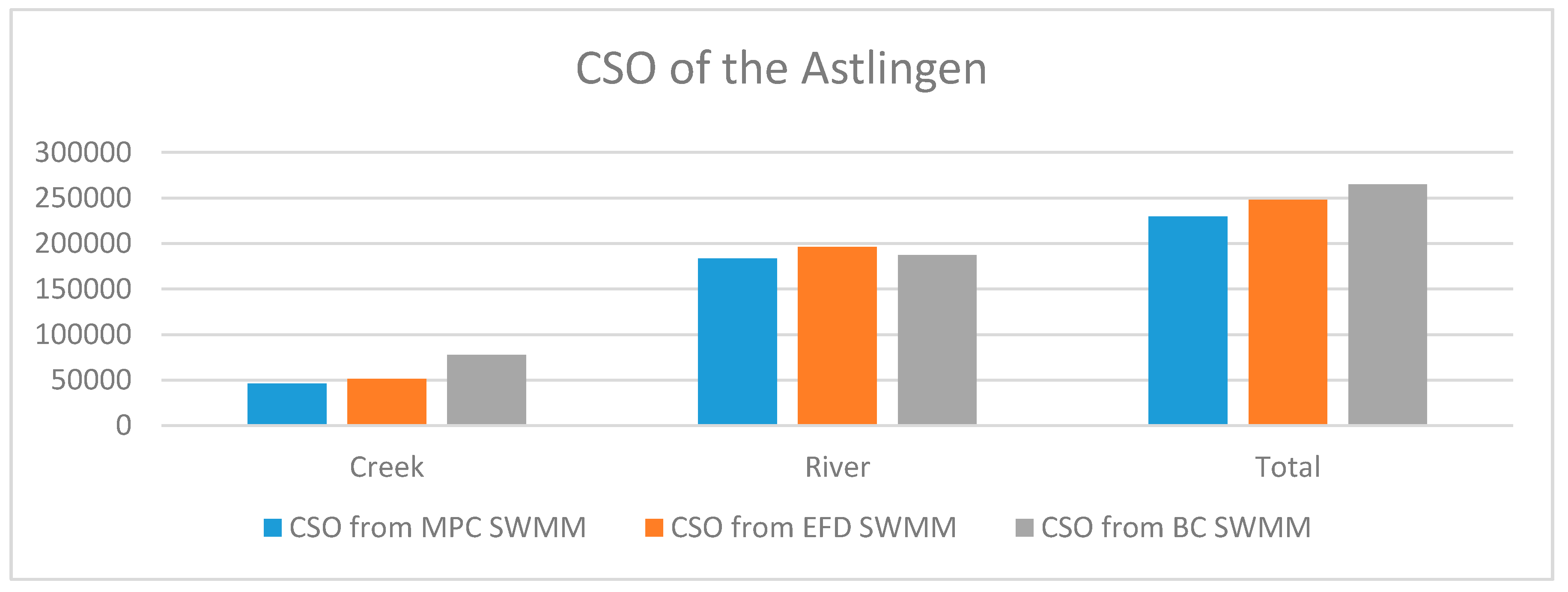
The simulated CSO volumes resulting from the application of MPC to the SWMM implementation of Astlingen are shown in

Table 6. Simulated CSO volumes (m³) for the Model Predictive Control (MPC) scenario, and percentage difference from the BC and Equal-Filling Degree Verification (EFD) scenarios. Positive variations denote reductions in CSO volume, while negative values denote increases in discharges.

Tank & CSO	MPC (m3)	EFD (%)	BC (%)
Tank 1	93251	6.49	−17.36
Tank 2	15484	37.77	52.90
Tank 3	34017	−29.69	−23.25
Tank 4	4814	48.55	56.85
Tank 5	15147	2.02	2.02
Tank 6	37950	12.86	45.47
CSO 7	4016	−1.11	−1.11
CSO 8	16207	−1.91	−1.92
CSO 9	4030	−1.46	−1.46
CSO 10	4838	−1.83	−2.05
River	183754	6.39	1.84
Creek	45996	10.68	40.68
Total	229750	7.28%	13.21%

, along with the percentage volume reduction compared to volumes for the BC and EFD scenarios. Compared to the BC and EFD scenarios, the MPC discharged significant less CSO volumes to the river and creek for most of the storage tanks (up to over 50% reduction for single discharge points). Considering that the MPC scenario led to an increase of discharges from some CSO structures, the overall improvement was around 7% and 13% against EFD and BC, respectively. It can be seen that the discharges from the passive parts of the system (CSO7-10, Tank1 and 5) increased with around 1%–2% as a result of control choices and due to backwater flows. The MPC successfully managed to achieve a major CSO reduction for the most sensitive part of the system (creek). These results are further illustrated by Figure 4, where the CSO volumes are subdivided according to the receiving water body.

4.2.2. CSO Events

The simulated number of CSO events and days with recorded CSOs for the MPC scenario are shown in

Table 7. Simulated CSO events for the MPC, EFD, and BC scenarios.

CSO Events	MPC	EFD	BC
Number	58	58	61
Days	70	65	62

, together with results from the BC and EFD scenarios. Since some CSO events took place over midnight, there was a discrepancy between these two values. Overall, the MPC and EFD scenarios produced less CSO events, but more days with CSOs than in the BC scenario. This suggests that both the control strategies stored water in the system more efficiently, and that they caused longer (but smaller) CSO events. Also, coupled rain events can be lumped into a single event due to the increased storage and longer emptying of the tanks. Indeed, CSO events were defined based on the physical characteristics of the system, i.e., a six-hour threshold was used to distinguish them. Considering that the total storage volume in the system was 5900 m³ and that the system can be emptied with a maximal rate of 0.271 m³/s [5], it took roughly six hours to empty the system in the BC scenario. This emptying time was clearly increased by the control algorithms in the EFD and MPC scenarios.

5. Conclusions

This paper presents a hydrodynamic model of the Astlingen benchmark network in the open-source software SWMM, enabling a more widespread usage of Astlingen for benchmarking complex control strategies. The development of this detailed model provides a unified test-bed, which allows the interested researchers and engineers to use and compare performance of different control methodologies. This will also solve practical difficulties confronted by researchers or interested engineers to share models and data of real-life urban drainage systems for RTC implementations.

The detailed hydrodynamic model was developed to emulate the reference the conceptual model using a three-step procedure and two model development criteria. The performance of the SWMM model was evaluated against the reference model by comparing a local throttle control (Base Case) and a global RTC approach (EFD rule-based strategy). The developed model and data are freely available on a public repository and they can be downloaded and applied directly through EPA-SWMM with different RTC approaches configured by interested practitioners.

The potential of the detailed SWMM model of the Astlingen benchmark network for testing complex control algorithms was demonstrated by applying an MPC strategy. This was described with clear internal model and core principle definitions. The MPC utilizes the conceptual model of Astlingen to generate optimal control actions, while the detailed SWMM model was used for the fine-tuning of the control setpoints. In order to integrate the optimization and simulation processes, a closed-loop scheme of MPC and SWMM was used. This configuration can be used in other cases other than Astlingen, and with any other complex control algorithm (RTC and MPC).

The flexibility of the proposed implementation of the Astlingen benchmark model was shown for different control strategies, with different level of complexity, ranging from simple local controls (BC), global RTC (EFD), and complex MPC strategies. Researchers and practitioners therefore now have a new useful case for testing and comparing different control strategies.

References

- Schütze, M.; Campisano, A.; Colas, H.; Schilling, W.; Vanrolleghem, P. Real time control of urban wastewater systems—Where do we stand today? J. Hydrol. 2004, 299, 335–348. [Google Scholar] [CrossRef]
- García, L.; Barreiro-Gomez, J.; Escobar, E.; Téllez, D.; Quijano, N.; Ocampo-Martinez, C. Modeling and real-time control of urban drainage systems: A review. Adv. Water Resour. 2015, 85, 120–132. [Google Scholar] [CrossRef] [Green Version]
- Sun, C.C.; Cembrano, G.; Puig, V.; Meseguer, J. Cyber-physical systems for real-time management in the urban water cycle. In Proceedings of the 4th International Workshop on Cyber-Physical Systems for Smart Water Networks, Porto, Portugal, 10–13 April 2018; pp. 5–8. [Google Scholar]
- Cembrano, G.; Quevedo, J.; Salamero, M.; Puig, V.; Figueras, J.; Martí, J. Optimal control of urban drainage systems. A case study. J. Contr. Engin. Pract. 2004, 12, 1–9. [Google Scholar] [CrossRef]
- Schütze, M.; Lange, M.; Pabst, M.; Haas, U. Astlingen—A benchmark for real time control (RTC). Water Sci. Technol. 2017, 2, 552–560. [Google Scholar] [CrossRef] [PubMed]
- DWA 2005 Framework for Planning of Real Time Control of Sewer Networks. Guideline DWA-M 180E, German Association for Water, Wastewater and Waste, DWA, December 2005. Available online: https://webshop.dwa.de/de/guideline-dwa-m-180-december-2005.html (accessed on 1 October 2019).
- Meneses, E.J.; Gaussens, M.; Jakobsen, C.; Mikkelsen, P.S.; Grum, M.; Vezzaro, L. Coordinating rule-based and system-wide model predictive control strategies to reduce storage expansion of combined urban drainage systems: The case study of Lundtofte, Denmark. Water 2018, 20, 76. [Google Scholar] [CrossRef] [Green Version]
- Klepiszewski, K.; Schmitt, T. Comparison of conventional rule based flow control with control processes based on fuzzy logic in a combined sewer system. Water Sci. Technol. 2002, 46, 77–84. [Google Scholar] [CrossRef] [PubMed]
- Sun, C.C.; Joseph, B.; Maruejouls, T.; Cembrano, G.; Muñoz, E.; Meseguer, J.; Montserrat, A.; Sampe, S.; Puig, V.; Litrico, X. Efficient integrated model predictive control of urban drainage systems using simplified conceptual quality models. In Proceedings of the 14th IWA/IAHR International Conference on Urban Drainage, Prague, Czech Republic, 10–15 September 2017; pp. 1848–1855. [Google Scholar]
- Sun, C.C.; Joseph, B.; Cembrano, G.; Puig, V.; Meseguer, J. Advanced integrated real-time control of combined urban drainage systems using MPC: Badalona case study. In Proceedings of the 13th International Conference on Hydroinformatics, Palermo, Italy, 1–5 July 2018; pp. 2033–2041. [Google Scholar]
- Lund, N.S.V.; Falk, A.K.V.; Borup, M.; Madsen, H.; Mikkelsen, P.S. Model predictive control of urban drainage systems: A review and perspective towards smart real-time water management. Crit. Rev. Environ. Sci. Technol. 2018, 48, 279–339. [Google Scholar] [CrossRef]
- Borsanyi, P.; Benedetti, L.; Dirckx, G.; De Keyser, W.; Muschalla, D.; Solvi, A.M.; Vandenberghe, V.; Weyand, M.; Vanrolleghem, P.A. Modelling real-time control options on virtual sewer systems. J. Environ. Eng. Sci. 2008, 7, 395–410. [Google Scholar] [CrossRef]
- 10ifak 2018: Simba# 3.0—Manual, ifak Institute for Automation and Communication, Magdeburg, 39106, Germany, 2018. Available online: https://nextcloud.ifak.eu/s/simba3?path=%2FFlyer#pdfviewer (accessed on 1 October 2019).
- Sun, C.C.; Joseph, B.; Maruejouls, T.; Cembrano, G.; Meseguer, J.; Puig, V.; Litrico, X. Real-time control-oriented quality modelling in combined urban drainage networks. In Proceedings of the 20th IFAC World Congress, Toulouse, France, 9–14 July 2017; pp. 3941–3946. [Google Scholar]
- Sun, C.C.; Joseph, B.; Maruejouls, T.; Cembrano, G.; Muñoz, E.; Meseguer, J.; Montserrat, A.; Sampe, S.; Puig, V.; Litrico, X. Conceptual quality modelling and integrated control of combined urban drainage system. In Proceedings of the 12th IWA Conference on Instrumentation, Control and Automation, Quebec City, Canada, 11–16 June 2017; pp. 141–148. [Google Scholar]
- Fu, G.; Khu, S.; Butler, D. Optimal distribution and control of storage tank to mitigate the impact of new developments on receiving water quality. J. Environ. Engine. 2010, 136, 335–342. [Google Scholar] [CrossRef]
- Sun, C.C.; Puig, V.; Cembrano, G. Real-Time Control of Urban Water Cycle under Cyber-Physical Systems Framework. Water 2020, 12, 406. [Google Scholar] [CrossRef] [Green Version]
- Rossman, L. Storm Water Management Model Users’ Manual Version 5.1; Environmental Protection Agency: Washington, DC, USA, 2015.
- DWA 2018 Abflusssteuerung in Kanalnetzen—Anwendungsbeispiel. DWA-Themenband T1/2018, German Association for Water, Wastewater and Waste, DWA, November 2018. Available online: https://www.ifak.eu/de/bibcite/reference/5042 (accessed on 1 October 2019).
- Müller, T.; Schütze, M.; Bárdossy, A. Temporal asymmetry in precipitation time series and its influence on flow simulations in combined sewer systems. Adv. Water Resour. 2017, 107, 56–64. [Google Scholar] [CrossRef]
- Rossman, L.A.; Huber, W.C. Storm Water Management Model Reference Manual Volume 1—Hydrology, EPA, www2.epa.gov/water-research, January 2016. Available online: https://cfpub.epa.gov/si/si_public_record_report.cfm?Lab=NRMRL&dirEntryId=309346 (accessed on 1 October 2019).
- Nash, J.E.; Sutcliffe, J.V. River flow forecasting through conceptual models part I-A discussion of principles. J. Hydrol. 1970, 10, 282–290. [Google Scholar] [CrossRef]
- Halvgaard, R.; Falk, A.K.V. Water system overflow modelling for model predictive control. In Proceedings of the 12th IWA Specialized Conference on Instrumentation, Control and Automation, Quebec City, Canada, 11–16 June 2017; pp. 1–4. [Google Scholar]
- Dirckx, G.; Van Assel, J.; Weemaes, M. Real Time Control from Desk Study to Full Implementation. In Proceedings of the 13th International Conference on Urban Drainage, Kuching, Malaysia, 7–12 September 2014. [Google Scholar]
- Singh, V.P. Hydrologic Systems. Volume 1: Rainfall-Runoff Modelling; Prentice Hall: Bergen, NJ, USA, 1988. [Google Scholar]
- Maciejowski, J.M. Predictive Control: With Constraints; Prentice Hall: Bergen, NJ, USA, 2002. [Google Scholar]
- Svensen, J.L.; Niemann, H.H.; Poulsen, N.K. Model Predictive Control of overflow in sewer networks. In Proceedings of the 4th International Conference on Control and Fault-tolerant Systems, Casablanca, Morocco, 18–20 September 2019. [Google Scholar]
Figure 1.
Scheme of Astlingen Sewer Network (adapted from [5]), showing the location of the 10 subcatchments (SC) and combined sewer overflow (CSO) structures, along with the six basins (with respective storage volumes). Transport times are long the network are expressed in minutes.
Figure 2.
The closed-loop Real-Time Control (RTC) scheme.
Figure 3.
Layout of the detailed SWMM model of Astlingen benchmark network.
Figure 4.
Comparison of CSO volumes for the MPC, EFD, and BC scenarios subdivided by the receiving water body.