Investigating the Impacts of Water Conservation on Water Quality in Distribution Networks Using an Advection-Dispersion Transport Model

1
Department of Civil and Materials Engineering, The University of Illinois at Chicago, Chicago, IL 60607, USA
2
Department of Civil, Architectural and Environmental Engineering, The University of Texas at Austin, Austin, TX 78712, USA
*
Author to whom correspondence should be addressed.
Water 2020, 12(4), 1033; https://doi.org/10.3390/w12041033
Submission received: 8 March 2020
/
Revised: 28 March 2020
/
Accepted: 31 March 2020
/
Published: 4 April 2020
(This article belongs to the Special Issue Multi-Quality Water Distribution Systems Analysis: Simulation and Management)
Abstract
:With the increasing adoption of demand management strategies and water conservation practices, domestic water consumption is projected to decline in the future. The subsequent consumer-side demand reductions are expected to result in increased residence times in water distribution networks (WDNs), and thus could have negative effects on the water quality (WQ) reaching the consumers’ taps. This study evaluates the impacts of the projected decrease in residential water demands on the deterioration of the WQ in WDNs. This deterioration will likely be most prominent in the dead-end branches at the perimeters of WDNs, where the flow is characteristically low and intermittent. The assessment of WQ deterioration in the dead-end branches requires the implementation of an accurate WQ simulation model. To this end, a new Python-based software package, WUDESIM_Py, is first introduced. The WQ simulation engine in WUDESIM_Py is based on an advection-dispersion-reaction model and accounts for the spatial distribution of water demands along dead-end pipes. WUDESIM_Py comprises various sets of functions that allow the users to set-up and conduct WQ simulations as well as obtain and visualize simulation results. A complete description of the different functions, together with examples of how these functions can be implemented in different applications, is provided. Through conducting extensive simulations of benchmark WDNs, the results revealed that widespread adoption of water conservation practices can lead to significant WQ deterioration in the dead-end branches. Additionally, the results suggested that neglecting dispersive transport and spatially aggregating demands may result in overestimating residual chlorine concentrations in the dead-end branches, which could mask the real impacts of demand reduction on WQ deterioration.
1. Introduction
Soon after EPANET (EPANET is a public domain, water distribution system modeling software package developed by the United States Environmental Protection Agency’s Water Supply and Water Resources Division) [1] came to light in the early-1990s, it quickly became the primary go-to software for hydraulic and water quality (WQ) analysis of water distribution networks (WDNs). The widespread implementation of EPANET by both engineering practitioners and researchers could be credited to its public-domain license and the fact that it is distributed/endorsed by the US Environmental Protection Agency (EPA) [2]. EPANET’s hydraulic simulation engine allows running extended period simulations of WDN hydraulics, while its WQ engine allows modeling single-species reactions in the bulk flow and at the pipe wall [3]. The graphical user interface (GUI) of EPANET enables the users to build and edit WDN models, conduct simulations, and obtain/visualize simulation results. Additionally, users could access individual functions inside EPANET using the dynamic link library (DLL) programmers’ toolkit [4]. To date, EPANET has been used in numerous research studies that leveraged its hydraulic and WQ analysis capabilities into optimizing the design and operation of WDNs [5] and supporting the security and resilience of WDNs in the face of natural and man-made hazards [6].
Alongside the abovementioned research efforts, copious attempts have been made over the years to develop software in order to increase the usability, and extend the capabilities, of EPANET. These efforts could be broadly classified into: (1) Modifications to, and/or extensions of EPANET’s engine, and (2) wrapper packages built upon EPNAET’s DLL, usually in other programming languages. Wrapper packages are typically limited to providing the users with easy access to the different DLL functions and enabling them to readily retrieve, analyze, and visualize simulation results. Engine modifications/extensions go beyond that by either enhancing the modeling and simulation capabilities of EPANET, or by adding new capabilities, such as threat detection and risk assessment. Notable examples of engine modifications/extensions include adding the capability to simulate multi-species in EPANET-MSX [7], incomplete mixing at junctions in EPANET-BAM [8], and AZRED [9], pressure-dependent hydraulics in EPANET-PDX [10] and EPANET-PMX [11], cyber-physical attack analysis in EPANETcpa [12], and sensor placement optimization in TEVA-SPOT [13]. In addition, wrapper packages were written in different programming languages, including Python, Matlab, R, GNU Octave, C#, and JavaScript. Table 1 gives a non-exhaustive list of the important engine extensions and wrapper packages that have appeared in recent literature with a brief description of the added capabilities.
Despite its wide implementation, EPANET’s WQ engine encompasses a number of limitations that originated from some of the fundamental assumptions associated with its development [31]. One of these assumptions is that the transport of various species in the pipes of WDNs is solely driven by advective flow [3]. Hence, the outspread of species along the pipes by longitudinal dispersion is neglected. While this assumption is somewhat valid for main transmission lines that convey large quantities of water and consistently operate under turbulent conditions, it was found to yield significant simulation errors for low-flow pipes at the perimeters of WDNs. Numerous studies have demonstrated the importance of including solute transport by dispersion, particularly in the low-flow pipes (see, for example, [32,33,34,35,36,37] and references therein). Additionally, spatial demand aggregation that typically arises from WDN skeletonization magnifies these errors, thus leading to substantial discrepancies between simulated and field-measured concentration profiles [38].
Recent studies have demonstrated that simulation errors caused by ignoring dispersive transport and demand aggregation are most evident in the dead-end branches (DEBs) of WDNs, where the flow is intermittent and mostly within the laminar regime [38]. Furthermore, DEBs are more vulnerable to WQ monitoring violations, which makes them hotspots for WQ deterioration [39,40]. In a recent effort, Abokifa et al. released WUDESIM [17], a public-domain C/C++ software toolkit for simulating single-species WQ in the DEBs of WDNs. In addition to advective transport, WUDESIM includes species transport by longitudinal dispersion, and corrects for simulation errors that arise from spatial demand aggregation along the DEB pipes [38]. Accounting for dispersive transport and spatial demand distribution along the pipes was shown to enhance the simulation accuracy compared to EPANET [38], and to yield more reliable outcomes for WQ optimization [41].
With the forecasted decline in domestic water consumption under the increasing adoption of water conservation and demand management practices, flow rates in WDNs are projected to decrease in the future. In 2017, approximately 68% of water utilities in the US reported sponsoring active water conservation programs. Such programs are largely focused on consumer-side demand management using a variety of incentives and technological solutions. Hence, reductions in consumer-side demands will likely increase residence times, and in turn water ages in WDNs, which may lead to further deterioration of the WQ [42]. Water quality deterioration will likely be most pronounced in the problematic DEBs of WDNs, where the flow is characteristically low and intermittent. In a recent study, Zhuang and Sela [43] investigated the effects of changes in residential demand profiles on WDN performance in response to emerging demand management strategies. Their results revealed a significant decrease in the water age for eight tested WDN models. However, their study relied on the water age as the sole indicator of the WQ, and hence did not fully capture the influence of demand reduction on more significant WQ parameters. For instance, disinfectant residuals are routinely monitored by water utilities for regulatory compliance purposes, and their concentrations in WDNs are dictated by flow-driven reactive-transport.
Building upon the previous studies, the objectives of this paper are to (1) contribute to the current efforts by the WDN analysis community to provide software that augments the capabilities of EPANET’s WQ simulation engine and enhance its usability, and (2) to investigate the impact of water conservation strategies on the WQ in WDNs using an advanced WQ simulation model. To this end, WUDESIM_Py, an open-source Python-based extension for simulating advection-dispersion reactive-transport of single-species in WDNs is first introduced. WUDESIM_Py is freely available in the Python Package Index (PyPI) and comprises various sets of functions that: (1) Enable the users to readily set-up and run WQ simulations in both EPANET and WUDESIM; (2) provide the users with easy access to all the internal functions of the WUDESIM C/C++ toolkit; and (3) visualize and analyze the results of WQ simulations of DEBs. Second, WUDESIM_Py is applied to assess the effects of demand reduction on disinfectant concentrations in WDNs, with a focus on the problematic DEBs. Accordingly, extensive simulations of various WDN models are conducted, and the degradation in the integrity of the WQ under demand reduction strategies is assessed by means of representative performance metrics.
2. Materials and Methods
2.1. WUDESIM_Py Software Package Description
The WUDESIM_Py package is a set of Python commands that are built to wrap the WUDESIM C/C++ DLL toolkit [17] and enable the users to run single-species WQ simulations of the DEBs of WDNs using both advection and dispersion transport mechanisms. Additionally, it implements corrections for the simulation errors that originate from spatial demand aggregation and allows the users to stochastically generate demands at fine time scales to use in the WQ simulations. A complete description of the underlying advection-dispersion transport model can be found in reference [17].
As a wrapper package, WUDESIM_Py provides the users with access to all the individual C/C++ functions that run the analysis and write the output/report files without requiring the explicit use of additional packages to call functions and convert data types across different programming languages (e.g., ctypes). In addition to wrapping the toolkit functions, WUDESIM_Py comprises additional functions for retrieving, analyzing, and visualizing the simulation results. The functions in WUDESIM_Py are specifically designed for users familiar with the EPANET programmers’ toolkit environment and the overlying wrapper packages that were introduced in the literature (Table 1).
In the following sections, the procedure of running a simulation in WUDESIM_Py is first explained, followed by a brief description of the different functions in WUDESIM_Py and examples (i.e., code snippets) of how the users can implement the package in specific applications. Python scripts of the software package, example scripts provided herein, and scripts used to conduct all the analyses in this study are available on Github at (https://github.com/aabokifa/WUDESIM_Py).
2.1.1. Simulation Procedure
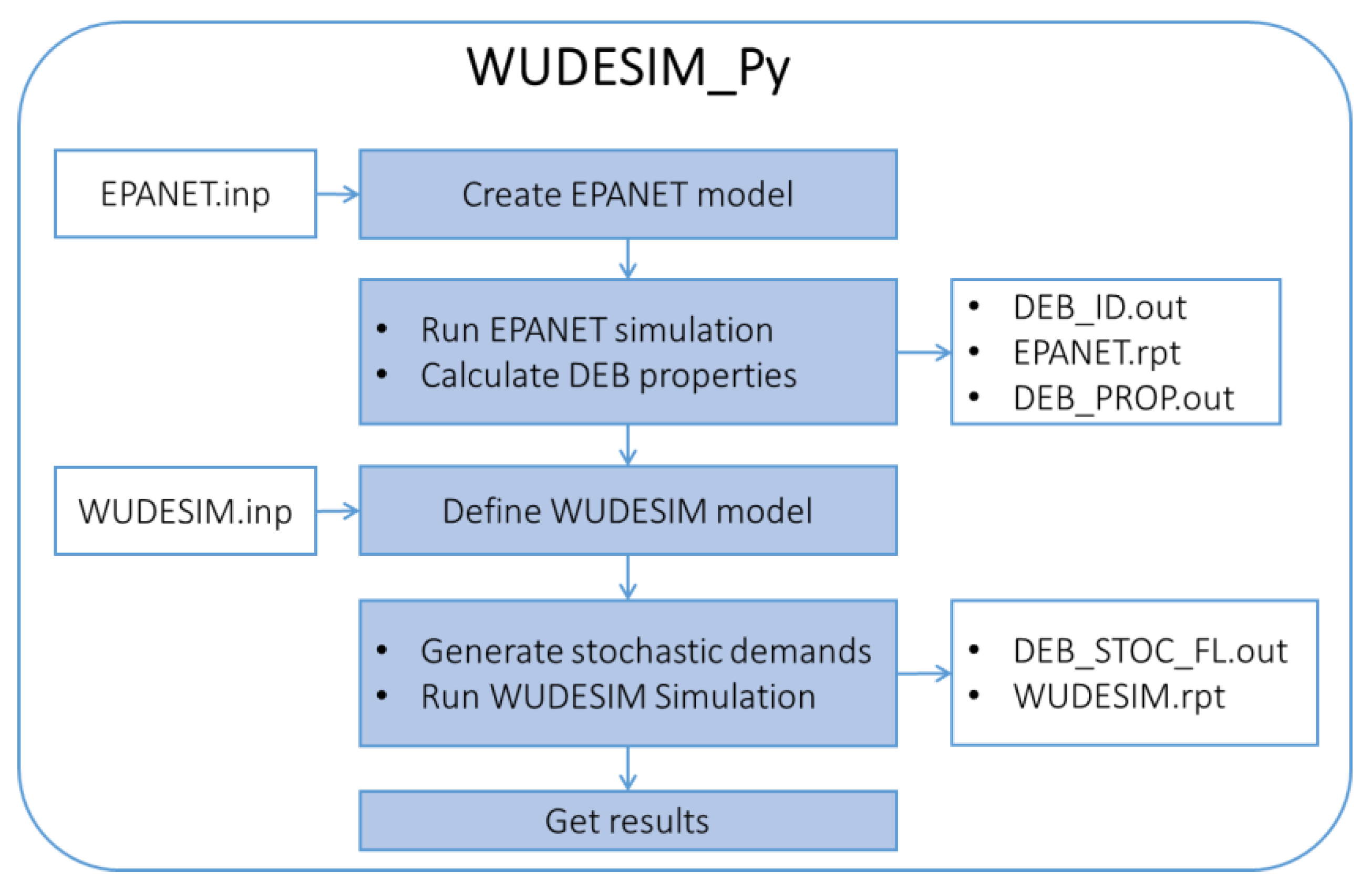
The overall procedure of running a simulation using WUDESIM_Py is depicted in Figure 1, and proceeds as follows:
- The EPANET input (.inp) file is first read to create the network model and obtain all the network parameters.
- WUDESIM_Py then discovers all the DEBs in the WDN, runs a full hydraulic and WQ simulation using EPANET, and calculates the average properties of the DEBs in the network. EPANET simulation results are written to the EPANET report (.rpt) file, and the IDs and properties of DEBs are written to output files “DEB_ID.out” and “DEB_PROP.out”, respectively.
- The WUDESIM input (.inp) file is then read to define the WUDESIM model parameters for calculating dispersion coefficients, demand aggregation corrections, and stochastic demands. The user can choose to simulate either all or a subset of the DEBs using WUDESIM.
- WUDESIM_Py runs a WQ simulation for the selected DEBs and writes the results to the WUDESIM report (.rpt) file. If selected by the user, stochastic demands are generated and used in the simulation, and the generated flow profiles are written to “DEB_STOC_FL.out”.
- WUDESIM_Py allows the users to retrieve and/or visualize the results at any stage during the simulation procedure.
2.1.2. Functions and Capabilities
The WUDESIM_Py software package has 9 different sets/families of functions. Each set provides different capabilities and functionalities, including setting up and running the simulations, writing the results to output files, obtaining the properties of the network, and retrieving and visualizing simulation results. Below, a list of the different families of functions in WUDESIM_Py, together with a brief description of their capabilities is provided.
- Engine Functions: These functions (Table 2) allow the users to start a new project, find DEBs in a WDN, run WQ simulations, calculate average properties, and generate stochastic demands.
- Get Index/ID Functions: These functions (Table 3) allow the users to obtain the index of any dead-end branch, pipe or node in the WDN given its ID and vice versa.
- Get Property Functions: These functions (Table 4) retrieve the values of different network properties, including the number of DEBs, the number of simulation steps, the size of a given DEB, and the dimensions of a DEB pipe.
- Get Result Functions: These functions (Table 5) retrieve the value of the simulation results for a specific pipe or node at a specific time step (i.e., a single value). Pipe results include the Reynolds and Peclet numbers, residence time, and flow rate, while node results include WQ and demand.
- Get All IDs Functions: These functions (Table 6) enable the users to obtain lists of the IDs of all DEBs, pipes, and nodes in the WDNs.
- Get All Properties Functions: These functions (Table 7) allow the users to obtain Pandas data frames (DFs) with all the properties of all dead-end branches, pipes, and nodes based on EPANET simulation. Branch properties include the size, total length, and total residence time, while pipe properties include length, diameter, mean Reynolds, mean flow rate, and mean residence time. Node properties include mean WQ and mean demand.
- Get Time Series Functions: These functions (Table 8) allow the users to retrieve DFs with the time series (TS) simulation results for a specific pipe or node. Pipe results include the Reynolds and Peclet numbers, residence time, and flow rate, while node results include WQ and demand.
- Visualize Functions: These functions (Table 9) allow the users to plot the WDN layout highlighting specific DEB pipes or nodes or plot the TS results for a specific pipe or node.
- Writing Functions: These functions (Table 10) enable the users to generate individual output and report files containing WDN properties, simulation results, and stochastic demands.
In addition to the aforementioned families of functions, WUDESIM_Py includes a master function, RUN_FULL_SIM, which takes the names of the EPANET and WUDESIM input (.inp) and report (.rpt) files and conducts a complete simulation as well as generate all the output/report files as shown in Figure 1. Depending on their needs, the users can readily use this master function to conduct a complete analysis instead of having to call each of the ENGINE and WRITE functions individually.
2.1.3. Code Examples
This section provides example code snippets of the implementation of the various functions in WUDESIM_Py for different scenarios.
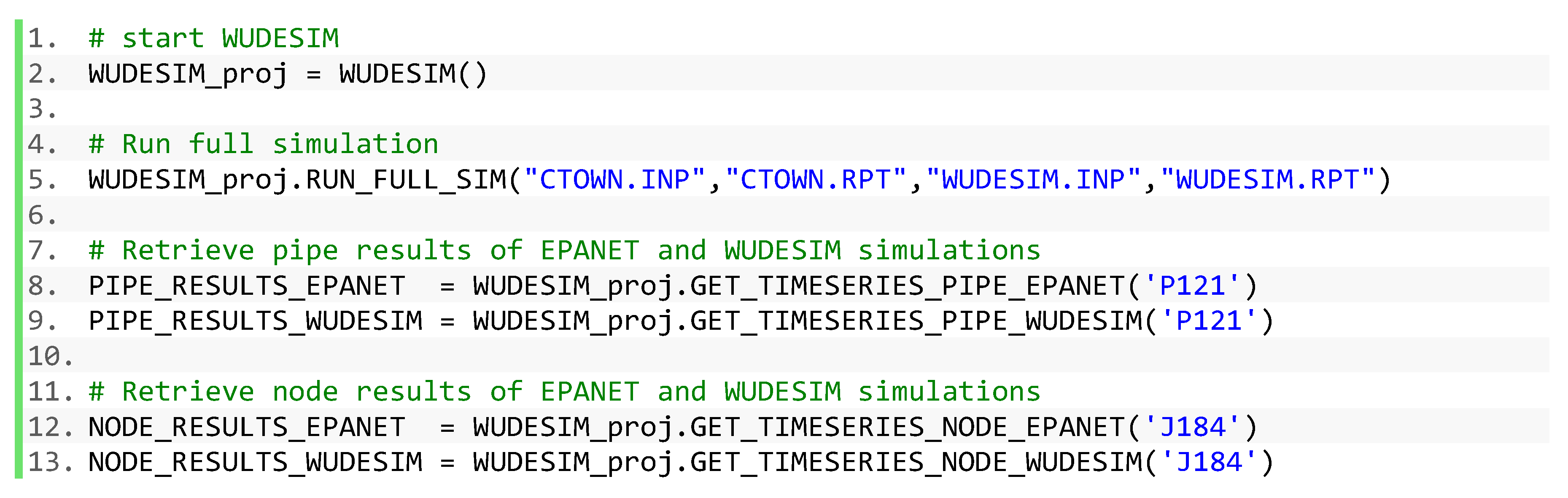
• Example 1—Running a full simulation:
In this example, the user is interested in conducting a full simulation and retrieving the EPANET and WUDESIM simulation results of a specific pipe and node. As shown in the code snippet depicted in Figure 2, a new instance of WUDESIM is first created, and then the RUN_FULL_SIM function is called with the names of the input and output files of both EPNET and WUDESIM. Then, the GET_TIMESERIES family of functions is called to retrieve the time-series simulation results for node (J184) and pipe (P121).
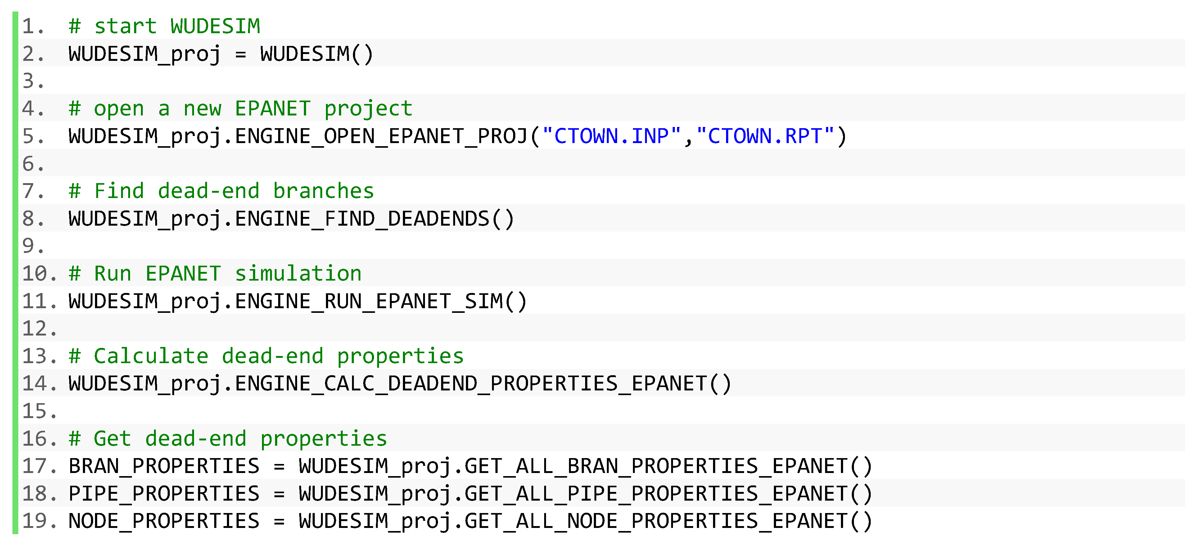
• Example 2—Getting the properties of DEBs:
In this example, the user is interested in identifying all the DEBs in the network and obtaining their average results based on an EPANET simulation. This could be useful in cases where the network model is large, and hence using WUDESIM to simulate all pipes will be computationally expensive. As shown in the code snippet depicted in Figure 3, a new instance of WUDESIM is first created, and then the series of ENGINE functions are called to open a new EPANET project, find the DEBs in the network, run the EPANET simulation, and calculate the average properties the DEBs based on the simulation results. Then, the GET_ALL family of functions is used to obtain data frames with all the properties of all dead-end branches, pipes, and nodes in the network.
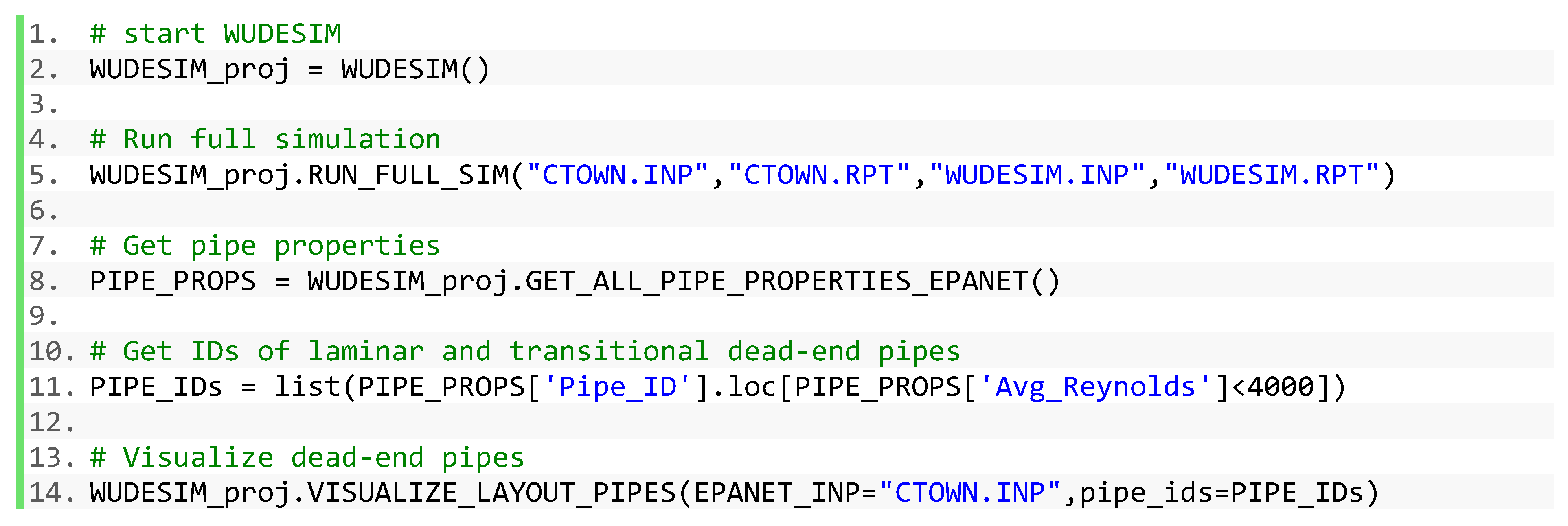
• Example 3—Visualizing the layout of DEBs:
In this example, the user is interested in visualizing all the dead-end pipes in the network with an average Reynolds number below 4000 (i.e., laminar and transitional flow pipes). As shown in the code snippet depicted in Figure 4, a new WUDESIM instance is first created, and a full simulation is conducted using the RUN_FULL_SIM function. The GET_ALL_PIPE_PROPERTIES function is used to retrieve the average properties of all dead-end pipes. Finally, the IDs of the pipes with an average Reynolds number below 4000 are extracted into a new list, which is passed into the VISUALIZE_LAYOUT_PIPES function for plotting. The same procedure can be used to visualize the layout of the nodes that have an average WQ below a certain threshold (e.g., chlorine concentrations below 0.2 mg/L).
2.2. Investigating the Impacts of Demand Reduction
Various conservation strategies, including upgrading to more water-efficient fixtures, installing smart meters that provide feedback about water usage, identifying opportunities for demand reduction, as well as augmenting water supply for non-potable uses through rainwater harvesting, have all shown a strong potential to reduce residential consumption, which in some cases can reach up to 50% [44,45].
To investigate the impacts of demand reduction resulting from potential water conservation strategies on the WQ in WDNs, we relied on extensive simulations and performance metrics, as described in the following sections. Specifically, our objective was twofold: (1) Assess the degradation in the integrity of the WQ with a projected decrease in residential water demands, and (2) evaluate the impact of implementing an advection-dispersion model on assessing WQ degradation due to demand reduction.
2.2.1. Demand Scenarios and Water Quality Simulations
To model the impact of conservation strategies, two demand scenarios were investigated: (1) Nominal demand scenario—representing the current residential demand, which varies throughout the day and peaks twice per day during the morning and late-evening hours; and (2) reduced demand scenario—representing the response to conservation efforts in which the overall demand supplied by the WDN is uniformly reduced by 50% (i.e., the total daily demand is 50% that of the nominal demand scenario). The two demand scenarios were implemented by modifying the demand patterns assigned to the consumption nodes in the hydraulic simulations, as explained in more detail in the results section.
WUDESIM_Py was used to conduct WQ simulations under both scenarios in order to evaluate the impacts of demand reduction on chlorine residual concentrations in the dead-end branches. The simulations were conducted in both EPANET and WUDESIM, and the results from both models were compared to assess the influence of using an advanced model on the simulated WQ deterioration.
2.2.2. Performance Metrics
To evaluate the performance of a given WDN under the two demand scenarios, 3 metrics, namely reliability, resilience, and vulnerability (RRV) [46,47], were calculated based on the simulations conducted using both EPANET and WUDESIM. RRV metrics represent a comprehensive measurement of the probability of success or failure of a system, its ability to recover from failure, and the consequences of a failure, respectively. Failure was defined here as the event in which the chlorine concentration at a specific location (i.e., a dead-end node) in the WDN was less than some predefined threshold.
The RRV performance metrics were calculated based on the simulation results during a certain evaluation period. To explain how the RRV metrics were calculated, the simulated chlorine concentrations during the evaluation period at each dead-end node was represented by a time series: , where is the total number of time steps and is the number of dead-end nodes in the WDN. To compute the reliability index, the state indicator () was first evaluated to identify success and failure events. For each dead-end node () at each timestep (), the value of was equal to 1 if the simulated chlorine concentration was greater than or equal the safety threshold (), and 0 otherwise:
Subsequently, the overall reliability of a dead-end node () is defined as the fraction of time during which chlorine concentration at node () is above the threshold:
The recovery metric () indicates whether the chlorine concentration recovers to normal (i.e., above the threshold) right after a violation (i.e., below the threshold) takes place:
Subsequently, the resilience index of a dead-end node () measures the number of occurrences when the concentration at a node recovers right after the threshold is violated over the number of violations:
Intuitively, reliability characterizes the frequency at which the chlorine residual requirement is satisfied, and resilience quantifies how quickly the system recovers from failure. Furthermore, the vulnerability of a dead-end node () is defined as the normalized average magnitude of failure at each dead-end node, which quantifies the extent of the concentration violation during failure events:
All 3 metrics defined above, , range between 0 and 1 for each dead-end node. The RRV for the entire system can then be calculated by taking different statistics across all dead-end nodes in the network, such as the average, worst case, and value at risk [48]. A high-performance WDN will be characterized by high reliability and resilience and low vulnerability metrics.
3. Results and Discussion
To systematically evaluate the impact of demand reduction and implementing different WQ models (i.e., EPANET and WUDESIM) on the levels of disinfectant residuals in the WDN, publicly available models of eight WDNs were tested [49]. All hydraulic and WQ settings, including pump operation rules, time steps, and reaction parameters, were set to the same values for the simulations conducted using both EPANET and WUDESIM. First-order rate constants for chlorine decay in the bulk phase and at the pipe wall were set to and , respectively. The simulation duration was set to 2 weeks (336 h) to allow WQ in the system to stabilize. For the same reason, the first 100 h of the simulation was not included in the evaluation period based on which the performance metrics were calculated. The hydraulic and WQ time steps were chosen to be 1 h and 5 min, respectively. Source concentration at all reservoirs was set to 4 mg/L. For WUDESIM simulations, a global segment length of 15 m, which is typical of the spacing between consecutive premises in suburban cul-de-sacs in the US [50], was selected to correct for the errors caused by spatial demand aggregation. The concentration threshold, , was set to 0.2 mg/L, which is the threshold typically used by water utilities in the US to ensure sufficient protection against microbial recontamination in WDNs [51].
3.1. Benchmark Network Analysis
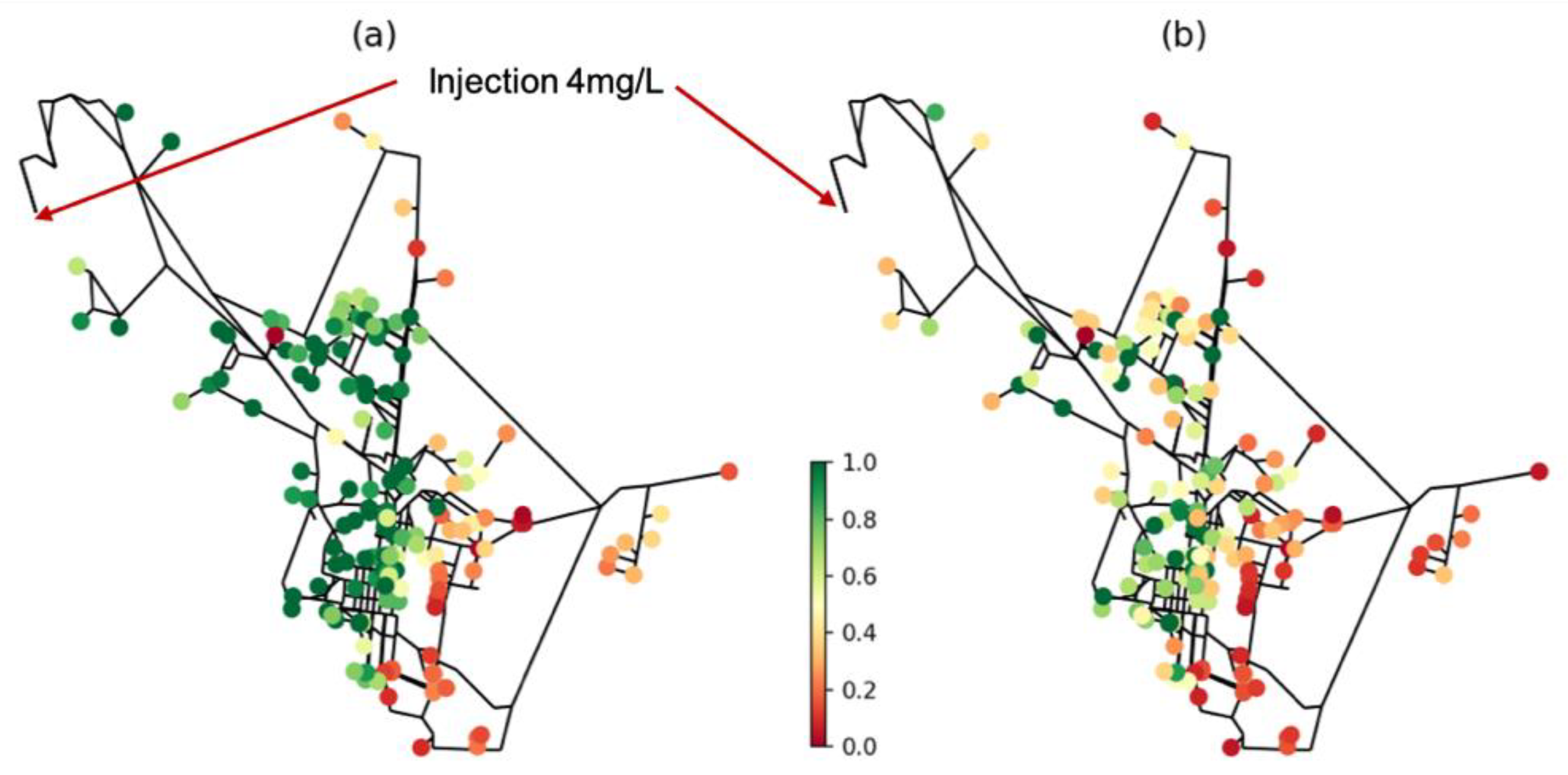
The results of WQ modeling using EPANET and WUDESIM, as well as the impact of demand reduction on network performance, were first demonstrated using a benchmark network, Net 6 [49]. Net 6, depicted in Figure 5, comprises 541 nodes, 642 pipes, 1 reservoir, 3 tanks, and 1 pump. In this benchmark network, 162 nodes were located in dead-end branches, making up approximately 30% of all network nodes. The network was supplied by a single reservoir with a chlorine concentration of 4 mg/L.
First, hydraulic and WQ simulations were performed under the nominal demand scenario. The hydraulic simulation in EPANET showed that 128 out of the 642 pipes were operating under laminar flow conditions, which indicates that the advection-reaction transport model embedded in EPANET was inappropriate for simulating these low-flow pipes. Instead, dispersive transport needs to be considered for these pipes to give accurate results since transport under laminar flow is dispersion-dominated. Hence, in addition to EPANET, WQ simulations were conducted in WUDESIM where solute dispersion was considered.
Chlorine residual concentrations at the dead-end nodes simulated by both EPANET and WUDESIM are shown in Figure 5a and Figure 5b, respectively, where the green markers represent high chlorine concentrations, and the red markers represent low concentrations. For EPANET simulation, 22 (14%) of the dead-end nodes had an average chlorine concentration below 0.2 mg/L, while in WUDEM simulation, 36 (22%) of the dead-end nodes had an average concentration below the threshold. The discrepancy in the simulation results indicates that EPANET overestimates chlorine concentrations at the dead-end nodes, thus yielding overly optimistic results when assessing the WQ compliance in WDNs.
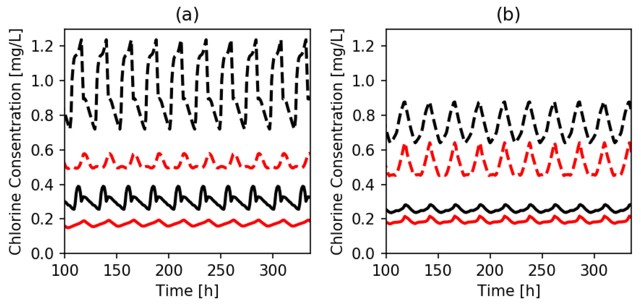
The overestimation in predicting chlorine concentrations by EPANET was further elucidated by comparing the concentration time-series during the evaluation period under both nominal and reduced demand scenarios. In Figure 6, black and red lines represent EPANET and WUDESIM simulation results, respectively, while dashed and solid lines symbolize the simulated concentrations under the nominal and reduced demand scenarios, respectively. Figure 6a illustrates the concentration profiles at an example dead-end node, J-169, while Figure 6b shows the average concentration profiles among all dead-end nodes during the evaluation period. It can be noticed from the figures that EPANET (black lines) overestimates the concentrations compared to WUDESIM (red lines) under both demand scenarios.
The overestimation of chlorine concentrations by EPANET is due to two reasons, namely neglecting dispersive transport and spatially aggregating water demands [38]. WUDESIM overcomes these errors by taking into account solute dispersion and correcting for the spatial distribution of flow demands along dead-end pipes [38]. Yet, it is crucial to note that in addition to considering a more advanced transport model, accurate simulation of disinfectant decay requires a more sophisticated reaction model than the simplistic first-order decay kinetics model that has been widely used in the literature [38]. Since chlorine is a highly reactive oxidant, it reacts with a variety of chemical and microbiological species as it transports through the pipes of the WDN. Hence, accurately accounting for the consumption of chlorine as a result of these parallel reactions would provide a better description of the decay kinetics, which was beyond the scope of this study.
As shown in Figure 6, chlorine concentrations in the dead-end nodes under reduced demand (solid lines) were significantly lower than those under nominal demand (dashed lines). The reduction percentage in chlorine concentration using both EPANET and WUDESIM was well above 60%. These results suggested that the potential risk of violation (i.e., chlorine residuals falling below the threshold) increased with the widespread implementation of water conservation and demand reduction practices. Thus, more attention should be paid to amending chlorine injection rates in order to account for the additional consumption in the WDN that takes place due to the increased residence time.
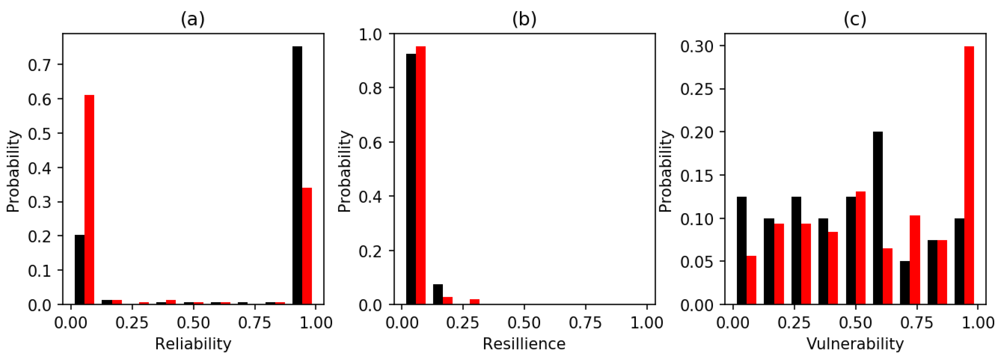
Since WUDESIM provides more accurate WQ predictions for the dead-end branches, it was utilized to evaluate the performance metrics under nominal and reduced demand scenarios in the subsequent analysis. Figure 7 shows the distributions of reliability, resilience, and vulnerability () of the nodes in Net6 under the nominal and the reduced demand scenarios (applied to all network nodes). Figure 7a demonstrates that under nominal demand, approximately 75% of the dead-end nodes exhibited reliability higher than 0.9, while 20% of the dead-end nodes had reliability lower than 0.1. This distribution implied that the dead-end nodes were considerably polarized in terms of reliability, where the chlorine concentration requirement was usually satisfied at 75% of the dead-end nodes and was rarely met at most of the remaining dead-end nodes. Moreover, when the demands were reduced, the portion of unreliable nodes increased significantly from 20% to 60%, while the reliable portion significantly decreased from 75% to 35%, thus resulting in a substantially less reliable system.
Figure 7b shows that the resilience of the benchmark network was rather low under both scenarios, which indicated that once a dead-end node failed to meet the chlorine concentration threshold, it typically remains in a failure state and rarely recovers. Under the reduced demand scenario, the resilience reaches a lower value compared to the nominal demand scenario, though the difference was not considerable. The vulnerability of dead-end nodes is shown in Figure 7c. Compared with the nominal demand scenario (black bars), the vulnerability of the reduced demand scenario (red bars) was relatively higher on the right-end and lower on the left end of the figure. This suggests that the magnitudes of violation instances were higher under the reduced demand scenario compared with the nominal demand scenario.
The average performance metrics for the benchmark network under both demand scenarios using EPANET and WUDESIM are summarized in Table 11. Taken together, the results showed that without proper adjustment of the chlorine dosage, demand reduction can exacerbate network performance in terms of chlorine residual by deteriorating reliability and resilience as well as increasing its vulnerability. Additionally, using EPANET WQ simulation model overestimates the WQ performance of the WDN.
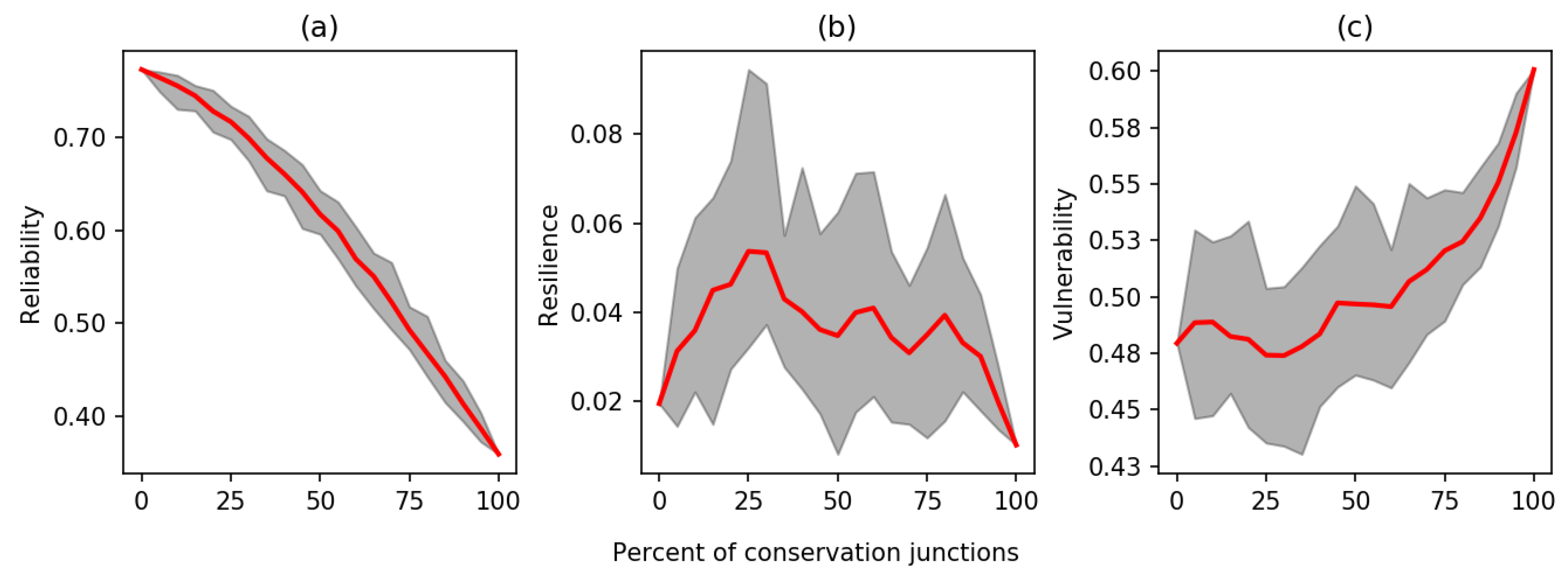
Previous analysis has demonstrated the deterioration of the WQ under the reduced demand scenario in which all nodes in the network adopt conservation strategies. Here, we evaluated the network response to the gradual adoption of the reduced demand, as shown in Figure 8 The response curve for each metric was attained by assigning conservation demand to a randomly selected set of nodes changing gradually from 0% to 100% of the total number of nodes in the network. To acquire representative samples of network responses, 30 random realizations were stimulated for each percentage of network users conforming to the reduced demand. In Figure 8, the red lines represent the average performance metrics of the 30 random realizations, and the shaded envelopes encompass the results from all 30 realizations. As expected, network reliability and vulnerability worsen as the number of consumer nodes experiencing reduced demand increases. Noticeably, the response curves were nonlinear with respect to the percentage of consumers with reduced demand. For example, the reduction in reliability (Figure 8a) and the increase in vulnerability (Figure 8c) were marginal when the percentage of the consumers with reduced demand increased from 0% to 25% compared to 75% to 100%. Interestingly, while reliability and vulnerability exhibited monotonic trends, the response of resilience to demand reduction was not monotonic, and the resilience scores remained low with very little variation. This observation could potentially suggest an intrinsic network property, indicating that targeted actions needed to be taken to recover chlorine residuals at dead-end nodes.
3.2. Global Analysis
The simulations and analyses conducted for the benchmark network were repeated herein for 7 additional WDNs to cover a wide range of network characteristics [49]. A summary of the network properties of all 8 WDNs simulated in this study is presented in Table 12, including the number of dead-end nodes and pipes operating under the laminar regime. The number of nodes in the networks ranged from 366 to 1614, while dead-end nodes accounted for 14% (Net 3) to 36% (Net 1) of the total nodes in the network. The EPANET simulation results suggested that under nominal demand, approximately 5% (Net 3) to 26% (Net 1) of the pipes had laminar flow; however, when operated under reduced demand, the number of pipes having laminar flow conditions increased to 9% for Net 3 up to 30% for Net 1. The differences in the number of dead-end nodes and laminar pipes reflected the difference in the topology of the networks, the magnitude of the user demands, and the operating rules of the network pumps.
The system performance metrics, i.e., RRV, of all the simulated networks under nominal and reduced demand scenarios using both EPANET and WUDESIM are summarized in Table 3. For Net 3 and Net 5, the reliability scores under the nominal demand scenario were 1, implying that all dead-end nodes satisfy the concentration threshold at all-time steps. Thus, the resilience and vulnerability scores, which are defined only for failure instances, have no entries in Table 3 for Net 3 and Net 5.
Additionally, Table 13 confirms the two observations made previously for the benchmark network. Firstly, under the same demand scenarios, WUDESIM predicts lower reliability and higher vulnerability than EPANET, indicating that EPANET overestimates the chlorine concentration at the dead-end nodes. Moreover, resilience scores, calculated based on EPANET and WUDESIM simulations, were low, which implies the inability of the dead-end nodes to recover after violating the chlorine residual requirement. Secondly, both EPANET and WUDESIM demonstrated a decrease in network performance, i.e., lower reliability and resilience, as well as high vulnerability, under reduced demands as compared to nominal demands. Overall, the results showed that reducing the demand across all tested WDNs caused a 5% to 42% decrease in network reliability, 0% to 9% decrease in resilience, and 5% to 33% increase in vulnerability. Taken together, these results revealed that the widespread adoption of water conservation practices could potentially pose a risk to public health due to the significant degradation of chlorine residuals, particularly in the dead-end branches.
4. Conclusions
Growing concerns over future water availability and safety are driving extensive water conservation efforts with the aim of reducing the pressure on public water supply systems. As new strategies and technologies are being increasingly implemented for promoting water conservation and reuse, a pressing need for assessing the adaptability of drinking water supply systems to changes in water demands arises. Hydraulic and water quality models are key to analyzing system performance, testing what-if scenarios, and estimating system response to changing conditions. Since design and planning decisions heavily rely on the outcomes of these models, their validity and accuracy are critical to ensure system integrity under different scenarios.
In this study, a newly developed open-source Python package, WUDESIM_Py, for simulating water quality in the low-flow dead-end branches of water distribution networks was introduced. WUDESIM_Py extends the water quality modeling capabilities of EPANET by implementing advection-dispersion reactive-transport of single-species and correcting for spatial demand aggregation along the dead-end pipes. WUDESIM_Py comprises many functions for running simulations, setting parameters, and retrieving and visualizing simulation results. Herein, a complete description of the various sets of functions in WUDESIM_Py, together with examples of how WUDESIM_Py can be employed for different applications, was first provided. Second, WUDESIM_Py was used to evaluate the impacts of demand reductions on the depletion of chlorine residuals in the dead-end branches of water distribution networks. The performance of the simulated networks under different scenarios was assessed through conducting extensive simulations of benchmark networks and using three performance measures for reliability, resilience, and vulnerability.
The results demonstrated that widespread adoption of water conservation practices may result in a significant deterioration in the water quality in the dead-end branches due to excessive degradation of chlorine residuals caused by the extended residence times. Additionally, the results suggested that neglecting dispersive transport and spatially aggregating demands may overestimate residual chlorine concentrations in the dead-end branches. More importantly, errors caused by neglecting dispersive transport and spatially aggregating demands were further exacerbated under reduced demand scenarios, which resulted in partially masking the deterioration in the water quality due to demand reduction. Taken together, the results of this study asserted that targeted actions need to be taken to recover chlorine residuals in the dead-end branches if water conservation practices are widely adopted.
Author Contributions
Conceptualization, A.A.A. and L.S.; methodology, A.A.A., L.X., and L.S.; software, A.A.A.; formal analysis, A.A.A. and L.X.; writing—original draft preparation, A.A.A. and L.X.; writing—review and editing, A.A.A. and L.S.; supervision, L.S.; project administration, L.S.; funding acquisition, L.S. All authors have read and agreed to the published version of the manuscript.
Funding
This research was funded by the University of Texas at Austin Startup Grant and by Cooperative Agreement No. 83595001 awarded by the U.S. Environmental Protection Agency (EPA) to The University of Texas at Austin. This work has not been formally reviewed by EPA. The views expressed in this document are solely those of the authors and do not necessarily reflect those of the Agency. EPA does not endorse any products or commercial services mentioned in this publication.
Conflicts of Interest
The authors declare no conflict of interest.
References
- Rossman, L.A. EPANET Users Manual, Version 1.1; Environmental Protection Agency: Cincinnati, OH, USA, 1994; pp. 1–122.
- Grayman, W.M. History of Water Quality Modeling in Distribution Systems. In Proceedings of the International WDSA/CCWI Joint Conference 2018, Kingston, ON, Canada, 23–25 July 2018. [Google Scholar]
- Rossman, L.A.; Clark, R.M.; Grayman, W.M. Modeling Chlorine Residuals In Drinking Water Distribution Systems. J. Environ. Eng. 1994, 120, 803–820. [Google Scholar] [CrossRef]
- Rossman, L. The EPANET programmer’s toolkit for analysis of water distribution systems. In Proceedings of the 29th Annual Water Resources Planning and Management Conference, Tempe, AZ, USA, 6–9 June 1999. [Google Scholar]
- Mala-Jetmarova, H.; Sultanova, N.; Savic, D. Lost in optimisation of water distribution systems? A literature review of system operation. Environ. Model. Softw. 2017, 93, 209–254. [Google Scholar] [CrossRef] [Green Version]
- Ostfeld, A. Enhancing water-distribution system security through modeling. J. Water Resour. Plan. Manag. 2006, 132, 209–210. [Google Scholar] [CrossRef]
- Shang, F.; Uber, J.G.; Rossman, L.A. Modeling reaction and transport of multiple species in water distribution systems. Environ. Sci. Technol. 2008, 42, 808–814. [Google Scholar] [CrossRef]
- Ho, C.K.; Khalsa, S.S. Epanet-Bam: Water Quality Modeling With Incomplete Mixing in Pipe Junctions. In Proceedings of the 10th Annual Water Distribution Systems Analysis Conference, Kruger National Park, South Africa, 17–20 June 2008; pp. 981–991. [Google Scholar]
- Choi, C.Y.; Shen, J.Y.; Austin, R.G. Development of a comprehensive solute mixing model (azred) for double-tee, cross and wye junctions. In Proceedings of the 10th Annual Water Distribution Systems Analysis Conference, Kruger National Park, South Africa, 17–20 June 2008; pp. 1004–1014. [Google Scholar]
- Siew, C.; Tanyimboh, T.T. Pressure-Dependent EPANET Extension. Water Resour. Manag. 2012, 26, 1477–1498. [Google Scholar] [CrossRef] [Green Version]
- Seyoum, A.G.; Tanyimboh, T.T. Integration of Hydraulic and Water Quality Modelling in Distribution Networks: EPANET-PMX. Water Resour. Manag. 2017, 31, 4485–4503. [Google Scholar] [CrossRef] [Green Version]
- Taormina, R.; Galelli, S.; Douglas, H.C.; Tippenhauer, N.O.; Salomons, E.; Ostfeld, A. A toolbox for assessing the impacts of cyber-physical attacks on water distribution systems. Environ. Model. Softw. 2019, 112, 46–51. [Google Scholar] [CrossRef]
- Hart, W.E.; Berry, J.W.; Boman, E.G.; Murray, R.; Phillips, C.A.; Riesen, L.A.; Watson, J.P. The TEVA-SPOT toolkit for drinking water contaminant warning system design. In Proceedings of the World Environmental and Water Resources Congress 2008, Honolulu, HI, USA, 12–16 May 2008. [Google Scholar]
- Menapace, A.; Avesani, D.; Righetti, M.; Bellin, A.; Pisaturo, G. Uniformly Distributed Demand EPANET Extension. Water Resour. Manag. 2018, 32, 2165–2180. [Google Scholar] [CrossRef]
- Jun, L.; Guoping, Y. Iterative Methodology of Pressure-Dependent Demand Based on EPANET for Pressure-Deficient Water Distribution Analysis. J. Water Resour. Plan. Manag. 2013, 139, 34–44. [Google Scholar] [CrossRef]
- Morley, M.S.; Tricarico, C. Pressure Driven Demand Extension for EPANET (EPANETpdd); University Exeter Centre Water Systems: Exeter, UK, 2008. [Google Scholar]
- Abokifa, A.; Biswas, P.; Hodges, B.; Sela, L. WUDESIM: A Toolkit for Simulating Water Quality in the Dead-End Branches of Drinking Water Distribution Networks. Urban Water J. 2020, 17, 54–64. [Google Scholar] [CrossRef]
- Hatchett, S.; Uber, J.; Boccelli, D.; Haxton, T.; Janke, R.; Kramer, A.; Matracia, A.; Panguluri, S. Real-time distribution system modeling: Development, application, and insights. In Proceedings of the Eleventh International Conference on Computing and Control for the Water Industry, Centre for Water Systems, University of Exeter, Exeter, UK, 5–7 September 2011. [Google Scholar]
- EPANET-MCX/Wiki/Home. Available online: https://sourceforge.net/p/epanet-mcx/wiki/Home/ (accessed on 26 February 2020).
- Hernández, V.; Vidal, A.M.; Alvarruiz, F.; Alonso, J.M.; Guerrero, D.; Ruiz, P.A. HIPERWATER: A High Performance Computing Demonstrator for Water Network Analysis; World Scientific Publishing Co. Pte Ltd.: Singapore, 2000; pp. 144–151. [Google Scholar]
- Muranho, J.; Ferreira, A.; Sousa, J.; Gomes, A.; Marques, A.S. WaterNetGen: An EPANET extension for automatic water distribution network models generation and pipe sizing. Water Sci. Technol. Water Supply 2012, 12, 117–123. [Google Scholar] [CrossRef]
- Klise, K.A.; Bynum, M.; Moriarty, D.; Murray, R. A software framework for assessing the resilience of drinking water systems to disasters with an example earthquake case study. Environ. Model. Softw. 2017, 95, 420–431. [Google Scholar] [CrossRef] [PubMed]
- Epanet.js—EPANET in JavaScript. Available online: http://epanet.de/developer/epanetjs.html.en (accessed on 26 February 2020).
- Arandia, E.; Eck, B.J. An R package for EPANET simulations. Environ. Model. Softw. 2018, 107, 59–63. [Google Scholar] [CrossRef]
- EPANET-MATLAB-Toolkit. Available online: https://epanet-matlab-toolkit.readthedocs.io/en/latest/ (accessed on 26 February 2020).
- EPANET-Octave. Available online: https://wiki.octave.org/Packages#epanet-octave (accessed on 26 February 2020).
- Eck, B.J. An R package for reading EPANET files. Environ. Model. Softw. 2016, 84, 149–154. [Google Scholar] [CrossRef]
- Steffelbauer, D.; Fuchs-Hanusch, D. OOPNET: An object-oriented EPANET in Python. Procedia Eng. 2015, 119, 710–718. [Google Scholar] [CrossRef]
- Van Zyl, J.E.; Borthwick, J.; Hardy, A. Ooten: An object-oriented programmers toolkit for epanet. In Proceedings of the CCWI 2003 Advances in Water Supply Management, London, UK, 15–17 September 2003. [Google Scholar]
- Hart, D.; Klise, K.A. Python EPANET Wrapper (Software) OSTI.GOV. Available online: https://www.osti.gov/biblio/1371738 (accessed on 26 February 2020).
- Grayman, W.M. A Quarter of a Century of Water Quality Modeling in Distribution Systems. In Proceedings of the Eighth Annual Water Distribution Systems Analysis Symposium, Cincinnati, OH, USA, 27–30 August 2006. [Google Scholar]
- Tzatchkov, V.G.; Aldama, A.A.; Arreguin, F.I. Advection-Dispersion-Reaction Modeling in Water Distribution Networks. J. Water Resour. Plan. Manag. 2002, 128, 334–342. [Google Scholar] [CrossRef]
- Braun, M.; Bernard, T.; Ung, H.; Piller, O.; Gilbert, D. Model based investigation of transport phenomena in water distribution networks for contamination scenarios. Procedia Eng. 2014, 70, 191–200. [Google Scholar] [CrossRef]
- Li, Z.; Buchberger, S.G.; Tzatchkov, V. Integrating Distribution Network Models with Stochastic Water Demands and Mass Dispersion. In Proceedings of the Eighth Annual Water Distribution Systems Analysis Symposium, Cincinnati, OH, USA, 27–30 August 2006. [Google Scholar]
- Axworthy, D.H.; Karney, B.W. Modelling low velocity/high dispersion flow in water distribution systems. J. Water Resour. Plan. Manag. 1996, 122, 218–221. [Google Scholar] [CrossRef]
- Basha, H.A.; Malaeb, L.N. Eulerian-Lagrangian Method for Constituent Transport in Water Distribution Networks. J. Hydraul. Eng. 2007, 133, 1155–1166. [Google Scholar] [CrossRef]
- Tzatchkov, V.G.; Buchberger, S.G.; Li, Z.; Romero-Gómez, P.; Choi, C. Axial Dispersion in Pressurized Water Distribution Networks—A Review. In Proceedings of the International Symposium on Water Management and Hydraulic Engineering, Ohrid, Macedonia, 1–5 September 2009; pp. 581–592. [Google Scholar]
- Abokifa, A.A.; Yang, Y.J.; Lo, C.S.; Biswas, P. Water quality modeling in the dead end sections of drinking water distribution networks. Water Res. 2016, 89, 107–117. [Google Scholar] [CrossRef]
- Barbeau, B.; Gauthier, V.; Julienne, K.; Carriere, A. Dead-end flushing of a distribution system: Short and long-term effects on water quality. J. Water Supply Res. Technol. 2005, 54, 371–383. [Google Scholar] [CrossRef]
- Dias, V.C.F.; Besner, M.C.; Prévost, M. Predicting water quality impact after district metered area implementation in a full-scale drinking water distribution system. J. Am. Water Works Assoc. 2017, 109, E363–E380. [Google Scholar] [CrossRef]
- Abokifa, A.A.; Maheshwari, A.; Gudi, R.D.; Biswas, P. Influence of Dead-End Sections of Drinking Water Distribution Networks on Optimization of Booster Chlorination Systems. J. Water Resour. Plan. Manag. 2019, 145, 04019053. [Google Scholar] [CrossRef]
- Rhoads, W.J.; Pearce, A.; Pruden, A.; Edwards, M.A. Anticipating the Effects of Green Buildings on Water Quality and Infrastructure. J.-Am. Water Work. Assoc. 2015, 107, 50–61. [Google Scholar] [CrossRef]
- Zhuang, J.; Sela, L. Impact of Emerging Water Savings Scenarios on Performance of Urban Water Networks. J. Water Resour. Plan. Manag. 2020, 146, 04019063. [Google Scholar] [CrossRef]
- Gurung, T.R.; Stewart, R.A.; Beal, C.D.; Sharma, A.K. Smart meter enabled informatics for economically efficient diversified water supply infrastructure planning. J. Clean. Prod. 2016, 135, 1023–1033. [Google Scholar] [CrossRef] [Green Version]
- Steffen, J.; Jensen, M.; Pomeroy, C.A.; Burian, S.J. Water supply and stormwater management benefits of residential rainwater harvesting in U.S. cities. J. Am. Water Resour. Assoc. 2013, 49, 810–824. [Google Scholar] [CrossRef]
- Asefa, T.; Clayton, J.; Adams, A.; Anderson, D. Performance evaluation of a water resources system under varying climatic conditions: Reliability, Resilience, Vulnerability and beyond. J. Hydrol. 2014, 508, 53–65. [Google Scholar] [CrossRef]
- Sandoval-Solis, S.; McKinney, D.C.; Loucks, D.P. Sustainability index for water resources planning and management. J. Water Resour. Plan. Manag. 2011, 137, 381–390. [Google Scholar] [CrossRef] [Green Version]
- Watson, J.-P.; Murray, R.; Hart, W.E. Formulation and Optimization of Robust Sensor Placement Problems for Drinking Water Contamination Warning Systems. J. Infrastruct. Syst. 2009, 15, 330–339. [Google Scholar] [CrossRef] [Green Version]
- Jolly, M.D.; Lothes, A.D.; Sebastian Bryson, L.; Ormsbee, L. Research Database of Water Distribution System Models. J. Water Resour. Plan. Manag. 2014, 140, 410–416. [Google Scholar] [CrossRef]
- Suburbs & Cul-de-Sacs: Is The Romance Over? Newgeography.com. Available online: https://www.newgeography.com/content/001352-suburbs-cul-de-sacs-is-the-romance-over (accessed on 6 March 2020).
- Roth, D.K.; Cornwell, D.A. DBP Impacts From Increased Chlorine Residual Requirements. J. Am. Water Works Assoc. 2018, 110, 13–28. [Google Scholar] [CrossRef]
Figure 1.
Overview of the WUDESIM_Py simulation procedure.

Figure 2.
Example script for running a full simulation and retrieving the results.

Figure 3.
Example script for obtaining the properties of dead-end branches (DEBs) based on EPANET simulation.
Figure 3.
Example script for obtaining the properties of dead-end branches (DEBs) based on EPANET simulation.

Figure 4.
Example script for visualizing the layout of DEBs.

Figure 5.
Benchmark network topology and average chlorine concentration at dead-end nodes under nominal demand scenario: (a) EPANET; (b) WUDESIM.
Figure 5.
Benchmark network topology and average chlorine concentration at dead-end nodes under nominal demand scenario: (a) EPANET; (b) WUDESIM.

Figure 6.
Chlorine concentration results using WUDESIM (red) and EPANET (black) under nominal (dashed) and reduced (solid) demand scenarios: (a) at J-169; (b) average concentration among dead-end nodes.
Figure 6.
Chlorine concentration results using WUDESIM (red) and EPANET (black) under nominal (dashed) and reduced (solid) demand scenarios: (a) at J-169; (b) average concentration among dead-end nodes.

Figure 7.
Performance metrics using WUDESIM under nominal (black) and reduced (red) demand scenarios: Distribution of (a) reliability; (b) resilience; (c) vulnerability.
Figure 7.
Performance metrics using WUDESIM under nominal (black) and reduced (red) demand scenarios: Distribution of (a) reliability; (b) resilience; (c) vulnerability.

Figure 8.
Network performance with the gradual adoption of conservation strategies using WUDESIM: (a) reliability; (b) resilience; (c) vulnerability.
Figure 8.
Network performance with the gradual adoption of conservation strategies using WUDESIM: (a) reliability; (b) resilience; (c) vulnerability.


Table 1.
Examples of EPANET extensions and wrapper packages.
| Software/Package | Description | Added Capabilities | Reference |
|---|---|---|---|
| DD-EPANET | A new implementation of EPANET with the water demands uniformly distributed along the pipes | Hydraulic | [14] |
| EPANET-MNO | An extension of EPANET that implements repetitive modifications to nodal outflows based on pressure-dependent demand formulations and leakage models | Hydraulic | [15] |
| EPANETpdd | A pressure-driven demand extension of EPANET | Hydraulic | [16] |
| EPANET-PDX | An extension of EPANET’s hydraulic engine to incorporate pressure-dependent demands | Hydraulic | [10] |
| EPANET-PMX | A pressure-driven extension of EPANET that also allows the simulation of multiple interacting species | Hydraulic + WQ | [11] |
| AZRED | Adds a module to EPANET’s WQ engine for incomplete mixing at four-way junctions | WQ | [9] |
| EPANET-BAM | Modifies EPANET’s WQ engine to allow incomplete mixing at pipe junctions | WQ | [8] |
| EPANET-MSX | An extension of EPANET to allow modeling the reaction and transport of multiple interacting species | WQ | [7] |
| WUDESIM | A toolkit for simulating WQ in the dead-end branches of WDSs using advection-dispersion | WQ | [17] |
| EPANET RTX | An EPANET extension that connects the controls, demands, and boundary conditions of network models to real-time SCADA data | Other Capabilities | [18] |
| EPANET-CPA | A MATLAB toolbox for modeling the hydraulic response of WDSs to cyber-physical attacks using EPANET | Other Capabilities | [12] |
| EPANET-MCX | An extension of EPANET to allow Monte-Carlo simulations for risk assessment in WDSs | Other Capabilities | [19] |
| HIPERWATER | A High-Performance Computing EPANET-Based Demonstrator for WDS Simulation and Leakage Minimization | Other Capabilities | [20] |
| TEVA-SPOT | A toolkit for sensor placement optimization that uses EPANET’s hydraulic and WQ modeling engine | Other Capabilities | [13] |
| WaterNetGen | An EPANET extension for automatic water distribution network models generation and pipe sizing | Other Capabilities | [21] |
| WNTR | A Python package designed to simulate andanalyze the resilience of WDSs | Other Capabilities | [22] |
| epanet.js | A JavaScript version of EPANET that runs in web browsers and require no installation | Wrapper | [23] |
| epanet2toolkit | An R package for accessing EPANET simulation engine and API | Wrapper | [24] |
| EPANET-MATLAB-Toolkit | A MATLAB wrapper of EPANET’s toolkit functions | Wrapper | [25] |
| epanet-octave | A GNU octave wrapper to call EPANET toolkit functions | Wrapper | [26] |
| epanetReader | An R package for reading EPANET files | Wrapper | [27] |
| OOPNET | A Python-based object-oriented EPANET | Wrapper | [28] |
| OOTEN | An Object-oriented programmers’ toolkit that acts as a shell of the EPANET source code | Wrapper | [29] |
| PyEPANET | A Python wrapper of EPANET toolkit functions | Wrapper | [30] |
Table 2.
Description of Engine Functions.
| Function Name | Description |
|---|---|
| ENGINE_OPEN_EPANET_PROJ | Opens a new EPANET .INP file |
| ENGINE_FIND_DEADENDS | Finds all DEBs in the network |
| ENGINE_RUN_EPANET_SIM | Runs an EPANET simulation |
| ENGINE_CALC_DEADEND_PROPERTIES_EPANET | Calculates properties of DEBs based on EPANET simulation |
| ENGINE_OPEN_WUDESIM_PROJ | Opens a new WUDESIM .INP file |
| ENGINE_GENERATE_STOC_DEMAND | Generates stochastic demands for selected DEBs |
| ENGINE_RUN_WUDESIM_SIM | Runs a WUDESIM simulation |
| ENGINE_CLOSE_WUDESIM_PROJ | Closes the toolkit and releases all memory |
Table 3.
Description of Get Index/ID Functions.
| Function Name | Description |
|---|---|
| GET_IDX_BRANCH | Returns the index of a branch given its ID |
| GET_IDX_PIPE | Returns the index of a pipe given its ID |
| GET_IDX_NODE | Returns the index of a node given its ID |
| GET_ID | Returns the ID of a branch/pipe/node given its index |
Table 4.
Description of Get Property Functions.
| Function Name | Description |
|---|---|
| GET_BRAN_COUNT | Returns the number of DEBs in the network |
| GET_STEP_COUNT | Returns the number of EPANET or WUDESIM simulation steps |
| GET_BRAN_SIZE | Returns the size of a specific DEB given its index |
| GET_PIPE_PROPERTY | Returns the length or diameter of a DEB pipe |
Table 5.
Description of Get Result Functions.
| Function Name | Description |
|---|---|
| GET_PIPE_RESULT_EPANET | Returns the EPANET simulation result of a DEB pipe |
| GET_PIPE_RESULT_WUDESIM | Returns the WUDESIM simulation result of a DEB pipe |
| GET_NODE_RESULT_EPANET | Returns the EPANET simulation result of a DEB node |
| GET_NODE_RESULT_WUDESIM | Returns the WUDESIM simulation result of a DEB node |
| GET_STOC_FLOW | Returns the stochastic flow/demand in a DEB pipe/node |
Table 6.
Description of Get All IDs Functions.
| Function Name | Description |
|---|---|
| GET_ALL_BRANCH_IDs | Returns a list of the IDs of all DEBs in the network |
| GET_ALL_PIPE_IDs | Returns a list of the IDs of all DEB pipes in the network |
| GET_ALL_NODE_IDs | Returns a list of the IDs of all DEB nodes in the network |
Table 7.
Description of Get All Properties Functions.
| Function Name | Description |
|---|---|
| GET_ALL_BRAN_PROPERTIES_EPANET | Returns a DF with the average properties of all DEBs in the network |
| GET_ALL_PIPE_PROPERTIES_EPANET | Returns a DF with the average properties of all DEB pipes |
| GET_ALL_NODE_PROPERTIES_EPANET | Returns a DF with the average properties of all DEB nodes |
Table 8.
Description of Get Time Series Functions.
| Function Name | Description |
|---|---|
| GET_TIMESERIES_PIPE_WUDESIM | Returns a DF with the TS results of WUDESIM for a DEB pipe |
| GET_TIMESERIES_PIPE_EPANET | Returns a DF with the TS results of EPANET for a DEB pipe |
| GET_TIMESERIES_NODE_WUDESIM | Returns a DF with the TS results of WUDESIM for a DEB node |
| GET_TIMESERIES_NODE_EPANET | Returns a DF with the TS results of EPANET for a DEB node |
| GET_TIMESERIES_STOC_FLOWS | Returns a DF with the TS of the stochastic flow in a DEB pipe |
| GET_TIMESERIES_STOC_DEMANDS | Returns a DF with the TS of the stochastic demand of a DEB node |
Table 9.
Description of Visualization Functions.
| Function Name | Description |
|---|---|
| VISUALIZE_LAYOUT_PIPES | Returns a plot of the WDN layout highlighting specific DEB pipes |
| VISUALIZE_LAYOUT _NODES | Returns a plot of the WDN layout highlighting specific DEB nodes |
| VISUALIZE_TIMESERIES_PIPE | Returns a TS plot of the EPANET and WUDESIM results of a pipe |
| VISUALIZE_TIMESERIES_NODE | Returns a TS plot of the EPANET and WUDESIM results of a node |
Table 10.
Description of Writing Functions.
| Function Name | Description |
|---|---|
| WRITE_DEADEND_IDS | Writes the IDs of all the DEBs to DEB.OUT |
| WRITE_DEADEND_PROPERTIES | Writes average properties of DEBs to DEB_PROP.OUT |
| WRITE_STOCHASTIC_DEMANDS | Writes stochastic demands for selected DEBs to DEB_STOC_FL.OUT |
| WRITE_WUDESIM_REPORT | Writes the WUDESIM .RPT file |
| WRITE_EPANET_REPORT | Writes the EPANET .RPT file |
Table 11.
Benchmark network performance metrics.
| Scenario | 1 | 2 | ||||
|---|---|---|---|---|---|---|
| Nominal | 0.861 | 0.139 | 0.349 | 0.773 | 0.020 | 0.479 |
| Reduced | 0.553 | 0.070 | 0.544 | 0.359 | 0.010 | 0.601 |
| Δ | −0.307 | −0.069 | 0.195 | −0.413 | −0.009 | 0.121 |
1 E: EPANET results; 2 W: WUDESIM results.
Table 12.
Network properties.
| Network | Number of Pipes | Number of Nodes | Number of Dead-End Nodes | Number of Laminar Pipes (Nominal/Reduced) |
|---|---|---|---|---|
| Net 1 | 791 | 907 | 287 | 241/272 |
| Net 2 | 811 | 1124 | 174 | 148/168 |
| Net 3 | 269 | 366 | 37 | 20/34 |
| Net 4 | 959 | 1156 | 264 | 256/262 |
| Net 5 | 420 | 496 | 122 | 83/97 |
| Net 6 | 541 | 642 | 162 | 128/144 |
| Net 7 | 481 | 603 | 120 | 91/113 |
| Net 8 | 1326 | 1614 | 404 | 377/400 |
Table 13.
Performance metrics summary.
| Network | Nominal Demand | Reduced Demand | ||||||||||
|---|---|---|---|---|---|---|---|---|---|---|---|---|
| Net 1 | 0.90 | 0.19 | 0.33 | 0.80 | 0.05 | 0.36 | 0.60 | 0.04 | 0.59 | 0.54 | 0.03 | 0.59 |
| Net 2 | 0.97 | 0.08 | 0.53 | 0.93 | 0.06 | 0.44 | 0.79 | 0.09 | 0.42 | 0.74 | 0.03 | 0.42 |
| Net 3 | 1.00 | - | - | 0.94 | 0.08 | 0.25 | 0.94 | 0.33 | 0.47 | 0.89 | 0.05 | 0.57 |
| Net 4 | 0.35 | 0.06 | 0.56 | 0.24 | 0.01 | 0.64 | 0.09 | 0.02 | 0.86 | 0.08 | 0.01 | 0.85 |
| Net 5 | 1.00 | - | - | 0.98 | 0.15 | 0.18 | 0.91 | 0.16 | 0.34 | 0.80 | 0.06 | 0.33 |
| Net 6 | 0.86 | 0.14 | 0.35 | 0.77 | 0.02 | 0.48 | 0.55 | 0.07 | 0.54 | 0.36 | 0.01 | 0.60 |
| Net 7 | 0.81 | 0.04 | 0.45 | 0.68 | 0.04 | 0.58 | 0.38 | 0.06 | 0.57 | 0.26 | 0.02 | 0.63 |
| Net 8 | 0.84 | 0.06 | 0.51 | 0.75 | 0.03 | 0.49 | 0.53 | 0.06 | 0.58 | 0.43 | 0.02 | 0.59 |
© 2020 by the authors. Licensee MDPI, Basel, Switzerland. This article is an open access article distributed under the terms and conditions of the Creative Commons Attribution (CC BY) license (http://creativecommons.org/licenses/by/4.0/).
Share and Cite
MDPI and ACS Style
Abokifa, A.A.; Xing, L.; Sela, L. Investigating the Impacts of Water Conservation on Water Quality in Distribution Networks Using an Advection-Dispersion Transport Model. Water 2020, 12, 1033. https://doi.org/10.3390/w12041033
AMA Style
Abokifa AA, Xing L, Sela L. Investigating the Impacts of Water Conservation on Water Quality in Distribution Networks Using an Advection-Dispersion Transport Model. Water. 2020; 12(4):1033. https://doi.org/10.3390/w12041033
Chicago/Turabian StyleAbokifa, Ahmed A., Lu Xing, and Lina Sela. 2020. "Investigating the Impacts of Water Conservation on Water Quality in Distribution Networks Using an Advection-Dispersion Transport Model" Water 12, no. 4: 1033. https://doi.org/10.3390/w12041033
Note that from the first issue of 2016, this journal uses article numbers instead of page numbers. See further details here.