Fluid-Structure Interaction Response of a Water Conveyance System with a Surge Chamber during Water Hammer


1
College of Water Conservancy and Hydropower Engineering, Hohai University, Nanjing 210000, China
2
Highway Science and Technology Research Institute of Xinjiang Production and Construction Corps, Urumqi 830000, China
*
Author to whom correspondence should be addressed.
Water 2020, 12(4), 1025; https://doi.org/10.3390/w12041025
Submission received: 15 February 2020
/
Revised: 27 March 2020
/
Accepted: 31 March 2020
/
Published: 3 April 2020
(This article belongs to the Section Hydraulics and Hydrodynamics)
Abstract
:Fluid–structure interaction (FSI) is a frequent and unstable inherent phenomenon in water conveyance systems. Especially in a system with a surge chamber, valve closing and the subsequent water level oscillation in the surge chamber are the excitation source of the hydraulic transient process. Water-hammer-induced FSI has not been considered in preceding research, and the results without FSI justify further investigations. In this study, an FSI eight-equation model is presented to capture its influence. Both the elbow pipe and surge chamber are treated as boundary conditions, and solved using the finite volume method (FVM). After verifying the feasibility of using FVM to solve FSI, friction, Poisson, and junction couplings are discussed in detail to separately reveal the influence of a surge chamber, tow elbows, and a valve on FSI. Results indicated that the major mechanisms of coupling are junction coupling and Poisson coupling. The former occurs in the surge chamber and elbows. Meanwhile, a stronger pressure pulsation is produced at the valve, resulting in a more complex FSI response in the water conveyance system. Poisson coupling and junction coupling are the main factors contributing to a large amount of local transilience emerging on the dynamic pressure curves. Moreover, frictional coupling leads to the lower amplitudes of transilience. These results indicate that the transilience is induced by the water hammer–structure interaction and plays important roles in the orifice optimization in the surge chamber.
1. Introduction
Pipes conveying fluid are prevalent in many fields, including marine, civil engineering, nuclear power industries, petroleum, and water conservancy systems in daily life [1]. As an inherent phenomenon, fluid–structure interaction (FSI) always occurs in water conveyance pipelines [2,3,4]. Because of the existence of FSI, those pipes with few supports or thin walls show poor robustness, where the FSI of pipes is enhanced [5]. Therefore, the FSI responses must be considered when analyzing the characteristics of water conveyance systems [6]. The types of coupling that occur between the pipeline and fluid mainly include friction coupling, Poisson coupling, and junction coupling, among which the former two coupling take place throughout the whole pipeline. However, the last one only happens locally in pipes, including in elbows, branches, valves, boundaries, and variable cross sections [7], where the system coupling is much stronger [8]. Amongst these three coupling forms, friction coupling has the weakest response and shows changes in its magnitude over a long period [9]. Meanwhile, as the most important coupling form, junction coupling produces a pressure head larger than the classical water hammer, and greatly depends on the robustness of the system [10]. Poisson coupling and friction coupling can greatly influence junction coupling, and, in turn, junction coupling has a greater impact on the pipeline system than Poisson coupling [11,12], which is derived from the findings of the study conducted at the University of Dundee. By extension, Forbes and Stephen [13,14] studied the response of fixed straight, J–shaped, and complex pipes on both ends of a pipeline in frequency domain, and experimentally verified the correctness of their findings. Davidson and Smith [15] designed a single elbow with one fixed end and one free end. Their numerical results agree well with the experimental ones. Thereafter, Lesmez et al. [16], separately, conducted a modal analysis of a Davidson single bend pipe and a U–shaped pipe with fixed ends by using the transfer matrix method, and their findings expanded the scope of pipeline research.
The above studies have examined different pipeline layouts, formed the FSI responses analysis method and provided solid bases for FSI research. However, these studies only focus on pipe-free affiliated buildings. As for a water delivery pipeline, it is characterised by huge flow, multiple fluctuations, and long distance. To ensure the safe operation of these systems, several components must be installed to relieve pulsations. Amongst them, the commonly used surge chamber reduces the water hammer pressure along the diversion systems consisting of pressure tunnel and pressure pipeline, and subsequently prevents the related damage [17]. Zhang et al. [18] studied the influence of the throttled surge chamber located at the junction of the tunnel and pressure pipeline on the water hammer in a pressure pipeline system. During the fluid exchange between the pipeline and the surge chamber, the latter greatly influences the flow state in the pipeline [19]. The FSI responses of a water delivery system with a surge chamber are more complex than those of a system without a surge chamber. To completely reveal the effects of the surge chamber on a water delivery system, the FSI responses of this system should be considered. This study was based on the analytical formulas for the water level in surge chamber and dynamic pressure in pipe derived by Zhang and Niao [20]. Considering the axial and lateral couplings of a pipeline, each segment has eight variables that describe the pipeline state at every period [21]. Therefore, the FSI eight–equation model was adopted for this paper, while the finite volume method was applied to find the solution. Finally, the FSI responses of a classical water delivery system with a surge chamber were analysed.
2. Mathematical Model
2.1. Governing Equations
The in–plane coupled motion of a pipeline does not make torsion with the pipe and can be decoupled from plane coupled motion [22]. When the in-plane coupled motion is considered, the axial and transverse waves are assumed to be isolated in the straight pipe, whereas the axial and transverse motions are assumed to affect each other only at the elbow [23]. Compared with the length of the whole pipeline, the length of the elbow can be neglected. So the junction coupling at the elbow is treated as the boundary condition. The coupling problem becomes much more complex considering the interaction between axial coupling and lateral coupling at the elbow. Furthermore, the non-plane coupled vibrations of the pipeline can be decoupled and analyzed individually [24].
The radial inertial force both in the liquid and in the pipe is neglected. When the radial motion of the pipe is assumed to be quasi-static, the material of the pipe wall is homogeneous and isotropic, and shows strong linear elasticity and a small deformation. Based on these assumptions, governing equations of the system were formulated as follows, considering fluid viscous damping, Poisson coupling, friction coupling, and junction coupling, as well as excluding gravity. In order to describe the states of the water conveyance system, there were eight variables in each time step at each calculation point. Thus, the FSI 8–equation model presented was suitable for this study.
According to Tijsseling and Vary [12], the axial governing equations of viscous fluid and pipe system are:
Fluid motion equation,
Fluid continuity equation,
Axial pipe motion equation,
Stress–strain relationship of the pipe,
According to the theory of Timoshenko beam, the FSI another four equations in plane were obtained by using the Cowper method [18] and ignoring the effect of the migration item.
More specifically, Equations (1) and (2) represent the water hammer equation of fluid. Equations (3) and (4) represent the extended beam equations of the pipeline axial moving and Equations (5)–(8) are the Timoshenko beam equations of the pipeline lateral moving. In these equations, P is fluid pressure, V denotes fluid velocity, σz denotes axial pipeline stress, uz denotes axial pipeline velocity, Qy denotes transverse shear force, uy denotes transverse pipeline velocity, Mx denotes the bending moment of the pipeline, θx denotes angular velocity, E is the Young’s modulus of elasticity of pipe materials, ν denotes Poisson’s ratio, e denotes wall thickness, At and Af represent the sectional area of the pipe wall and internal sectional area of the pipeline, respectively, and ρt and ρf are density of pipe and fluid respectively, shear modulus of elasticity of pipe materials is G = E/2 (1 + ν). Rf and Rt are fluid damp coefficient and structure damp coefficient, separately, Rf = f|V|/4R, Rt= Rf ρt At/ρf Af. In this study, f = F(Re), Re is Reynolds number, When Re < 2100, f = 16/Re, when 3000 < Re < 10000, f = 0.079/Re0.25 When Re > 105, f = 0.046/Re0.2 [25,26] Here, Re = ρf |V|d/ν, v is Kinematic viscosity of liquid.
2.2. Surge Chamber
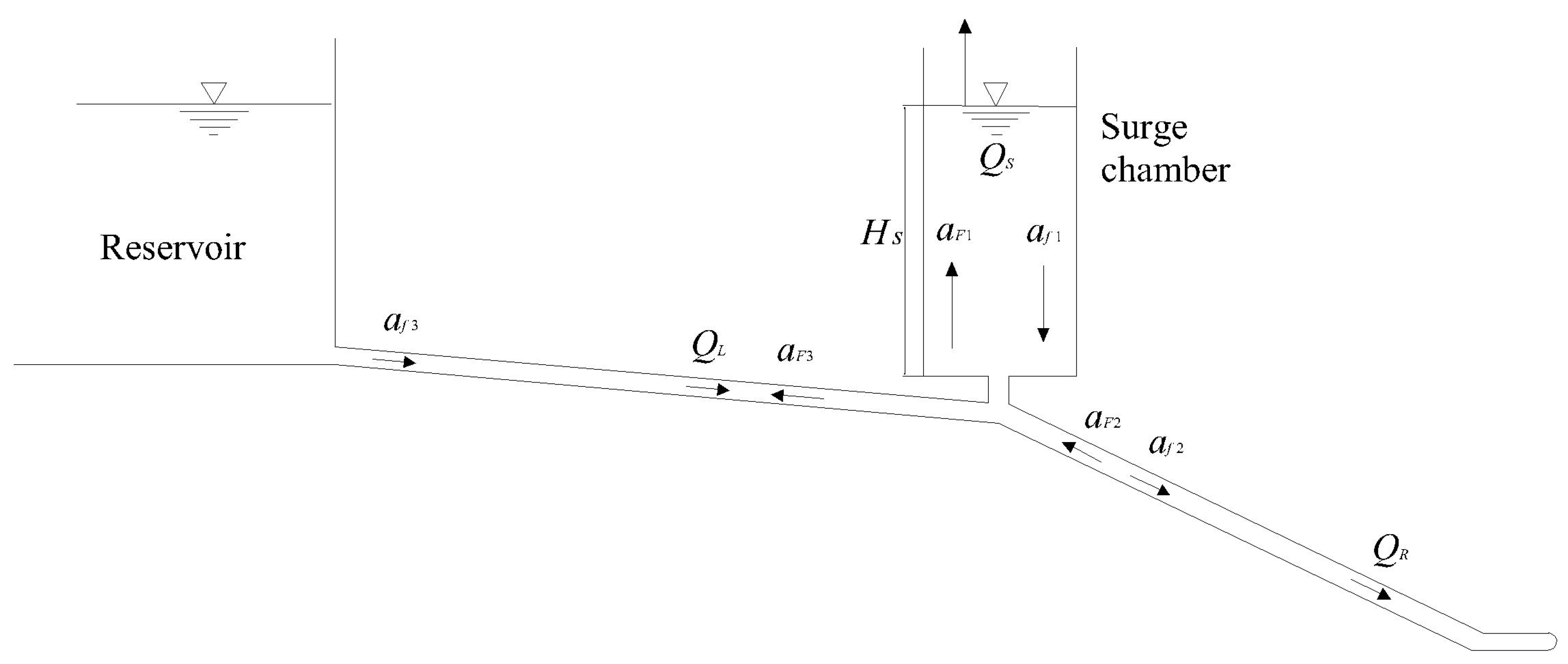
In a surge chamber steup, the water conveyance pipeline is long, while the axial length occupied by the surge chamber is relatively shorter. Therefore, the surge chamber can be equivalent to a particle with the same function and quality [27]. A schematic of the surge chamber is presented in Figure 1.
A surge chamber follows the basic equation [19],
where QL denotes the flow at the upstream end adjacent to the surge chamber, QR denotes the flow across the section shortly downstream the chamber and Qs denotes the exchanged flow between the surge chamber and the pipeline. As a result of the FSI response, the velocity of the fluid in the surge chamber is actually the one relative to the lateral vibration velocity of the surge chamber. The motion and continuity equation of the surge chamber can be defined as in Equation (10)
where As and Hs, separately, denote the section area and dynamic water level of the surge chamber. In consideration of the FSI, the velocities corresponding to QL and QR separately are taken as the relative ones to the pipe vibration speed. The following equation is then obtained
Considering the lateral coupling vibration of the pipeline, the water level in the surge chamber is taken as the relative value of the piezometric head in the chamber compared to the lateral displacement of the pipeline. As shown in Appendix A, the P at n + 1 time–step is obtained as follows.
The motion and equilibrium equations for lumped mass and inner fluid in the axial z direction satisfy.
Meanwhile, the motion equation in plane Z–Y and the equilibrium equations satisfy
where subscript L denotes the pipe nearest to the end of the pipeline upstream the chamber, subscript R denotes the computation node nearest to the head end of the pipeline downstream the chamber, mV represents the mass of the surge chamber and J represents the rotating inertia of the lumped mass block around the x–axis.
2.3. Elbow Tube
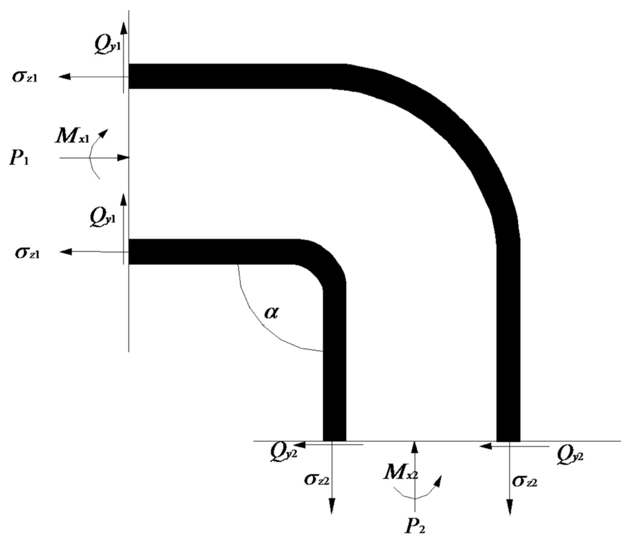
The fluid state forcibly changes at the elbow tube, and the local coupling taking place here significantly influences the FSI response of the water conveyance system. The junction coupling at elbows is illustrated in Figure 2.
At the elbow of the pipeline, the coupling is treated as a boundary condition [28] by ignoring the local head loss. The pressure balance relationship at both ends of the elbow junction can be expressed as [29]
P1 = P2
By ignoring the flow separation and considering the continuity of the water column, the equilibrium equation of flow velocity and the velocity on the wall can be computed as
V1 − uz1 = V2 − uz2
Meanwhile, the motion equations are
Af P1 − As σz1 = (Af P2 − As σz2) cosα + Qy2 sinα
Qy1 = (Af P2 − As σz2) sinα + Qy2 cosα
Mx1 = Mx2
2.4. Outlet and Inlet Boundary
Given that the cross–sectional area of the reservoir is much larger than that of the pipeline, the water level in the tank can be treated as a constant [30]
where P0 denotes the pressure provided by the water level in the reservoir. The pipeline is rigidly connected to the water tank. When the inlet or outlet is connected rigidly, continuity equations of axial, lateral, and bending directions are as follows [31]
P = P0
uz = 0
uy = 0
θx = 0
If the outlet is free, then the pipeline vibrates. Considering the FSI response, its unit discharge is taken as the relative value between the actual flow velocity in the pipeline and its axial velocity. The flow equation then can be modelled as
With a free outlet, considering the mass of valve, the equilibrium equations of the axial, lateral, and angular forces at the outlet of the pipeline are, respectively, obtained as
where Δt denotes the time step length and Δuz, Δuy and Δθx represent the variations in the axial and lateral velocities at the outlet of pipeline and the variation in the turning angle during a time step, respectively.
3. Solution Technique
3.1. Finite Volume Method
When the equations are expressed in a discrete form by the finite volume method (FVM), the physical explanation of the each term can be obtained and the conservation property of the discrete equation is satisfied. This numerical method has relatively high accuracy because it performs integration in each control volume. Subsequently, the FSI with water hammer in the pipeline is calculated. It achieves dispersion of the equations with the control volume integral and integrates the continuous equation from t to t + Δt [32,33]. From Equations (1)–(8), the continuity and momentum equations of the water region and structure region can be written in the matrix form.
The discretization of partial differential terms is realized by using the Crank–Nicolson implicit format with the Central difference of the time [34].
The differential equation for staggered nodes can be obtained by following the same principle
where A, B and S are the matrices decided by Equations (1)–(8), and they are the matrices composed by constant. Δt is used to calculate the time step, Δz refers to the spacing between the calculation nodes of adjacent pipelines, n refers to the nth time step and i refers to the number of pipes.
According to Equation (33), the iterative matrix between adjacent time steps for the water conveyance system is built as follows:
Vector Ci refers to the state vector of calculation node in the ith pipe at the nth time step. When calculating the state vector at the (n + 1)th time step, Ci is a known parameter. Vector Qi denotes the calculation node state vector at the (n + 1)th time step in the ith pipe as obtained from the iteration of Equation (34) in the nth time step state, Qi is an unknown vector. In these equations, i = 1 to N, where 1 and N refer to the calculation nodes at the inlet and outlet of the pipeline, respectively. When the pipeline or fluid between adjacent pipe structure is discontinuous, then this pipeline or fluid will be processed as an interior boundary condition. Ai and Ci are included in the boundary condition’s equation.
3.2. Boundary Condition
If supports, elbows or additional hydraulic structures are present between the ith and (i + 1)th pipe, then the pipeline or fluid is discontinuous. In this case, the discontinuity can be processed as staggered boundary conditions. In other words, the outlet of the ith pipe is connected to the inlet of the (i + 1)th pipe, and the following equilibrium equation can be used.
Disassemble Ai, Qi and Ci, then
Expansion is obtained at the ith pipe, and the structure causes the system’s state to change suddenly. Then, the motion equations are obtained as Equation (37) and Equation (38), separately.
Similarly, by decomposition of matrix Ci according to Equation (34), the following equation is obtained.
where T1 and T2 denote the coefficient matrices of the boundary condition’s equations at the inlet and outlet, respectively. It is notable that Equation (34) is an iterative formula of a water conveyance system without elbows, auxiliary buildings, or supports. In the method used in this study, elbows, auxiliary buildings, or supports are taken as boundary conditions, and the relevant iterative formula is obtained by substituting Equation (39) into Equation (34). The iterative formula is complex, especially the first term of Equation (34). Thus, a computing code was programmed by the first author to perform the complex matrix calculations.
4. Experimental Verification
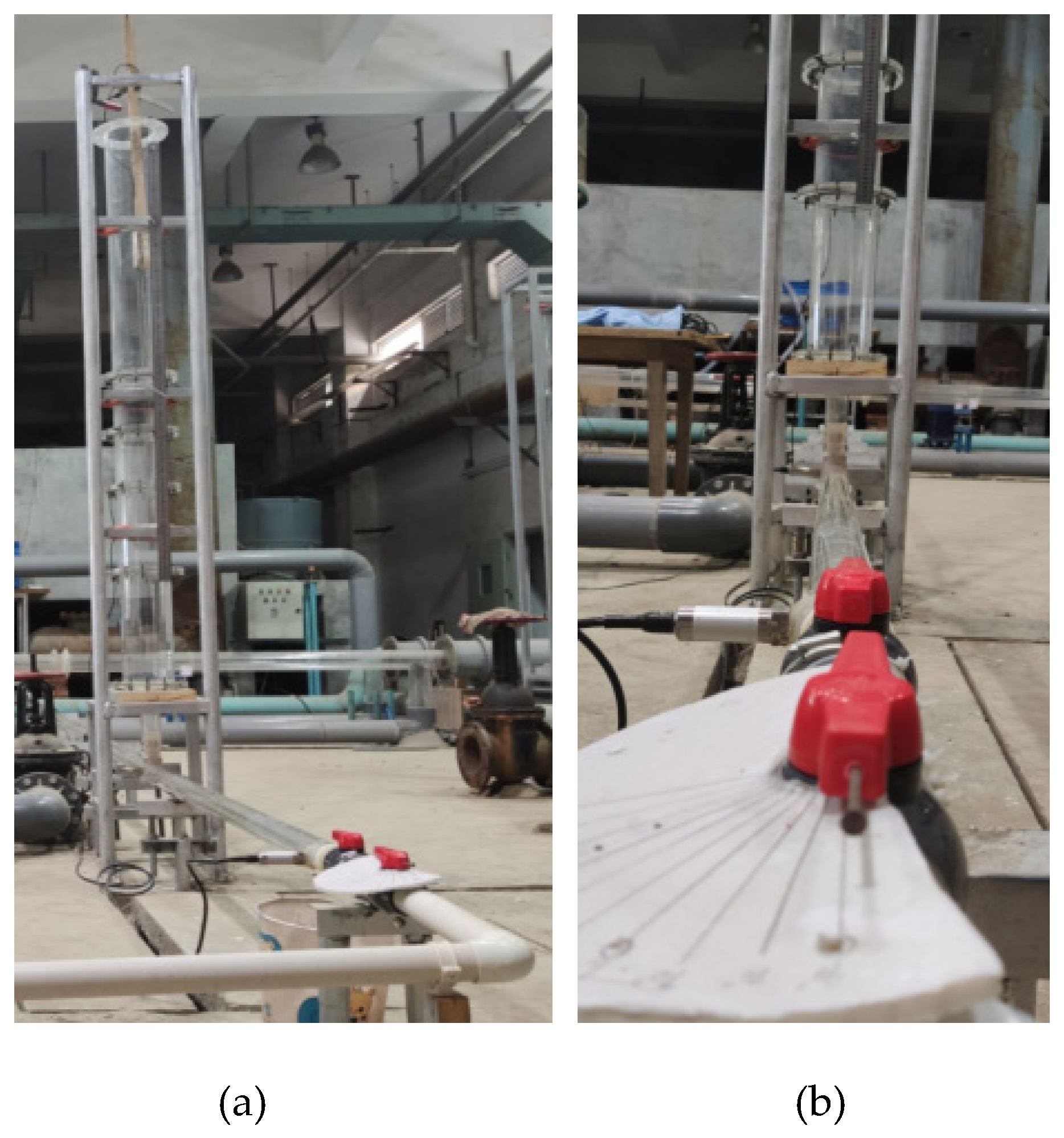
To verify the suitability and rationality of the numerical model for the FSI of a water conveyance system with a surge chamber, the experimental data were obtained and compared. The experimental device was a reservoir–pipe(PVC)–valve system with a surge chamber, as shown in Figure 3 and Figure 4. Pipeline parameters are shown in Table 1.
The model has few supports and shows a strong coupling response [31]. The experimental phenomena were obvious. An HQ1000 pressure sensor was used to record the history of coupling pressure pulsation in the Z–type pipeline. Pressure sensors with 1000 Hz sampling frequency were installed near the valve end and at the bottom of the surge chamber. According to [19], the water hammer wave velocity was computed as cf = 1128 m/s, the frequency is computed as f =cf /4 L = 25.41 Hz, the stress wave velocity was cs = 2557 m/s and the time cycle was f =cs/4 L = 53.19 Hz. A data acquisition frequency of 200 Hz could reflect the stress and pressure waves. The pipeline vibration frequency was far less than the calibration frequency of the pressure sensor and did not cause resonance. Therefore, the pressure sensor in this experiment was considered to be suitable.
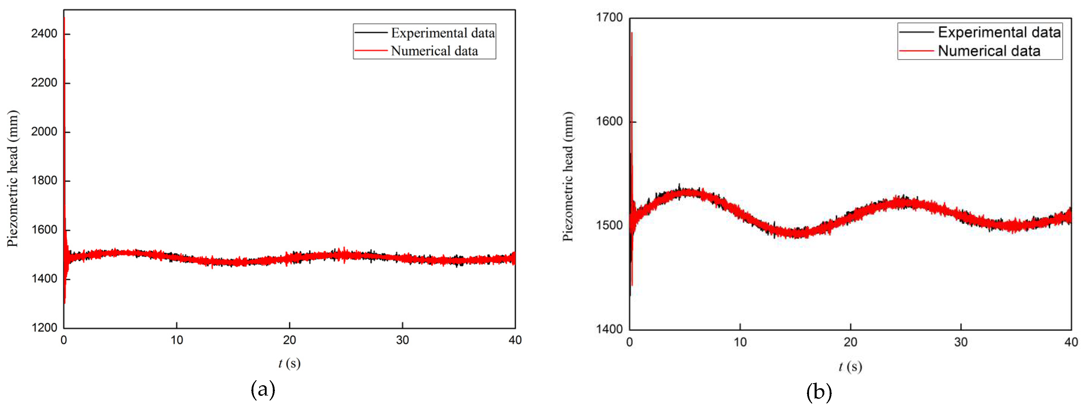
A water conveyance pipeline with a surge chamber has a complex coupled response. When the valve is closed, a stress wave and pressure wave are produced, and they interact mutually. Afterwards, a surge takes place in the surge chamber induced by pressure wave. From Equations (10) to (15), considering FSI, the downstream of surge chamber has considerable discharge and there is an in-negligible pipe–wall vibration near surge chamber. Meanwhile, a stress wave and a pressure wave are produced. At the closed valve, the discharge changes suddenly, so the stress and pressure waves are also induced.
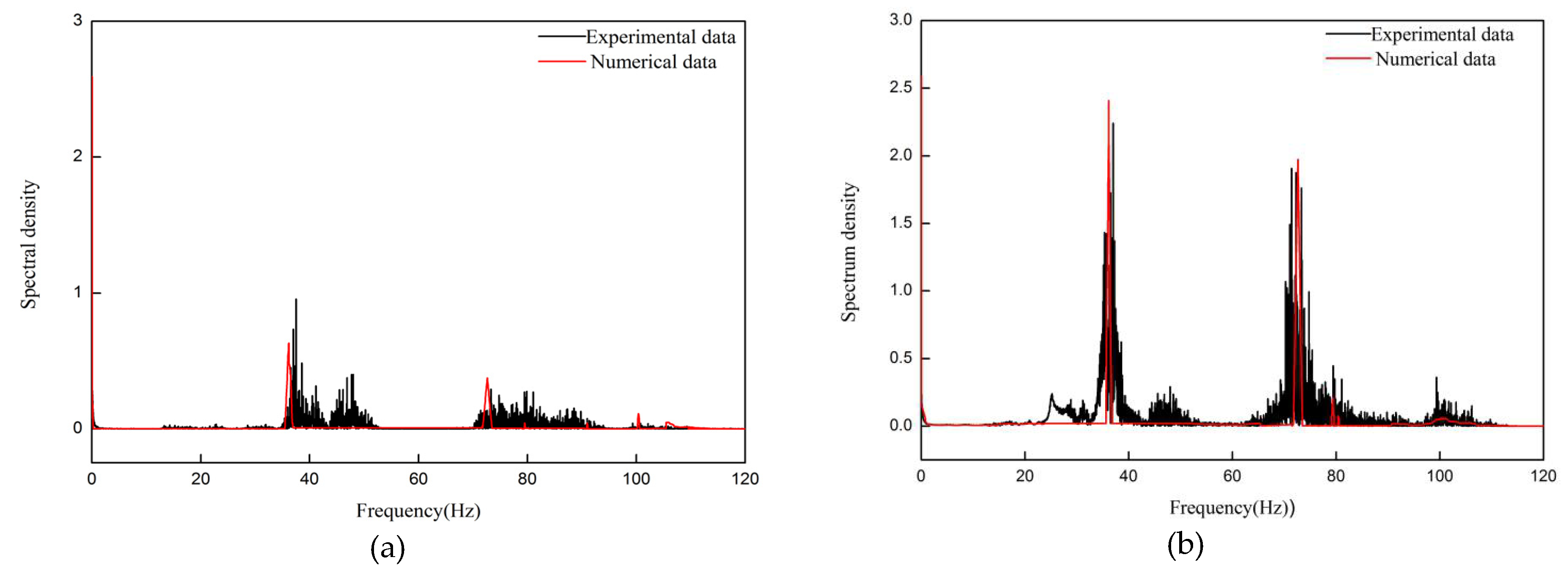
Thus, the surge acts as an exciting source to cause pulsation waves at the closed valve. A long–term surge leads to the durable FSI responses. But the energy of the pressure wave is greatly reduced due to the reflecting function of surge chamber. In this study, it was assumed that the pressure wave propagates only between surge chamber and valve. The frequency of the pressure wave fp = cf/4d = 72.63 Hz (d = 2 m) and the frequency of stress wave fs = cs/4 L = 38.37 Hz. The time domain of the FSI response in the whole process is shown in Figure 5a,b. The results of fast Fourier transformation are displayed in Figure 6a,b. The pressure fluctuation was composed of the stress wave, pressure wave, and gravity wave (surge). A comparison of Figure 6a,b reveals that, for the pipe closer to the surge chamber, the gravity wave contributed more to the pressure pulsation amplitude because energy losses occur during the propagation of the stress and water hammer waves.
Only the stiffness and axial friction coefficient of the pipeline support were estimated in this paper. The downstream valve was still part of the water conveyance system (Figure 4), and the stress wave propagated downward through the valve. However, this segment of pipeline is ignored in the current computation model. This model was simplified and has less influence. The model was solved by FVM, so numerical results are only approximate and differ from the actual values.
The water reservoir in a surge chamber setip has a small sectional area. Admittedly, after performing a series of measurements, the water level in the tank had a weak fluctuation. The small inertia of the tank and the pipeline vibration are likely to cause the water tank to vibrate. Given the uncertainty of errors from the operators, the experimental environment and the pressure sensor, the numerical results differed from the experimental data. However, the comparison of the experimental results with the numerical results in Figure 5 and Figure 6 revealed that these two sets of data were in good agreement with each other, thereby validating the suitability and rationality of the proposed computational model.
5. Numerical Results and Discussion
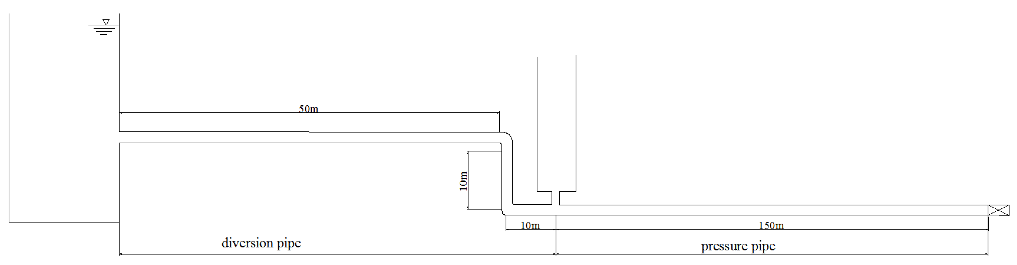
In this section, water hammer with FSI in a water conveyance system with a surge chamber is described. The pipeline system is composed by two horizontal pipes with lengths of 50 m and 160 m, and they are connected by a 10 m vertical pipe. In this study, the deflection of the pipeline was ignored. A reservoir was at the inlet of the system, a valve was at the outlet of the system. The inner diameter and wall thickness of the pipeline ware 2 m and 0.05 m, respectively. The surge chamber was installed near the elbow pipe, and this system had an initial flow rate and initial pressure of 1 m3/s and 0.4 MPa, separately. The cross–section areas of the surge chamber and impedance hole were 11 m2 and 3 m2. The schematic of the water conveyance system is shown in Figure 7. The governing equation was built by using a universal FVM. Given the very small frequencies of the stress and water hammer waves, a relatively large calculation time step could be selected. However, to ensure the reliability of the numerical results, the calculation time step could not be too large.
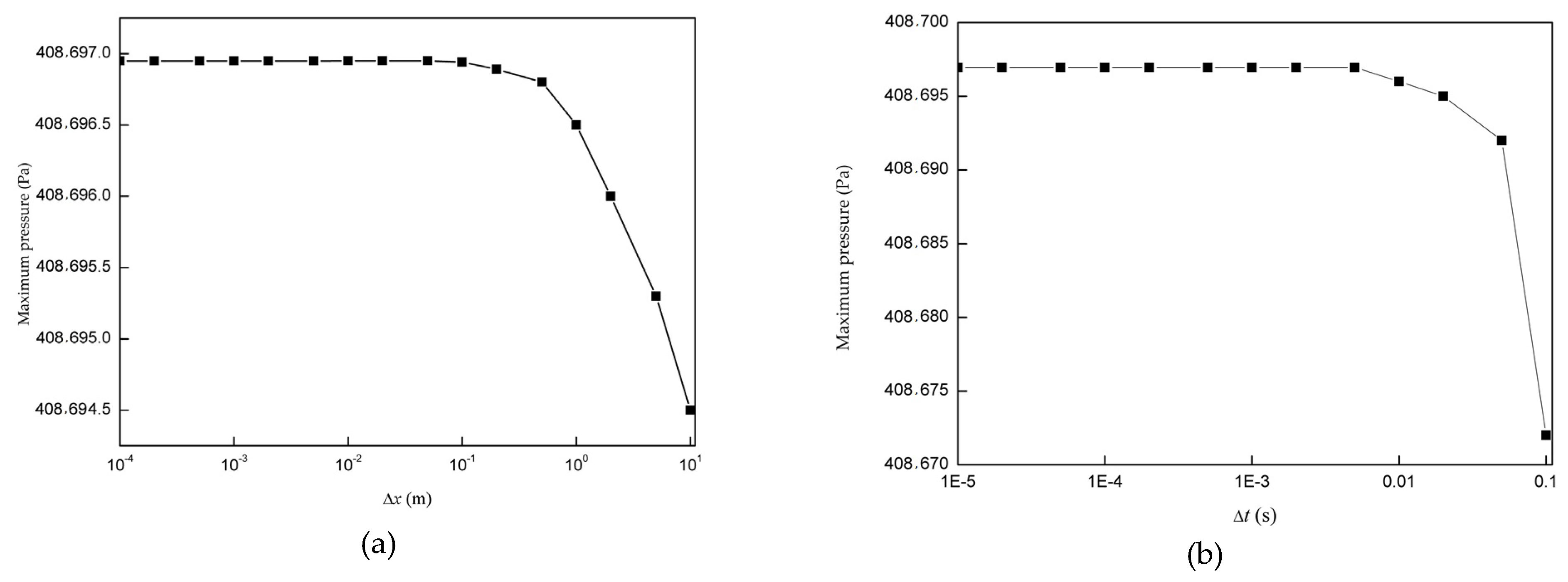
The numerical results of maximum pressure vary with mesh size is given in Figure 8a. When Δx > 0.1 m, the differences of numerical results with different Δx were nonignorable. And if Δx < 0.1, the differences were acceptable and ignorable, but they consumed more computing resources. With a similar law, they consume more resources with smaller Δt. When water hammer was induced by rapid closing valve, the frequencies of the FSI response of the system were less than 200 Hz. So Δt = 0.005 s as shown in Figure 8b. Following a comprehensive consideration, the pipeline spacing and calculation time step were set to 0.1 m and 0.005 s, respectively.
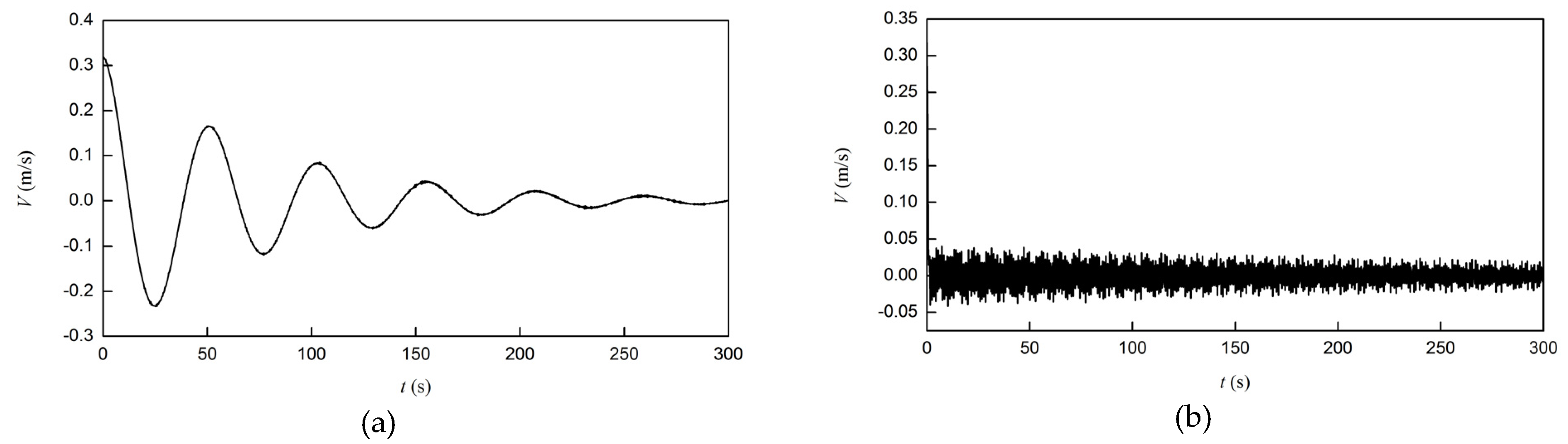
In this system, both valve closing and the subsequent water level oscillation in the surge tank were the excitation of the transition process. The surge disturbed the fluid, resulting in a non–negligible fluid velocity downstream the chamber (from Equation (12)), and junction coupling occurred at the bottom of surge chamber. This velocity caused pressure pulsation and further induced FSI. The velocity fluctuations shortly upstream and downstream the surge chamber are shown in Figure 9a,b, separately.
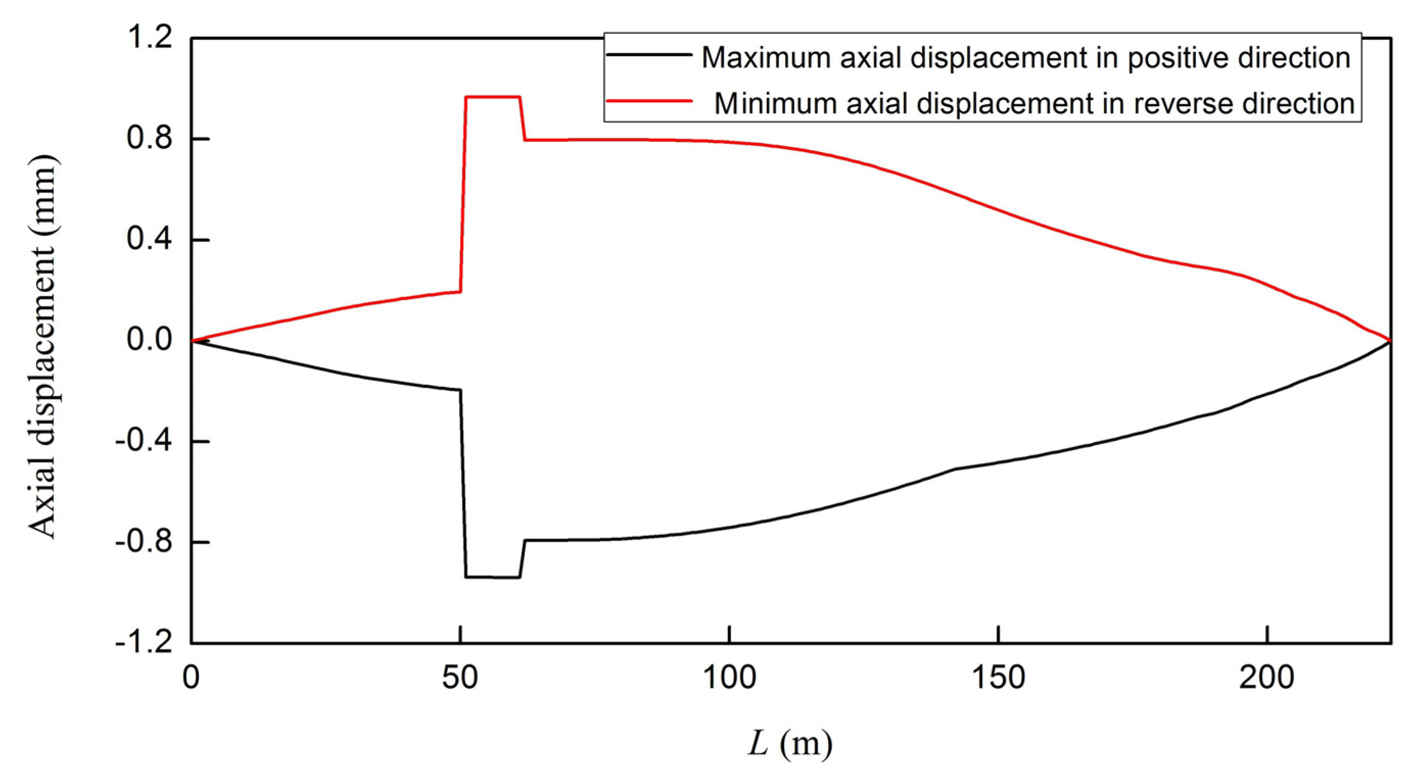
At the bottom of the surge chamber, the dynamic pressure caused the vibration of the pipe, resulting in junction coupling, and in turn a new pressure wave was produced by junction coupling in the chamber. Considering FSI, the fluid was disturbed. The pressure wave and stress wave also produced at the closed outlet, and they mutually interacted along the pipeline. The stress wave and pressure wave produced by the surge and the closed valve were superimposed with each other. With RfV and Rtuz in Equations (1) and (3), the original vibrations of pipe wall are shown in Figure 10.
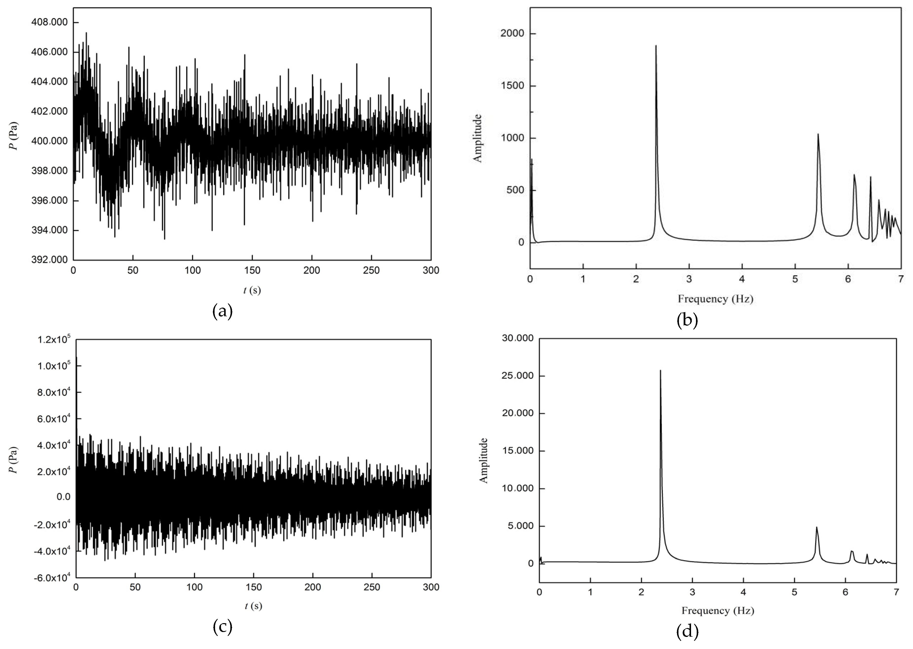
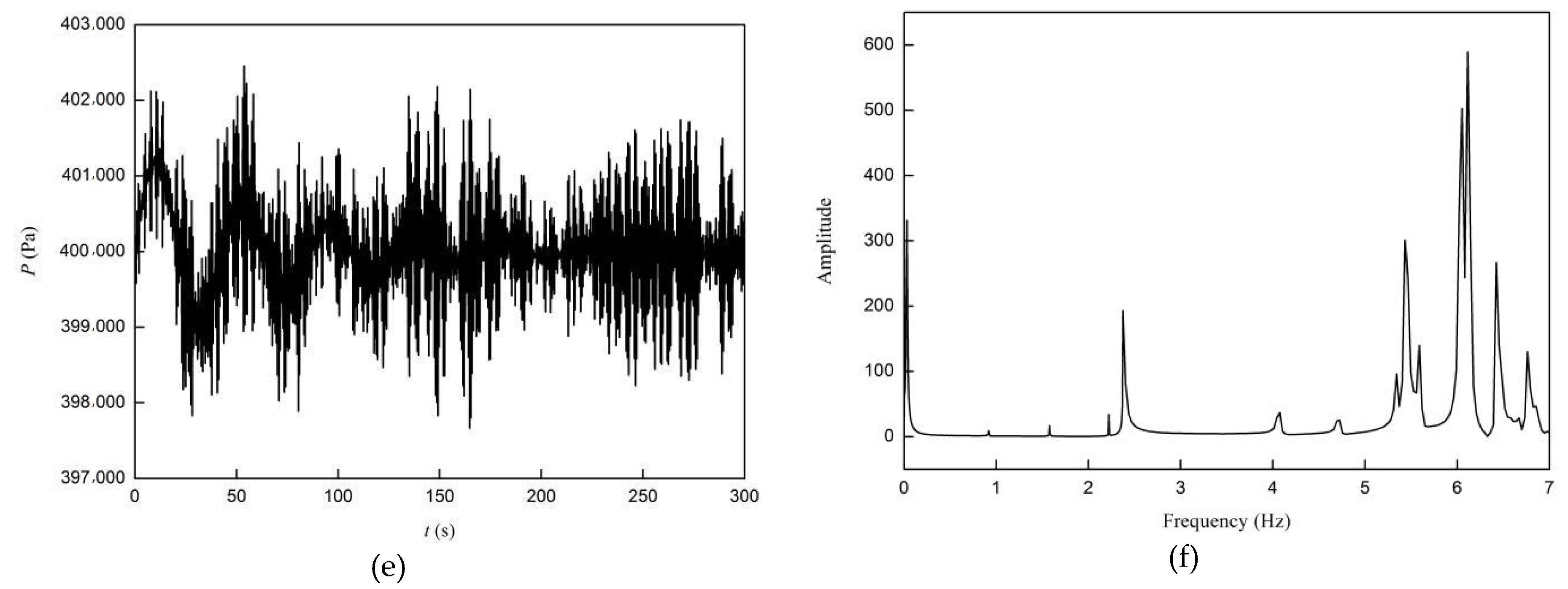
Considering FSI, the modes of elbows vibration were agreed with the modes of fluid [35]. Theoretically, the modes of the pipe have higher frequency than fluid in a water conveyance system. Thus, when elbows disturb the fluid, the pressure fluctuation with larger frequencies is produced, and it propagates throughout the pipe. The dynamic pressure at the elbow, near the surge chamber, and at the outlet are shown in Figure 11 in the time and frequency domains. Thus, the high-frequency pulsation produced by elbows plays an important role. Thus, the pressure fluctuation may be composed of a gravity wave, stress wave, pressure wave, and high frequency wave caused by elbows. Because of frictional coupling, the closer to the elbow the fluid is, the stronger the high frequency energy is, and the more important the high frequency plays.
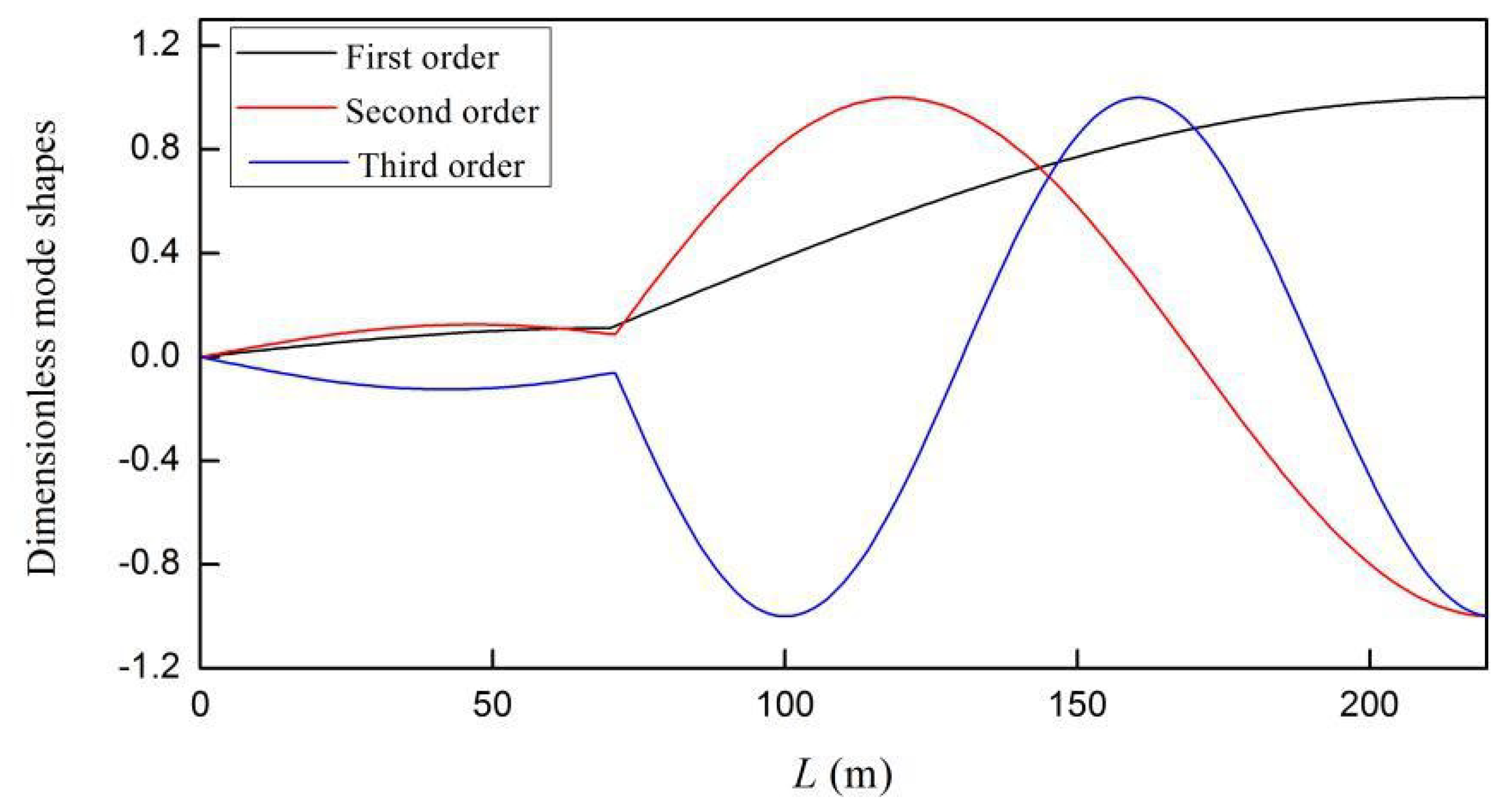
When ν = 0.3, Poisson coupling and junction coupling both exit in the system. When ν = 0, there is no Poisson coupling, and all the boundary conditions may cause junction coupling. Because Poisson coupling results in faster pipe expansion or contraction, each mode of fluid has a higher frequency when ν = 0.3. The first three mode shapes and the first seven modal frequencies are shown in Figure 12 and Table 2, separately.
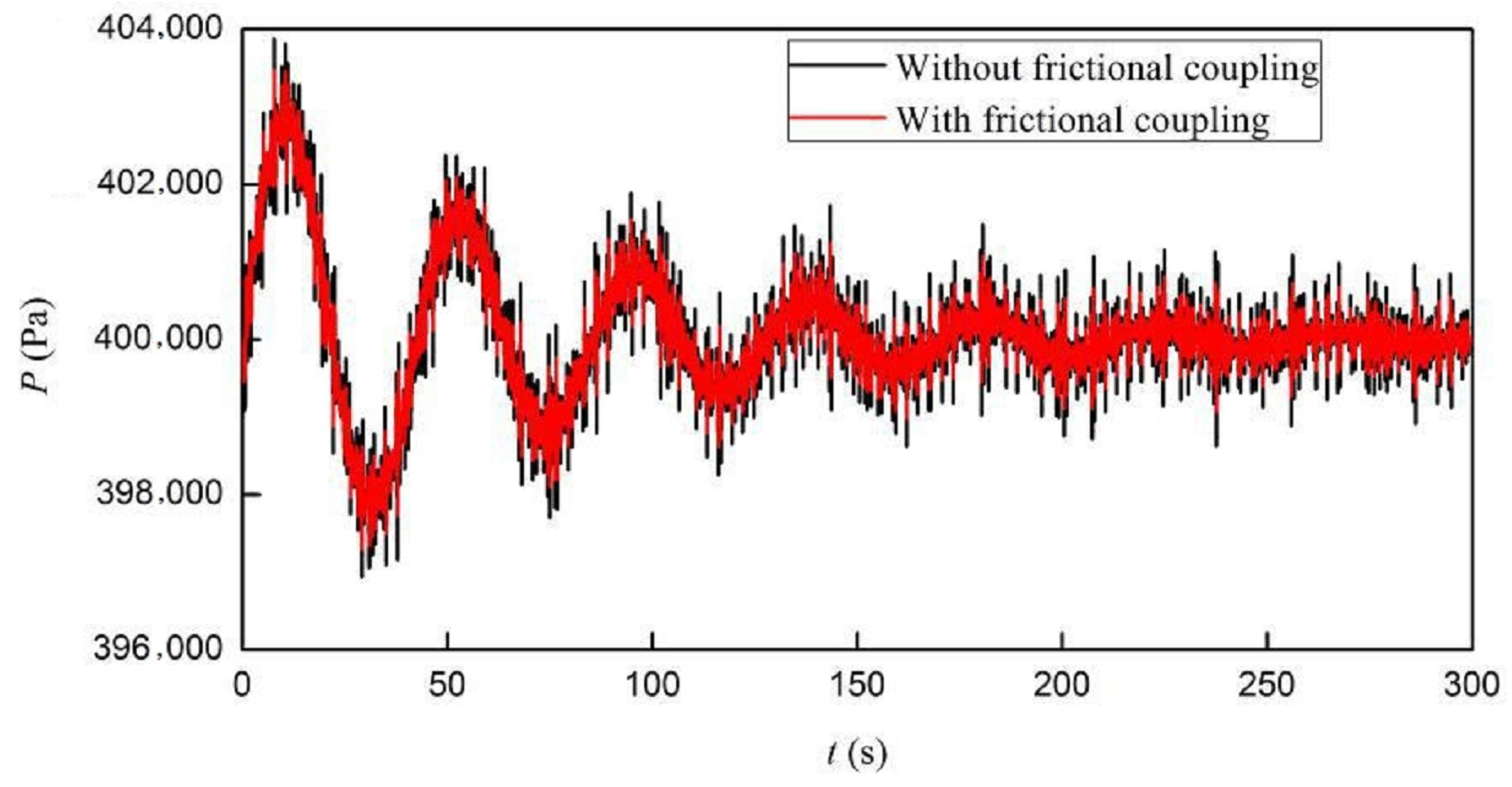
Considering frictional coupling, there are fluid viscous damping and structural damping in the water delivery system, which directly act on the fluid velocity and the axial vibration velocity of the pipe wall, as shown in terms of RfV and Rtuz in Equations (1) and (3). Without fractional coupling, Rtuz equals zero. The numerical results of pressure with and without fractional coupling are shown as the red solid line and the black solid line respectively in Figure 13. With fractional coupling, the disturbance mainly comes from lower axial displacement. So the fluid fluctuations with frequencies of stress wave and pressure wave have a smaller amplitude.
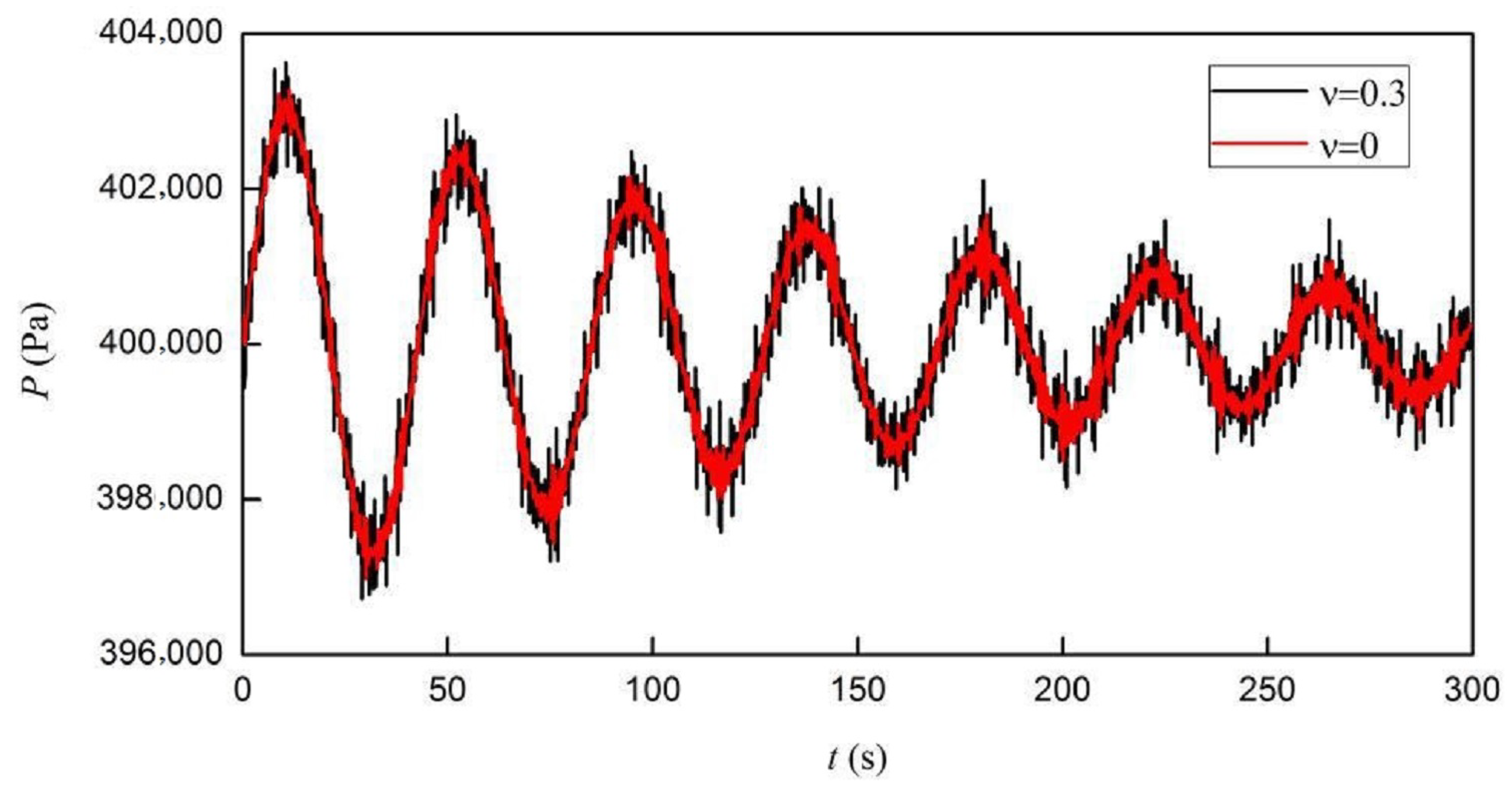
As for Poisson coupling, its influence on the water conveyance system is represented by 2ν/E in Equation (2) and νR/Ee in Equation (4), respectively. Considering Poisson coupling, the amplitude of local transiliences of the dynamic pressure curve are increased, as shown in Figure 14.
6. Conclusions
The fact that this study takes the water-hammer-structure interaction into account distinguishes it from the existing literature about water conveyance systems with a surge chamber. In this study, the water pipeline system was in a plane, and it is appropriate that the couplings in the plane were decoupled with the couplings out of the plane. Considering the axial and lateral motion of the pipe in the plane, the system state was described by eight variables. So, this paper presented the FSI eight equation model. Bends and the surge chamber were taken as boundary conditions, and they were numerically solved by FVM. The numerical results were in good agreement with the experimental ones. It was proved that FVM is suitable for generating numerical solutions and that the model is reasonable.
The excitations considered in this paper are water level oscillation in the surge chamber and valve closing. When the valve is closed, surge emerges in the system and lasts for a long time. Considering FSI, junction coupling produced by surge at the bottom of surge chamber will cause a notable change of discharge downstream the surge chamber and a non-negligible axial stress wave. This wave in turn causes a new pressure wave. At the closed valve, the discharge changes suddenly, and a stress wave and a pressure wave are also induced. Pressure fluctuation is the superposition of surge, stress wave, and pressure wave.
Considering FSI, the fluid pulsation in the system is composed of stress waves, pressure waves, gravity waves, and some high-frequency waves produced by elbows. Because frequencies of others are much higher than the gravity wave, there are multiple local mutations on the pressure dynamic curve. FSI can be divided into three types: friction coupling, Poisson coupling, and junction coupling. Junction coupling occurs at the bottom of surge chamber, elbow, and valve, causing pressure waves and stress waves, and further inducing Poisson coupling. In the long–term transition process, friction coupling is an important mechanism of FSI, affecting the amplitude of transiliences on the pressure curve.
From these results, firstly, local transiliences emerging in the numerical pressure signal may be induced by water–hammer–structure interaction, not by false hydraulic vibration; secondly, considering FSI, the numerical results are more authentic and the peak is larger. Thus, they play important roles in the orifice optimization of the surge chamber.
In this paper, it was considered that the structure inertia of surge tank is large enough without influence of the changing water level. In the future, surge chambers made of light materials could be studied, and the inertia varying with the water level in the chamber could also be considered. Considering the dynamic inertia of the surge chamber, some interesting results will be obtained.
Author Contributions
Conceptualization, Q.G.; methodology, Q.G.; validation, D.L.; investigation, X.G.; resources, J.Z. (Jianxu Zhou); data curation, Y.L.; formal analysis, Q.G.; writing—original draft preparation, Q.G. writing—review and editing, Q.G. and J.Z. (Jian Zhang); All authors have read and agreed to the published version of the manuscript.
Funding
This work was supported by the National Natural Science Foundation of China (Grant Nos. 51879087, 51839008 and 51709087).
Acknowledgments
The authors gratefully acknowledge all the help from all the Research Institute of Hydraulic and Hydropower Engineering.
Conflicts of Interest
The authors declare no conflict of interest.
Appendix A
From Equation (11)
Equation (A1) multiply Δt/2As, reduced by Equation (A2), Equation (A3) is obtained
Substitution Equation (9) into Equation (A3)
For n + 1 time step, the state of n time step is known. For convenience, suppose
References
- Leishear, R.A. Fluid Mechanics, Water Hammer, Dynamic Stresses, and Piping Design; ASME: New York, NY, USA, 2012. [Google Scholar] [CrossRef] [Green Version]
- Olalla, G.; SasIrene, D.; Begoña, G. Liquid-liquid extraction of phenolic compounds from water using ionic liquids: Literature review and new experimental data using C2mim FSI. J. Environ. Manag. 2018, 78, 475–482. [Google Scholar] [CrossRef]
- Osama, M.; Theofilis, V.; Ahmed, E. Fluid Structure Interaction (FSI) Simulation Of the human eye under the air puff tonometry using CFD. In Proceedings of the Tenth International Conference on Computational Fluid Dynamics (ICCFD10), Barcelona, Spain, 9–13 July 2018. [Google Scholar]
- Bazilevs, Y.; Yan, J.; Deng, X. Simulating Free-Surface FSI and Fatigue Damage in Wind-Turbine Structural Systems. In Frontiers in Computational Fluid-Structure Interaction and Flow Simulation: Research from Lead Investigators under Forty; Springer: Berlin, Germany, 2018. [Google Scholar] [CrossRef]
- Tijsseling, A.S.; Vardy, A.E. Time scales and FSI in unsteady liquid-filled pipe flow. In The 9th International on Pressure Surges; Chester, UK, 2004. [Google Scholar] [CrossRef]
- Wiggert, D.C.; Hatfield, F.J.; Stuckenbruck, S. Analysis of Liquid and Structural Transients in Piping by the Method of Characteristics. J. Fluids Eng. 1987, 109, 161–165. [Google Scholar] [CrossRef]
- Lavooij, C.S.W.; Tijsseling, A.S. Fluid–structure interaction in liquid-filled piping systems. J. Fluids Struct. 1991, 5, 573–595. [Google Scholar] [CrossRef]
- Ahmadi, A.; Keramat, A. Investigation of fluid–structure interaction with various types of junction coupling. J. Fluids Struct. 2010, 26, 1123–1141. [Google Scholar] [CrossRef]
- Liu, Y.; He, X.; Zhi, Y. Dynamical strength and design optimization of pipe-joint system under pressure impact load. Proceedings of the Institution of Mechanical Engineers, Part G. J. Aerosp. Eng. 2011, 226, 1029–1040. [Google Scholar] [CrossRef]
- Huang, S.; Zhou, B.; Bu, S.; Li, C.; Zhang, C.; Wang, H.; Wang, T. Robust fixed-time sliding mode control for fractional-order nonlinear hydro-turbine governing system. Renew. Energy 2019, 139, 447–458. [Google Scholar] [CrossRef]
- Zhai, H.; Wu, Z.; Liu, Y.; Yue, Z. In-plane dynamic response analysis of curved pipe conveying fluid subjected to random excitation. Nucl. Eng. Des. 2013, 256, 214–226. [Google Scholar] [CrossRef]
- Tijsseling, A.S.; Vardy, A.E.; Fan, D. Fluid-Structure Interaction and Cavitation in a Single-elbow Pipe System. J. Fluid Struct. 1996, 10, 395–420. [Google Scholar] [CrossRef]
- Mu, L.Z.; Li, X.Y.; Chi, Q.Z.; Yang, S.Q.; Zhang, P.D.; Ji, C.J.; He, Y.; Gao, G. Experimental and numerical study of the effect of pulsatile flow on wall displacement oscillation in a flexible lateral aneurysm model. Acta Mech. Sin. 2019, 39, 1120–1129. [Google Scholar] [CrossRef]
- Forbes, T.B.; Stephen, C.T. Dynamic Behavior of Complex Fluid-Filled Tubing Systems-Part ii: System Analysis. J. Dyn. Syst. Meas. 2001, 123, 78–84. [Google Scholar] [CrossRef]
- Altstadt, E.; Carl, H.; Prasser, H.M.; Weis, R. Fluid-structure interaction during artificially induced water hammers in a tube with a bend—Experiments and analyses. Multiph. Sci. Technol. 2008, 20, 213–238. [Google Scholar] [CrossRef]
- Wang, Y.G. Efficient prediction of wave energy converters power output considering bottom effects. Ocean Eng. 2019, 181, 89–97. [Google Scholar] [CrossRef]
- Zhang, Y.L.; Miao, M.F.; Ma, J.M. Analytical study on water hammer pressure in pressurized conduits with a throttled surge chamber for slow closure. Water Sci. Technol. 2010, 3, 174–189. [Google Scholar] [CrossRef]
- Chen, S.; Zhang, J.; Yu, X.D. Characterization of surge superposition following 2-stage load rejection in hydroelectric power plant. Can. J. Civ. Eng. 2016, 43, 844–850. [Google Scholar] [CrossRef]
- Guo, W.C.; Yang, J.D. Combined effect of upstream surge chamber and sloping ceiling tailrace tunnel on dynamic performance of turbine regulating system of hydroelectric power plant. Chaos Solitons Fractals 2017, 99, 243–255. [Google Scholar] [CrossRef]
- Zhang, Y.L.; Niao, M.F. Explicit formulas for calculating surges in throttled surge chamber. J. Hydraul. Eng. 2012, 4, 467–472. (In Chinese) [Google Scholar]
- Wiggert, D.C.; Otwell, R.S.; Hatfield, F.J. The effect of elbow restraint on pressure transients. J. Fluid Eng. 1985, 107, 402–406. [Google Scholar] [CrossRef]
- Okosun, F.; Cahill1, P.; Hazra, B.; Pakrash, V. Vibration-based leak detection and monitoring of water pipes using output-only piezoelectric sensors. Eur. Phys. J. Spec. Top. 2019, 228, 1659–1675. [Google Scholar] [CrossRef]
- Tijsseling, A.S.; Wiggert, D.C. Fluid transients and fluid-structure interaction in flexible liquid-filled pipeing. Appl. Mech. Rev. 2001, 54, 455–481. [Google Scholar] [CrossRef]
- Wang, Y.H.; Zhang, J.H.; Ma, Z.X. Experimental determination of single-phase pressure drop and heat transfer in a horizontal internal helically-finned tube. Int. J. Heat Mass Transf. 2017, 104, 240–246. [Google Scholar] [CrossRef]
- Taitel, Y.; Dukler, A.E. A model for predicting flow regime transition in horizontal and near horizontal gas-liquid flow. AIChE J. 1976, 22, 47–55. [Google Scholar] [CrossRef]
- Meindlhumer, M.; Pechstein, A. 3D mixed finite elements for curved, flat piezoelectric structures. Int. J. Smart Nano Mater. 2019, 10, 249–267. [Google Scholar] [CrossRef] [Green Version]
- Wei, X.; Sun, B. Study on fluid–structure interaction in liquid oxygen feeding pipe systems using finite volume method. Acta Mech Sin. 2011, 27, 706–712. [Google Scholar] [CrossRef]
- Ferras, D.; Manso, P.A.; Covas, D.I.C. Fluid–structure interaction in pipe coils during hydraulic transients. J. Hydraul. Res. 2017, 55, 491–505. [Google Scholar] [CrossRef]
- David, F.; Pedro, A.M.; Anton, J.S. Fluid-structure interaction in straight pipelines with different anchoring conditions. J. Sound Vib. 2017, 394, 348–365. [Google Scholar] [CrossRef]
- Banks, J.W.; Henshaw, W.D.; Schwen, D.W. A stable partitioned FSI algorithm for rigid bodies and incompressible flow in three dimensions. J. Comput. Phys. 2018, 73, 455–492. [Google Scholar] [CrossRef] [Green Version]
- Li, S.J.; Karney, B.W.; Liu, G.M. FSI research in pipeline systems-A review of the literature. J. Fluids Struct. 2015, 57, 277–297. [Google Scholar] [CrossRef]
- Ramírez, L.; Nogueira, X.; Ouro, P. A Higher-Order Chimera Method for Finite Volume Schemes. Arch. Comput. Methods Eng. 2018, 25, 691–706. [Google Scholar] [CrossRef] [Green Version]
- Hwang, Y.H.; Chung, N.M. A fast Godunov method for the water-hammer problem. Int. J. Numer. Methods Fluids 2002, 40, 799–819. [Google Scholar] [CrossRef]
- Sreejith, B.; Jayaraj, K.; Ganesan, N. Finite element analysis of fluid-structure interaction in pipeline systems. Nucl. Eng. Des. 2004, 227, 313–322. [Google Scholar] [CrossRef]
- Zhang, L.; Tijsseling, A.S.; Vardy, E.A. FSI analysis of liquid-filled pipes. J. Sound Vib. 1999, 224, 69–99. [Google Scholar] [CrossRef] [Green Version]
Figure 1.
Schematic of a surge chamber (aF is transmitted wave and af is reflected wave).

Figure 2.
Definition sketch of the junction coupling in elbow.

Figure 3.
The experimental equipment. (a) is the graph of piping system and (b) is the graph of pressure sensor.
Figure 3.
The experimental equipment. (a) is the graph of piping system and (b) is the graph of pressure sensor.

Figure 4.
Schematic of water conveyance system with surge chamber.

Figure 5.
Pressure fluctuation history with fluid–structure interaction (FSI) taking into account (a) closer outlet; (b) near surge chamber. The red solid line refers to numerical result, the black solid line refers to experimental result.
Figure 5.
Pressure fluctuation history with fluid–structure interaction (FSI) taking into account (a) closer outlet; (b) near surge chamber. The red solid line refers to numerical result, the black solid line refers to experimental result.

Figure 6.
Pressure in frequency domain with FSI taking into account (a) closer outlet; (b) near surge chamber. The red solid line refers to numerical result, the black solid line refers to experimental result.
Figure 6.
Pressure in frequency domain with FSI taking into account (a) closer outlet; (b) near surge chamber. The red solid line refers to numerical result, the black solid line refers to experimental result.

Figure 7.
Schematic of water conveyance system with surge chamber.

Figure 8.
Verification of mesh independent.(a): verification of Δx, (b): verification of Δt

Figure 9.
Time history of flow velocity near surge chamber, (a) upstream, (b) downstream.

Figure 10.
Amplitude of original modes of axial displacement of pipe produced by surge and closed valve.
Figure 10.
Amplitude of original modes of axial displacement of pipe produced by surge and closed valve.

Figure 11.
Time history and frequency responses of dynamic pressure. (a,c,e) are time histories of dynamic pressure near surge chamber, at the outlet and at the elbow. (b,d,f) are frequency responses of dynamic pressure near surge chamber, at the outlet and at the elbow.
Figure 11.
Time history and frequency responses of dynamic pressure. (a,c,e) are time histories of dynamic pressure near surge chamber, at the outlet and at the elbow. (b,d,f) are frequency responses of dynamic pressure near surge chamber, at the outlet and at the elbow.


Figure 12.
Mode shapes of first-three orders.

Figure 13.
Time history of pressure at the bottom of surge chamber with and without frictional coupling.
Figure 13.
Time history of pressure at the bottom of surge chamber with and without frictional coupling.

Figure 14.
Time history of pressure at the bottom of surge chamber with and without Poisson coupling.
Figure 14.
Time history of pressure at the bottom of surge chamber with and without Poisson coupling.


Table 1.
Parameters of the experimental pipeline.
| ν | E | L | e | D | ρt |
|---|---|---|---|---|---|
| 0.3 | 3.88 Gpa | 11.1 m | 0.005 m | 0.05 m | 1378.57 kg/m3 |
Table 2.
Modes of first–seven orders.
| Mode | ν = 0.3 | ν = 0 |
|---|---|---|
| 1 | 2.1 Hz | 2.1 Hz |
| 2 | 5.8 Hz | 5.6 Hz |
| 3 | 9.3 Hz | 9.0 Hz |
| 4 | 13.1 Hz | 12.7 Hz |
| 5 | 17.0 Hz | 16.1 Hz |
| 6 | 20.5 Hz | 19.7 Hz |
| 7 | 21.2 Hz | 23.1 Hz |
© 2020 by the authors. Licensee MDPI, Basel, Switzerland. This article is an open access article distributed under the terms and conditions of the Creative Commons Attribution (CC BY) license (http://creativecommons.org/licenses/by/4.0/).
Share and Cite
MDPI and ACS Style
Guo, Q.; Zhou, J.; Li, Y.; Guan, X.; Liu, D.; Zhang, J. Fluid-Structure Interaction Response of a Water Conveyance System with a Surge Chamber during Water Hammer. Water 2020, 12, 1025. https://doi.org/10.3390/w12041025
AMA Style
Guo Q, Zhou J, Li Y, Guan X, Liu D, Zhang J. Fluid-Structure Interaction Response of a Water Conveyance System with a Surge Chamber during Water Hammer. Water. 2020; 12(4):1025. https://doi.org/10.3390/w12041025
Chicago/Turabian StyleGuo, Qiang, Jianxu Zhou, Yongfa Li, Xiaolin Guan, Daohua Liu, and Jian Zhang. 2020. "Fluid-Structure Interaction Response of a Water Conveyance System with a Surge Chamber during Water Hammer" Water 12, no. 4: 1025. https://doi.org/10.3390/w12041025
Note that from the first issue of 2016, this journal uses article numbers instead of page numbers. See further details here.