Numerical Simulation of Water Renewal Timescales in the Mahakam Delta, Indonesia
by

Chien Pham Van
1,*, 
Benjamin De Brye
2,
Anouk De Brauwere
3,
A.J.F. (Ton) Hoitink
4,
Sandra Soares-Frazao
5 and
Eric Deleersnijder
6
1
Department of River Engineering and Disaster Management, Thuyloi University, 175 Tay Son, Dong Da, Hanoi 100000, Vietnam
2
Free Field Technologies (FFT), 1435 Mont-Saint-Guibert, Belgium
3
Karel de Grote Hogeschool, Chemie en Biomedische Laboratoriumtechnologie, Salesianenlaan 90, 2660 Antwerp, Belgium
4
Hydrology and Quantitative Water Management Group, Department of Environmental Sciences, Wageningen University, 6708PB Wageningen, The Netherlands
5
Institute of Mechanics, Materials and Civil Engineering (IMMC), Université Catholique de Louvain, B-1348 Louvain-la-Neuve, Belgium
6
Institute of Mechanics, Materials and Civil Engineering (IMMC) & Earth and Life Institute (ELI), Université Catholique de Louvain, B-1348 Louvain-la-Neuve, Belgium
*
Author to whom correspondence should be addressed.
Water 2020, 12(4), 1017; https://doi.org/10.3390/w12041017
Submission received: 9 March 2020
/
Revised: 30 March 2020
/
Accepted: 30 March 2020
/
Published: 2 April 2020
(This article belongs to the Special Issue Tracer and Timescale Methods for Passive and Reactive Transport in Fluid Flows)
Abstract
:Water renewal timescales, namely age, residence time, and exposure time, which are defined in accordance with the Constituent-oriented Age and Residence time Theory (CART), are computed by means of the unstructured-mesh, finite element model Second-generation Louvain-la-Neuve Ice-ocean Model (SLIM) in the Mahakam Delta (Borneo Island, Indonesia). Two renewing water types, i.e., water from the upstream boundary of the delta and water from both the upstream and the downstream boundaries, are considered, and their age is calculated as the time elapsed since entering the delta. The residence time of the water originally in the domain (i.e., the time needed to hit an open boundary for the first time) and the exposure time (i.e., the total time spent in the domain of interest) are then computed. Simulations are performed for both low and high flow conditions, revealing that (i) age, residence time, and exposure time are clearly related to the river volumetric flow rate, and (ii) those timescales are of the order of one spring-neap tidal cycle. In the main deltaic channels, the variation of the diagnostic timescales caused by the tide is about 35% of their averaged value. The age of renewing water from the upstream boundary of the delta monotonically increases from the river mouth to the delta front, while the age of renewing water from both the upstream and the downstream boundaries monotonically increases from the river mouth and the delta front to the middle delta. Variations of the residence and the exposure times coincide with the changes of the flow velocity, and these timescales are more sensitive to the change of flow dynamics than the age. The return coefficient, which measures the propensity of water to re-enter the domain of interest after leaving it for the first time, is of about 0.3 in the middle region of the delta.
1. Introduction
Estuaries are valuable regions—their ecosystems are more diverse than those of any other aquatic region [1]—but they are under increasing pressure from multiple drivers of human-induced changes and inputs of pollutants [2]. Considerable efforts have been devoted to the understanding of the hydrodynamics of estuaries and coastal regions. Yet, due to the complex geometry of estuaries and the varying riverine and marine forcings such as river discharge, tides, waves, and wind, it is not straightforward to extract from the complicated spatio-temporally varying hydrodynamics the features that are relevant for understanding long-term transport of pollutants. Thus, their properties, which are generally summarized by the time they need to travel a certain distance [3], need to be studied in detail so as to help understand and, to a certain degree, predict the evolution of pollution in estuaries.
Different types of transport timescales can be defined. The most widely used probably are age, residence time, and exposure time [4,5,6]. The age, which is defined as the time that a water parcel has spent in the domain of interest since entering it through one of the boundaries [7,8], can be used for (i) quantifying the importance of hydrodynamic processes in the transport and the fate of pollutants in estuaries because most of the living biomass and masses of nutrients, contaminants, and suspended particles are carried in water flows within aquatic systems [9,10], (ii) estimating the water exchange processes [11,12,13,14,15], (iii) estimating the water renewal rate of semi-closed domains and inferring the horizontal circulation of shelf seas [16,17], and (iv) identifying typical trends in the water circulation and exchanges, which helps to detect the most vulnerable locations in semi-closed domains [18]. The residence time is the time required for a water parcel initially located in the domain of interest to be transported out of the domain for the first time [7,8]. This timescale can be an important indicator of water quality because it can largely affect biological processes [19,20,21] and can also be used for understanding phytoplankton dynamics and living biomass in semi-closed domains [4,22,23,24]. The exposure time is the total time spent by a water parcel in the domain of interest [4], and this timescale, combined with the residence time, allows estimating the return coefficient [5,25,26], a measure of the propensity of water parcels to re-enter the domain of interest after leaving it for the first time. These considerations suggest that age, residence time, and exposure time can be used as indicators to assess the transport rates of substances in estuaries and coastal regions [5,12,27,28,29] as well as (with suitable modifications) to assist in developing reliable predictive models for clustering floaters (i.e., particles of intermediate density staying close to the water–air interface because of their positive buoyancy) on the free surface of a turbulent flow and for quantifying floaters distribution dynamics [30,31].
The main objectives of the present study are to (i) compute the three abovementioned water renewal timescales in the Mahakam Delta, Borneo Island, Indonesia, and (ii) provide a preliminary assessment of temporal variation and spatial distribution of these timescales in the whole delta under different flow and tidal conditions. It is worth stressing that this is the first attempt to compute the aforementioned timescales in this delta by means of a high-resolution, unstructured-mesh, finite element model. Such simulation results are believed to be of use for improving and rationalizing spatial management of transport processes of pollutants and human activities and quantifying the evaluation of compatibility of human uses of the delta and the protection of its ecosystems.
This article is organized as follows. Section 2 introduces the Mahakam Delta channel network. Section 3 presents the unstructured-mesh, finite element model Second-generation Louvain-la-Neuve Ice-ocean Model (SLIM), water renewal timescales defined in accordance with the Constituent-oriented Age and Residence time Theory (CART, www.climate.be/cart), and the implementation of SLIM to the study area. Section 4 presents in detail the numerically-simulated age, residence and exposure times in the Mahakam Delta. Finally, in Section 5, the relevant conclusions of the present study are drawn.
2. Study Area
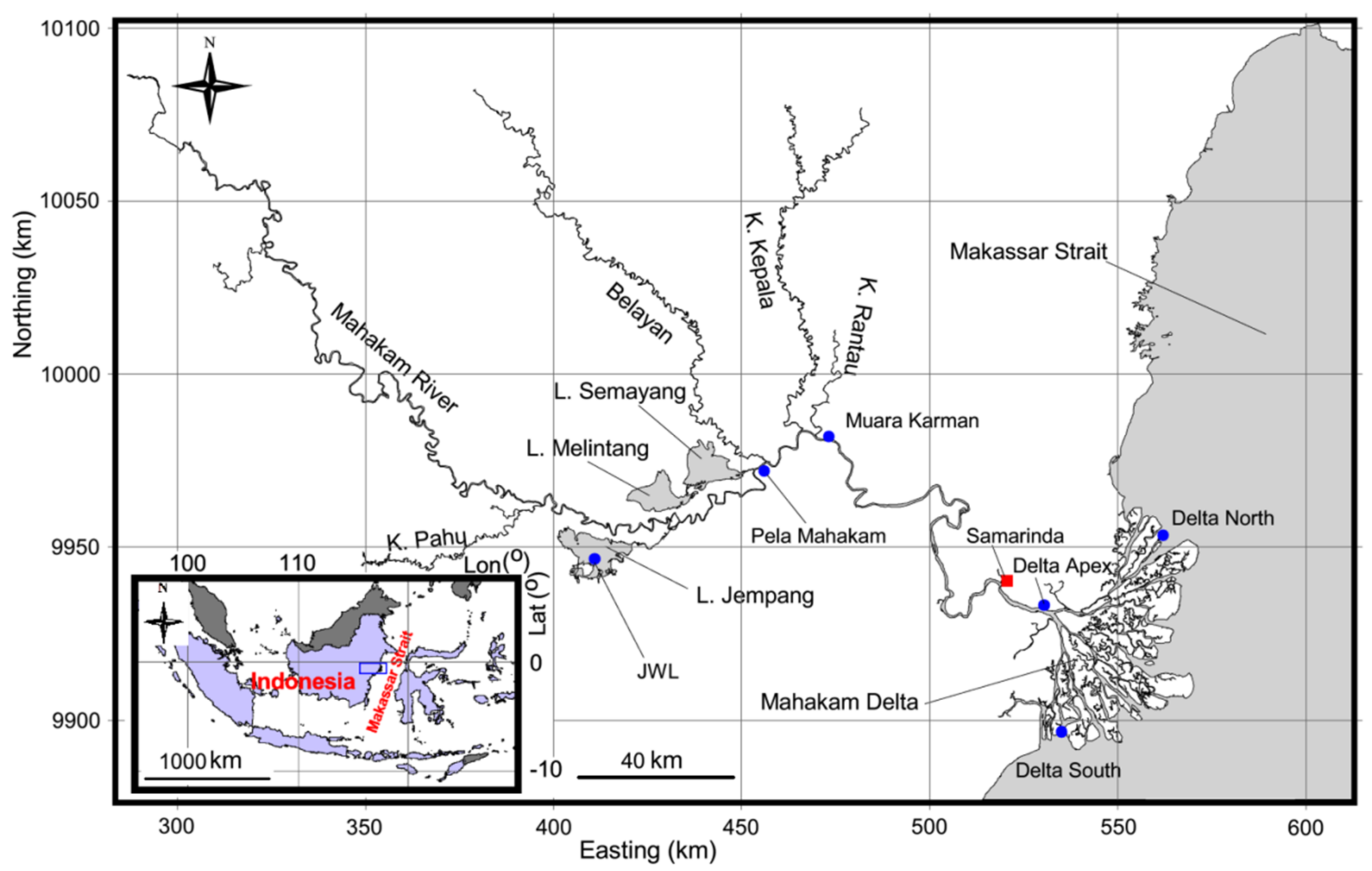
The domain of interest is the fluvial and tidal Mahakam Delta located at the mouth of the Mahakam River in the East Kalimantan province of Borneo, Indonesia (Figure 1). The delta includes a number of narrow and meandering channels. The width of the deltaic channels varies widely from 10 m to 3 km, while the depth ranges from 5 to 15 m. The delta discharges into the Makassar Strait, whose width varies between 200 and 300 km, with a length of about 600 km. Upstream of the delta is the Mahakam River, whose depth exhibits a large variability, with a maximum of the order of 45 m. The region of the river is characterized by a tropical rain forest climate with a dry season from May to September and a wet season from October to April. The river meanders over 900 km, and its catchment area covers about 75,000 km2, with a mean annual river discharge of the order of 3000 m3/s [32]. The central part of the river, located about 150 km upstream of the delta, is extremely flat. In this area, four large tributaries (Kedang Pahu, Belayan, Kedang Kepala, and Kedang Rantau) contribute greatly to the river flow, and several shallow-water lakes (e.g., Lake Jempang, Lake Melingtang, and Lake Semayang) are also connected to the river via a system of small channels. The water depth in these shallow-water lakes is of the order of 5 m.
Different activities (e.g., shrimp farming, fishing industry, transportation, and recreation [33,34]) are performed together in the Mahakam Delta, which has thus an important role in the region. However, due to the rapid developments of aquaculture activities as well as oil and gas exploitation, the deltaic environment is highly vulnerable to degradation of water quality and loss of biotopes [33]. Recent studies (e.g., [34]) found that human activities have influenced the deltaic ecosystem for many years and led to an increase of dissolved metals therein. Thus, to design measures aimed at protecting the ecosystem and achieving good water quality in the delta, it is of interest to estimate age, residence and exposure times, thereby helping understand and quantify the transport processes that carry pollutants into and out of the delta.
3. Method
3.1. Hydrodynamics Model
The Mahakam water system clearly exemplifies a continuous riverine and marine environment that includes different interconnected regions such as river, tributaries, lakes, delta, and adjacent coastal ocean. Due to the lack of field measurements of the flow and the difficulty to obtain such measurements because of the high spatial and temporal variability of the phenomena at stake, a numerical model is resorted to. It is now becoming computationally feasible to use an integrated model of the river–sea continuum without excessive simplification of the physical processes. In this context, a combined two-dimensional depth-averaged (2D) and one-dimensional section-averaged (1D) finite-element model based on SLIM (Second-generation Louvain-la-Neuve Ice-ocean Model, www.slim-ocean.be) is implemented on the Mahakam water surface system [35,36].
The version of SLIM used herein solves 1D (section-integrated) and 2D (depth-integrated) continuity, momentum, and tracer transport equations. The governing equations are discretized in space by means of the discontinuous Galerkin finite element method (DG-FEM) with linear polynomial shape functions. The time stepping relies on the second-order diagonally implicit Runge–Kutta method [37,38,39]. In order to avoid the occurrence of negative water depths, the wetting and drying algorithm designed by Kärnä et al. [39] is also implemented in the hydrodynamic model. Horizontal eddy viscosity and diffusivity are parameterized in such a way that the high mesh size variability is taken into account. The bottom stress is estimated by means of a Chézy-Manning quadratic formula. Details about the equations are provided in a previous study [36].
The 2D model is implemented in the Mahakam Delta, the adjacent Makassar Strait, and three lakes (Lake Jempang, Lake Melingtang, and Lake Semayang). On the other hand, the 1D model is used in the upstream stretch of the Mahakam River, which is 300 km in length (from the city of Melak to the delta apex) and four tributaries. Figure 2 shows the grid of the computational domain, consisting of a 2D sub-domain and a 1D sub-domain. The 2D sub-domain uses an unstructured mesh that is made of 60,819 triangular elements. The longest edge of a triangle (or mesh size) varies from 5 m in the narrowest branches of the delta to around 10 km in the deepest part of the Makassar Strait. The river and its four tributaries within the 1D sub-domain have a resolution of 100 m. The grid is generated using the open-source mesh generation software GMSH (www.geuz.org/gmsh). It must be stressed that the very complex deltaic channels and coastlines are represented in detail in the computational grid, thereby capturing most of the intricacies of the domain geometry.
As for the boundary and the initial conditions, daily water discharge is prescribed at the upstream boundaries, while tidal components (elevation and velocity harmonics) are imposed at the downstream boundaries (Figure 2). The simulation of the flow is performed for different periods of time. A six months period of high flow (from November 2008 to April 2009) and a five months period of low flow (from June to October 2009) are considered so as to investigate the transport timescales under different flow conditions. A spin up period of 30 days is applied before the beginning of each of the periods of interest. The regime conditions can be reached quickly after a few days, and thus the effects of the initial conditions can be eliminated completely. To reduce the computational time, simulation of the flow in each considered period is performed firstly, and then the hydrodynamics outputs are reloaded to calculate age, residence, and exposure times.
The hydrodynamic simulation tool applied herein to the Mahakam river–sea continuum is almost similar to that described in a previous study [36]. Therefore, it is not necessary to give additional pieces of information on this. It may, however, be appropriate to stress that a thorough calibration of the Chézy-Manning coefficient was achieved, leading to the following results: (i) a constant value of 0.023 (s/m1/3) for the Makassar Strait, (ii) a linearly increasing value in the delta region, from 0.023 (s/m1/3) in the coastal region to 0.0275 (s/m1/3) in the region from the delta front to the delta apex, (iii) a constant value of 0.0275 (s/m1/3) in the Mahakam River and its four tributaries, and (iv) a larger value of 0.0305 (s/m1/3) in the lakes.
3.2. Water Renewal Timescales
3.2.1. Age of Water
The domain of interest for timescale calculations, Ωe, is the Mahakam Delta. The water present in it consists of two components, i.e., the original water and the renewing water. The original water is the water present inside the domain at the beginning of the simulation, while the renewing water originates from the environment of the domain and progressively replaces the original water. The renewing water can enter the domain through upstream and downstream boundaries. The exact locations of the domain boundaries for timescale calculations are shown in Figure 3. The upstream boundary Γu is placed at the river mouth (i.e., the interface between the river and the delta), while the downstream boundary Γd is imposed at the delta front. According to [5], the original and the renewing waters in the delta can be treated as passive tracers and, hence, the different renewal water types can be modeled individually. If the concentrations of water originating from the upstream boundary Γu and the downstream boundary Γd of the delta are denoted Cu and Cd, respectively, the concentration of renewing water Cr in the delta, consisting of both river and sea waters, is Cr = Cu + Cd. Note that the concentration of a water type is defined as the water fraction originating from the boundary under consideration. Accordingly, these concentrations are dimensionless functions of time and position.
We assess water renewal timescales following two approaches. In the first case, we focus on the river water (i.e., from the upstream boundary of the Mahakam Delta), assuming its concentration is dominant in most of the delta. The second approach is concerned with the whole renewing water, i.e., water originating from both the upstream and the downstream boundaries.
Three water types are considered hereinafter, which are identified by subscript i (i = o, u, r). The subscripts o, u, and r refer to the original water, the renewal water from the upstream boundary, and the renewal water from both the upstream and the downstream boundaries, respectively. In the framework of CART, the age of a water type can be obtained from the solution of two advection-diffusion equations [5,17,40], which govern the depth-averaged concentration Ci and the related depth-mean age concentration αi of the water type under consideration. These equations read:
where H = η + h is the water depth, with h being the water depth below the reference level (i.e., the mean sea level), and η is the free surface elevation; u is the depth-averaged horizontal velocity vector; κ is the diffusivity coefficient that is parameterized using the Okubo formulation [41], under the form:
with ck being an appropriate constant, and Δ is the local characteristic length scale of the mesh. A value ck = 0.018 m0.85/s, which was calibrated from the best fit to the available salinity at 60 field sampling sites (see Figure 3) [42], is used to evaluate the diffusivity coefficient. The boundary and the initial conditions under which Equations (1) and (2) are to be solved are listed in Table 1. There are no concentration or age concentration fluxes through the impermeable boundaries. Finally, the age of water type i is calculated as follows [17]:
At any location in the domain of interest and at any time, the concentration and the age of each water type have to satisfy the following properties [5,40]:
Proving that inequalities and Equations (5)–(8) hold valid can be done by having recourse to demonstrations very similar to those performed in Appendices A and B of [5]. The aforementioned properties of the age suggest that the partial differential problems (from which the age of each water type and its aggregates are derived) are well posed. In other words, the behavior of the age is in accordance with physical intuition and elementary mathematical requirements.
Under the initial and the boundary conditions listed in Table 1, the concentration and the age concentration of the original water satisfy α0(t,x) = tC0(t,x), implying that the age of the original water is equal to the elapsed time, i.e., a0(t,x) = t [5,40]. This is because the original water can only leave the domain of interest as time progresses, and there is obviously no source of original water. This piece of information is of little diagnostic value. However, it is an additional element supporting the well-foundedness of the partial differential problems laid out above.
3.2.2. Residence Time
The residence time θr is defined as the time taken by a water parcel initially in the domain of interest to leave it for the first time. It can be obtained by solving, under the initial and the boundary conditions mentioned below, the partial differential equation:
It is derived from the adjoint of the equation governing the concentration of the original water [21,43]. It must be underscored that Equation (9) is not a classical depth-averaged advection–diffusion equation because of the negative sign in the diffusivity term. It must be integrated backward in time, resulting in the following equation [43]:
with τ = T − t, where T corresponds to the end of the simulation period (i.e., the time at which the reverse time integration begins).
As for the boundary condition, a no flux condition is enforced on the impermeable boundaries. According to [21], the residence time should be prescribed to be zero on the open boundaries. However, as shown in [44], a boundary layer of the residence time develops in the vicinity of the incoming open boundaries. This boundary layer cannot be resolved by the mesh employed here and hence must be treated in a suitable manner in order to prevent spurious oscillations from developing [43]. This is why it is desirable to replace the homogeneous Dirichlet boundary condition by the flux condition derived in [44] from a one-dimensional solution, which is investigated in [43]. Accordingly, the boundary conditions that are actually used in the numerical simulations are as follows:
where n is the outward normal unit vector to the boundary, un (=u.n) is the normal velocity, and L* is the width of the unresolved boundary layer. In [44], it was found to be appropriate to prescribe that the length L* be equal to the local mesh size.
The reverse time marching integration cannot be performed without prescribing an “initial” value, i.e., θr(t = T,x), which, unfortunately, is unknown. The reverse time marching is initialized with θr(t = T,x) = 0 and, after a spin up period whose duration is equal to a couple of times the typical value of the residence time, a regime solution is attained and, hence, the “initial condition” is no longer important, which is in accordance with Delhez et al. [21].
3.2.3. Exposure Time
Due the tidal motions, a water parcel that left the domain of interest Ωe at a given time can re-enter the domain many times before escaping it definitively. To account for this, the concept of exposure time is introduced, that is, the total time spent in the domain. The exposure time θe can be numerically computed by solving the following Equation [5]:
where equals 1 and 0 in and out the domain of interest Ωe, respectively.
It must be stressed that the computational domain Ω for the exposure time must be extended to explicitly represent phenomena taking place outside the domain of interest Ωe (Ωe ⊂ Ω). In the present study, the domain Ω is extended significantly both upstream and downstream of the delta, and it is taken to be identical to the computational domain used for the hydrodynamic simulations.
In the Mahakam River and four tributaries, the exposure time is obtained by solving the following one-dimensional equation:
where A is the cross-sectional area, and κ is the diffusivity coefficient. The latter is parameterized under the form of Equation (3), in which the local characteristic length scale of the grid is taken to be the distance between two channel cross-sections (i.e., 100 m). Equation (13) is also solved the same way as governing equations in the 2D sub-domain (see details in [36,42]).
A water parcel at open sea boundaries, which are located at the entrance and at the outlet of the Makassar Strait, is assumed to never return into the delta, and thus a value θe = 0 is imposed. At upstream boundaries, where the flow is assumed to be always in the downward direction, the expression κ∇θe.n = 0 is used [5]. The initial value of the exposure time is set equal to zero in the whole computational domain.
3.2.4. Finite Element Implementation
The governing equations for the age of water are solved by using a discontinuous Galerkin finite element method for the spatial operators and the second-order diagonally implicit Runge–Kutta method for the temporal operators. The computational domain is discretized into series of elements, as shown in Figure 2. The governing equations are multiplied by test functions and then integrated by parts over each element, resulting in element-wise surface and contour integral terms for the spatial operators. The surface term is solved using the DG-FEM with linear shape function, while a Roe solver is used for computing the fluxes at the interfaces between two adjacent elements in order to represent the water-wave dynamics in contour terms properly [37]. Because a second-order diagonally implicit Runge–Kutta method is employed for the temporal derivative operator [35], a time step as large as 10 min can be used for our computations. The governing equations for the residence and the exposure times are solved in a manner similar to those for the age of water. It must be kept in mind, however, that the equations for the residence and the exposure times are integrated backward in time.
The necessary hydrodynamics outputs are reloaded only in the Mahakam Delta, in the forward direction for the age simulations, and in the backward in time for the residence time simulations. The abovementioned calculation procedure is very convenient and efficient in terms of computational time. The computational procedure for the exposure time is similar to that applied for the residence time. The hydrodynamic outputs are then reloaded in the whole computational domain for the backward in time integration. Then, the exposure time is computed separately and offline with the flow dynamics in the computer procedure, as for the residence time.
4. Results and Discussion
4.1. Age of Water
4.1.1. River Water
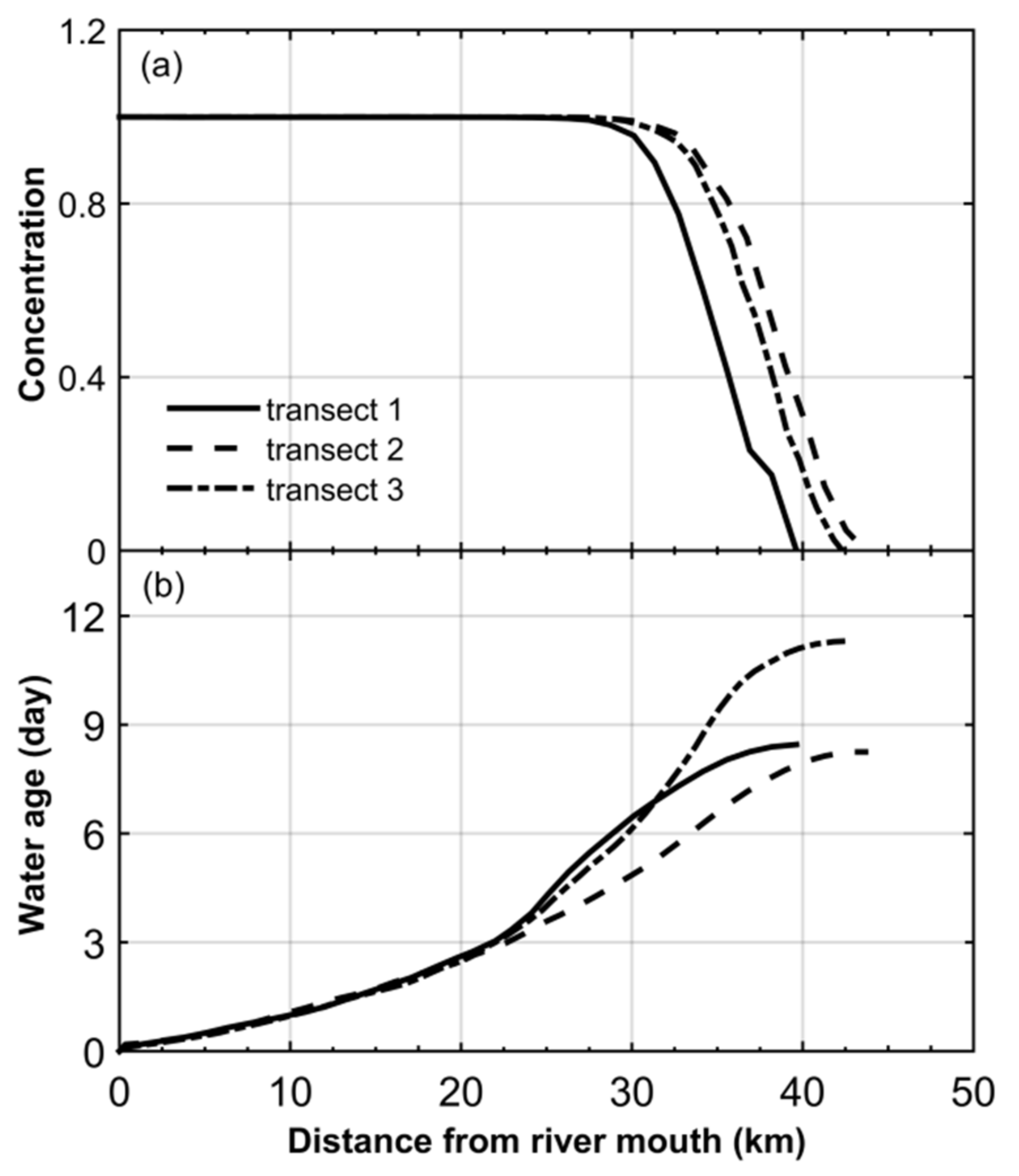
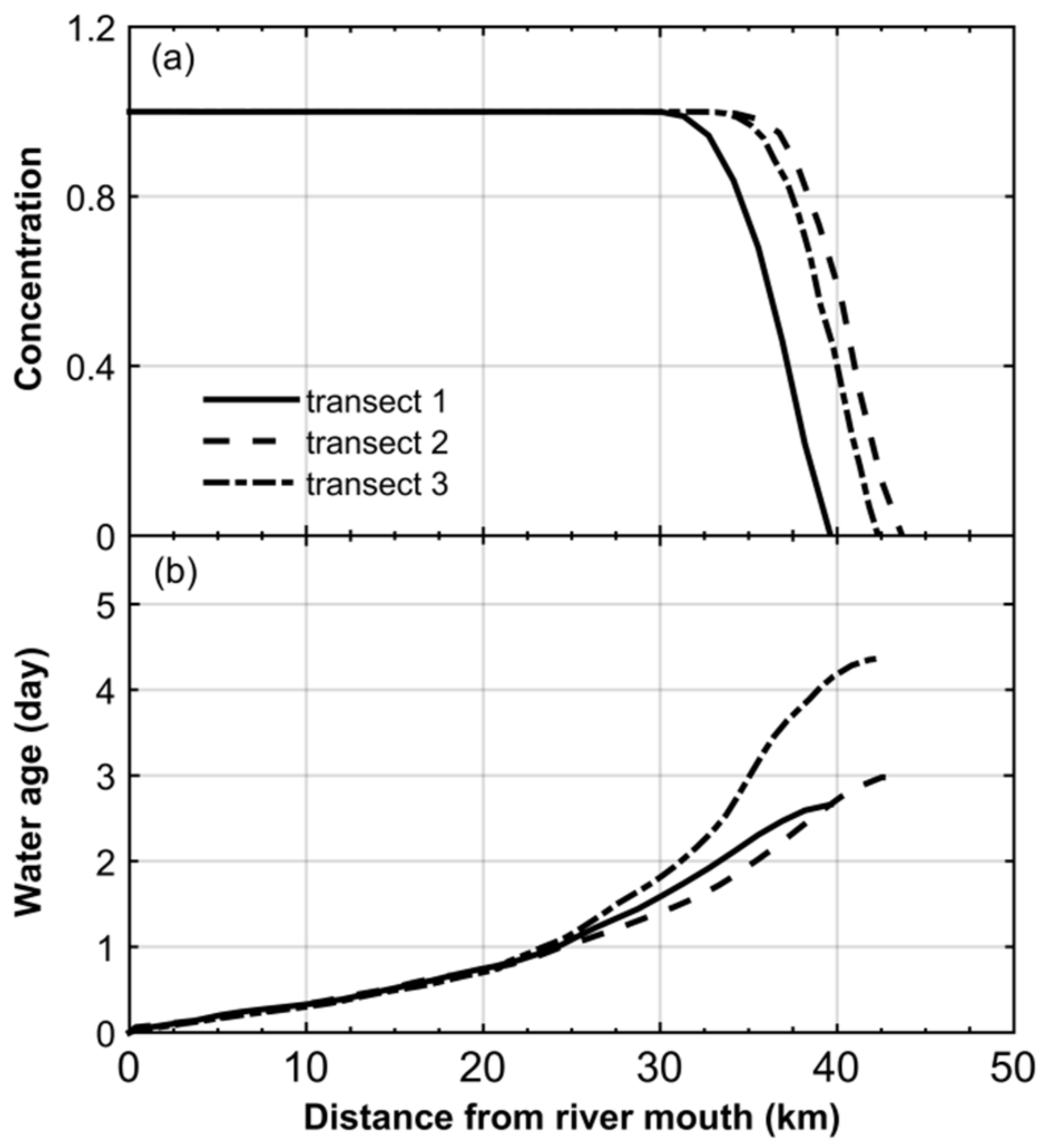
Figure 4 shows the average over the low-flow simulation period (the daily water discharge at river mouth varies from 550 to 3000 m3/s) of the concentration and the age of the river water along the three considered transects (see Figure 3). The river water concentration is equal to unity at 26 km from the river mouth (Figure 4a). Beyond this point, the concentration significantly decreases from unity to zero, resulting in a significant increase of the age of water. As shown in Figure 5a, a similar trend of the concentration is also observed for the high-flow period (during which the daily water discharge at the river mouth varies between 3500 and 6500 m3/s). The point from which the concentration begins to decrease occurs around km 31. The difference in location of the point from which the concentration starts decreasing in the low and high flow conditions can be explained by differences of water discharges.
The age of the water along the three transects monotonically increases from zero at the upstream boundary (where the river water enters the domain of interest) to a maximum value at the downstream boundary (Figure 4b). A maximum value of 9 days is obtained in the main southern and northern fluvial channels (i.e., transect 1 and transect 2), while the maximum age is about 11 days in transect 3. A nonlinear increase of the age of water from the upstream to the downstream boundaries can be explained by the decrease of the flow velocity along the transects, which is due to changes in bathymetry, channel cross-section, tidal effects, and meandering and curvature of channels [36,42]. On the other hand, to investigate the effect of the tides on the water age, the standard deviation of the water age is also calculated at each location along the three considered transects, resulting in values lying between 0.5 and 4 days. This indicates that the variation of the age of water caused by tides is about 35% of the magnitude of the averaged value in the transects.
The averaged value of the water age in the high flow period also increases from zero (at the river mouth) to 4.5 days (at the downstream boundary, Figure 5b), revealing that the magnitude of the age in the high flow is three times smaller than that in the low flow. This is due to the significant increase of the flow velocity. These results reveal that the age of water is clearly linked to the river volumetric flow rate entering the delta. The standard deviation associated with the averaged value of the age of water increases from zero to 15 h along the transects, showing that the variation of the age due to the tidal variation equals 15% of the averaged value of the age, and, as expected, tidal effects on transport processes are weaker in the high flow than in the low flow regimes.
A previous study [45] of the age of river water in the Mahakam Delta showed that the mean age over a two months simulation period (May and June 2008) varied between 4 and 7 days. Indeed, the water age ranged between zero at the delta apex and 4 days at the delta front. These results are similar to those obtained for the high flow period in the present study. The slight discrepancy may be due to differences in hydrodynamics.
On downstream boundary Γd, the concentration of the river water (Cu) and its age concentration (αu) are both prescribed to be zero, implying that the corresponding age (au = αu/Cu) is an indeterminate form, i.e., 0/0. In the absence of an analytical solution, explicitly evaluating this limit is impossible. However, this issue may be successfully addressed by first deriving the equation for the age. This is achieved by manipulating concentration and age concentration Equations (1) and (2) and casting the resulting relation into the appropriate form, eventually yielding:
On Γd, the concentration is prescribed to be zero. Therefore, Equation (14) simplifies to . In addition, since Cu is zero on Γd, its gradient is parallel to n, the unit normal vector to the boundary. As a consequence, the age satisfies boundary condition , i.e., the derivative of the age in the direction normal to the boundary must be zero, which is why the age should have a finite value on the boundary. To the best of our knowledge, this theoretical result is novel. The simulated age profiles displayed on Figure 4 and Figure 5 are in agreement with it.
4.1.2. Total Renewing Water
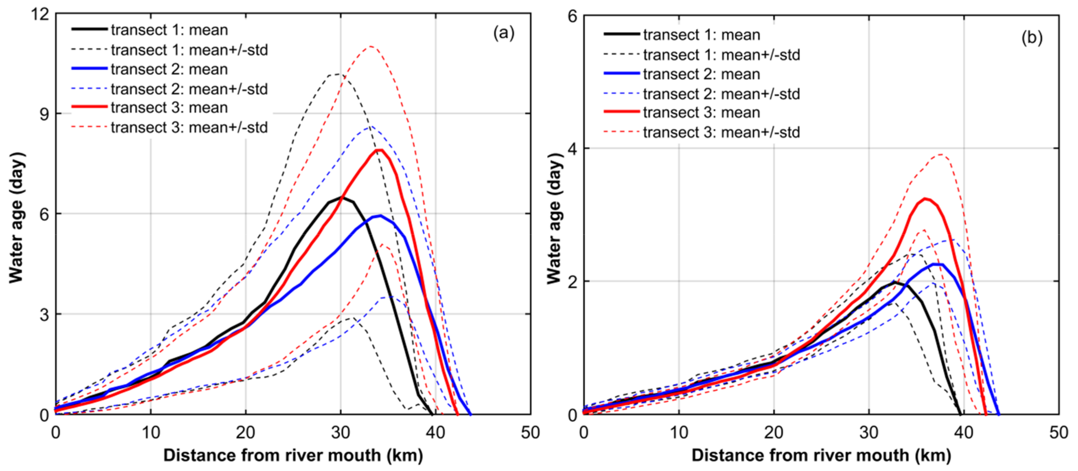
Figure 6 shows the age of the total renewing water. The total renewing water concentration along the three considered transects equals unity for both the high and the low flow periods because once the transient solution has vanished, all the original water is replaced by renewing water. As shown in Figure 6a for the low flow period, the averaged values of the total renewing water age along the transects increase from zero at boundaries to a maximum value at km 34 (as measured from the river mouth). The maximum values are 7, 6, and 8.5 days in transects 1, 2, and 3, respectively. The variation of the age of water caused by the tide along the transects ranges from 0 to 4 days, especially from km 20 to the downstream boundaries.
Figure 6b shows the age of water obtained in the high flow period. The age increases from zero at the boundaries to peak values (i.e., 2.0, 2.3, and 3.2 days in the transects 1, 2, and 3). The peak of the age in the high flow period is smaller by a factor of two to three than that in the low flow period, indicating again that the age of the total renewing water is also clearly linked to the water discharge entering the delta. The location of the peak value moves slightly in the seaward direction, around km 36. The standard deviation associated with mean age along the three considered transects is less than 1 day.
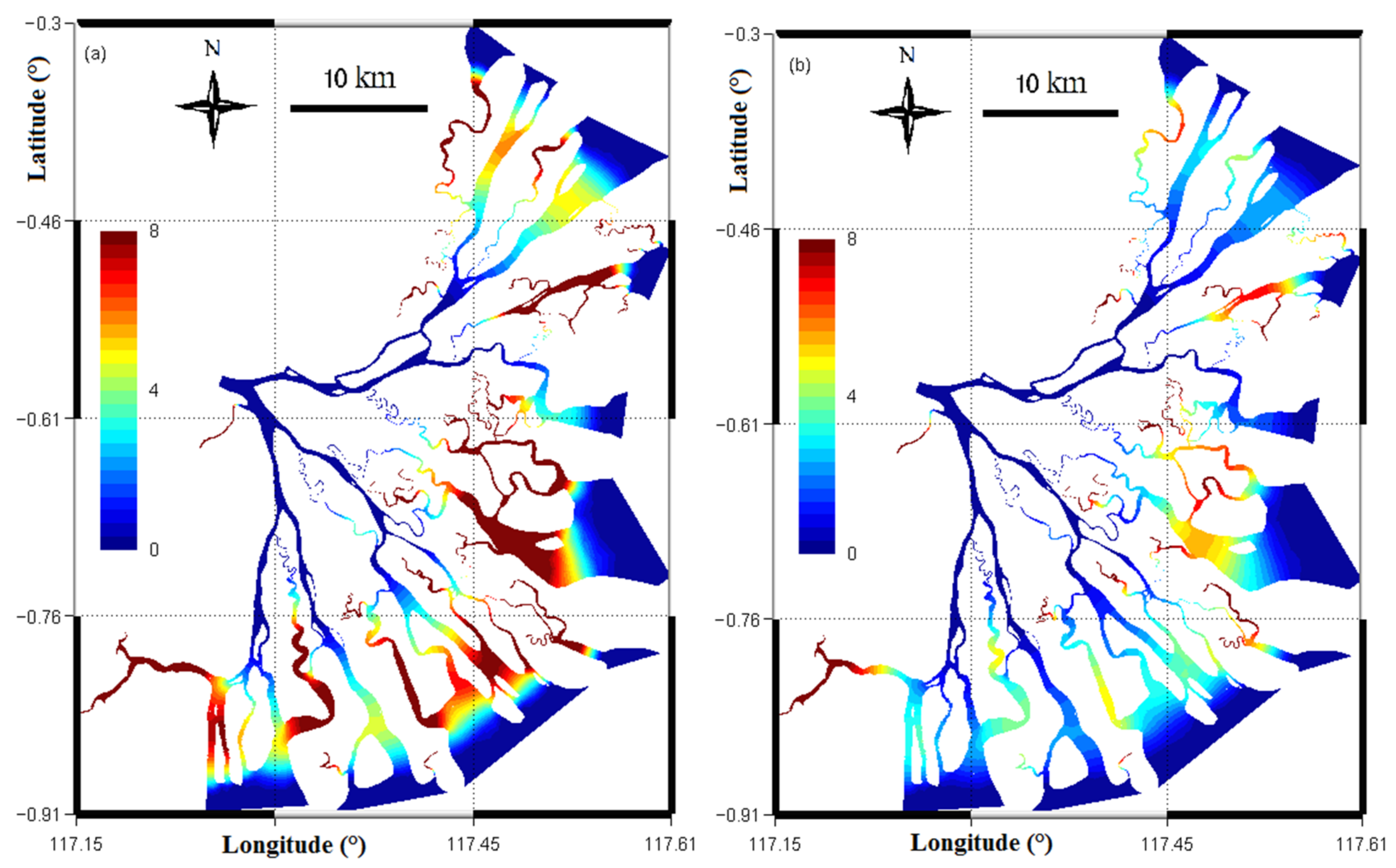
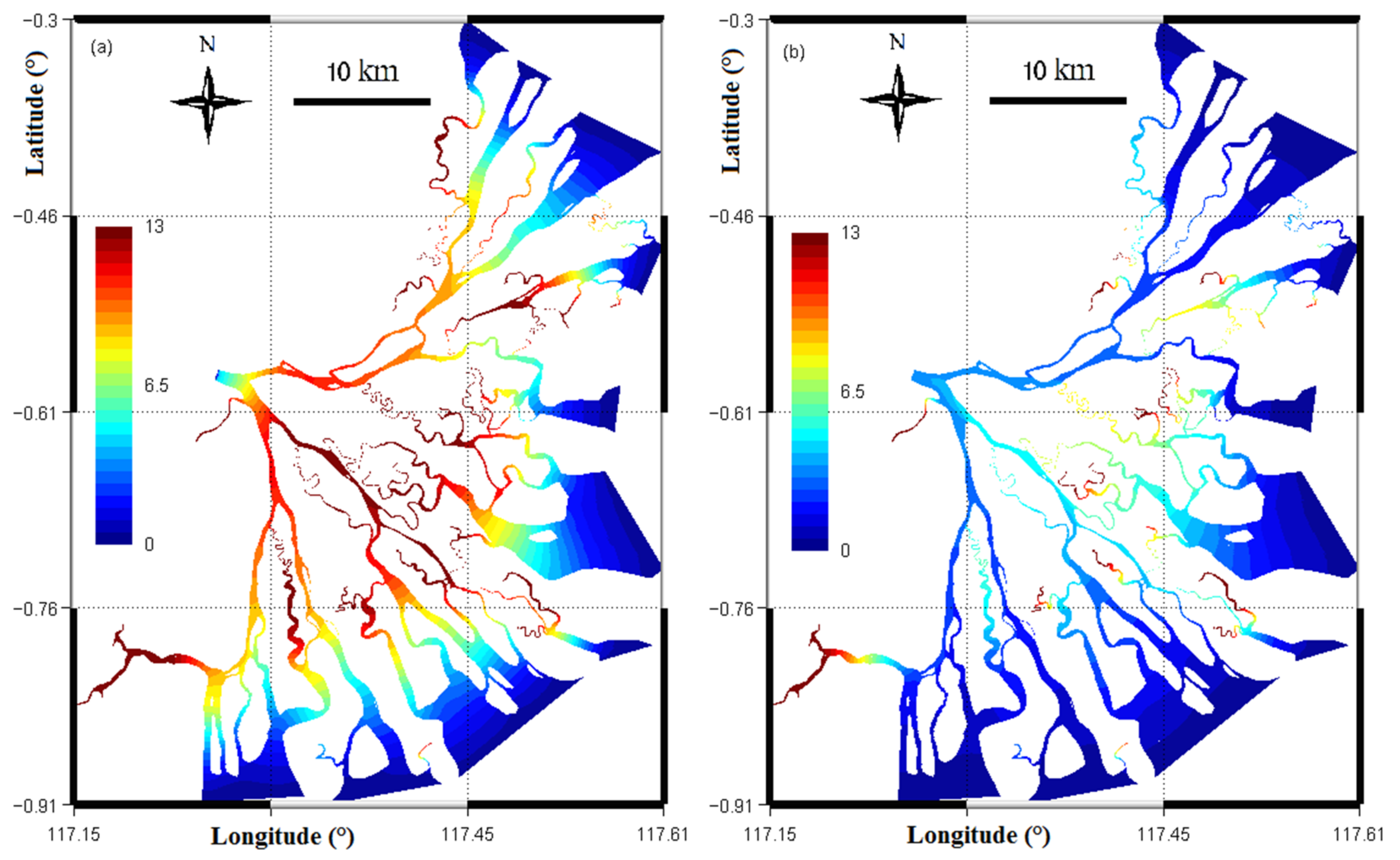
Figure 7a shows the spatial distribution of the averaged value of the water age for the low flow period. The mean age varies significantly in space, depending on locations and channels in the delta. The age is generally large in the middle region of the delta, where the complex hydrodynamics is caused by the combined effect of tide, river flow, and rugged geometry. A maximum value of 20 days is found in several small and narrow deltaic channels and in the creeks.
The distribution of the averaged value of the water age for the high flow period is shown in Figure 7b. Similarly to the low flow period, the mean age also varies significantly in the deltaic region. A small value of the age (e.g., 2 days) generally occurs in the fluvial channels, e.g., transect 1, transect 2, while a larger value appears in the fluvial-tidal channels (e.g., transect 3) as well as in the creeks. The largest value of the age of water is about 15 days in the isolated tidal channels and in the creeks of the delta. This complex spatial distribution of the age mainly reflects the complex hydrodynamics, the influence of the tides, and the division of water discharge in deltaic channels. The age in the high flow period is two to three times smaller than that obtained in the low flow period.
4.2. Residence Time
The residence time must be zero on both the upstream and the downstream boundaries. However, the thin boundary layer adjacent to the incoming boundaries cannot be resolved by the present model grid, which is precisely why boundary condition (Equation (11)) is implemented. This important fact must be kept in mind when inspecting and interpreting the figures related to the residence time.
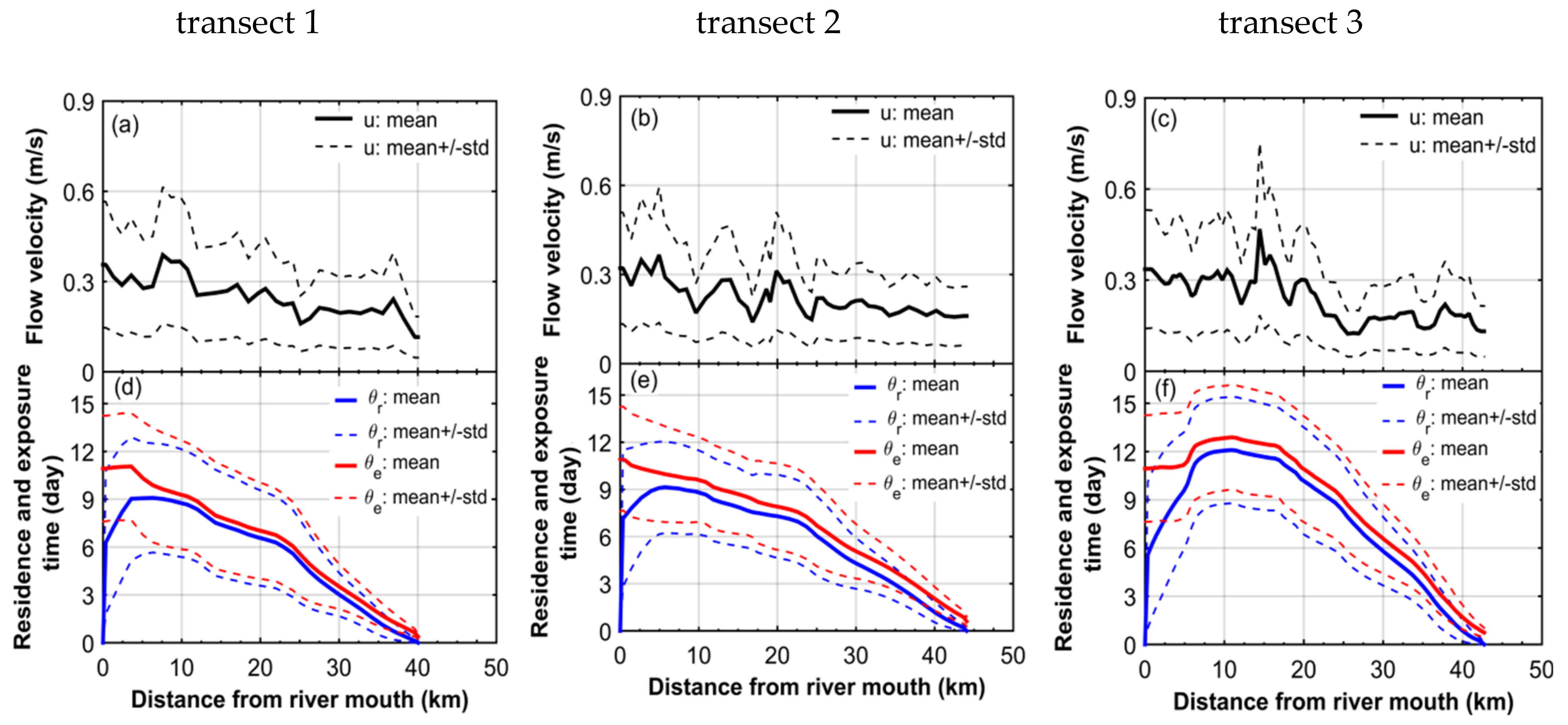
Simulated values of the residence time over the whole period of the low flow regime are shown in Figure 8 for the three considered transects, indicating that the averaged value of residence time varies in a range between 0 and 9 days in transects 1 and 2. A wider range of the residence time, from 0 to 12 days, is obtained in transect 3. The standard deviation of the averaged value of the residence time varies between zero and 3.5 days along these transects.
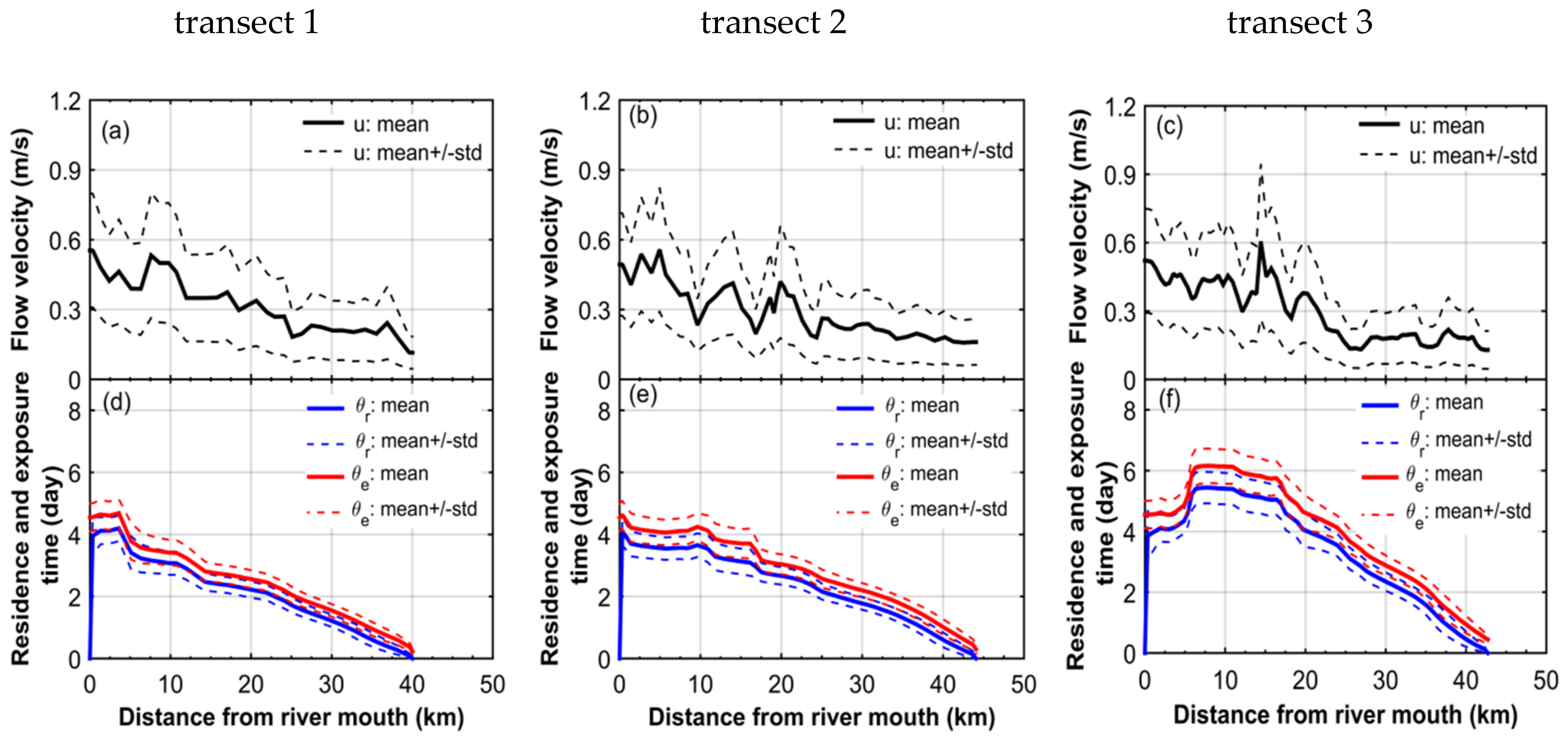
Figure 9 shows the averaged values of the residence time over the high flow period. The residence time generally decreases from the upstream to the downstream boundary. In the main southern and northern fluvial channels, a water parcel initially located at the delta apex takes, on average, about 4 days to leave the delta. In the meandering fluvial-tidal channel (i.e., transect 3), the water parcel spends a longer time (about 5.3 days) to leave the domain of interest, except at a distance of 5 km from the river mouth. The averaged value of the residence time in the high flow condition is two times smaller than that in the low flow conditions. The residence time standard deviation is more or less 20 h in all considered transects. As illustrated by Figure 10, part of the time variation of the residence time is caused by tides. The starting instant within a tidal cycle has a significant impact on the residence time despite the fact that the duration of a tidal cycle is significantly smaller than the order of magnitude of the residence time. A similar behavior of the residence time has been simulated in other estuaries [5,46]. Unfortunately, this intriguing property has yet to be fully explained.
In each transect, the residence time does not monotonically decrease with the distance in the seaward direction for either the low or the high flow periods. The variation of the residence time coincides with the changes of the longitudinal velocity (see Figure 8a–c and Figure 9a–c). This result confirms again that the residence time is a useful measure of the influence of the flow dynamics on transport processes [21].
In transect 3, the residence time increases up to a peak value of 12 days for the low flow regime (see Figure 8b) and 5.3 days for the high flow one (Figure 9b) in the first few kilometers downstream of the river mouth. The reason for this variation of the residence time can be explained by the decrease of water discharge resulting from channel bifurcations. Downstream of the delta apex bifurcation (the bifurcation right after the river mouth), only about 40% of water discharge flows into transect 2, while 60% of water discharge continuously flows in the main southern channel, i.e., transect 1 [45]. Similarly, beyond the first bifurcation in the transect 1, about 33% of water discharge in transect 1 continuously flows in the transect 3.
Figure 11 depicts the spatial distribution of the averaged value of the residence time for the low flow (Figure 11a) and for the high flow one (Figure 11b). The residence time varies significantly in space due to the changes of bathymetry and related hydrodynamics features. For instance, water parcels in tidal channels and in the creeks within the middle area of the delta take a longer time to leave the delta than water parcels in the main fluvial channels (e.g., southern and northern channels). This is because, in these channels and creeks, the water velocity is rather low. The residence time in the whole delta ranges from 0 to 15 days for both high and low flows, presenting a slightly wider range of variation in comparison with that of the water age.
The Mahakam Delta is dominated by the mangrove ecosystem, with water containing many phytoplankton species [47,48], i.e., the basic component of the food chain that is expressed by chlorophyll concentration. Previous studies [23,49] suggest that, among different factors (e.g., nutrients, residence time, geomorphological features), the chlorophyll concentration has the highest correlation with the residence time, especially in regions where the residence time is below 50 days [23]. Indeed, phytoplankton biomass is controlled by the residence time more than by nutrient availability. As for the Mahakam Delta, study of phytoplankton and of relations between chlorophyll concentration and the residence time is relatively limited. The current simulation results of the residence time are believed to be helpful for investigating the phytoplankton in the next stages of the research.
4.3. Exposure Time
Figure 8c and Figure 9c show the estimated exposure time along the three considered transects for the high and the low flow periods. The spatial distribution of the exposure time in the whole delta is shown in Figure 12, revealing that the exposure time is extremely different in the different periods. In comparison with the residence time, the estimated exposure time clearly depicts two different aspects. Firstly, the exposure time at the upstream and the downstream boundaries of the delta is far from zero, indicating that the model is able to capture the reentering of water parcels caused by tidal variations. Secondly, the exposure time is always larger than the residence time in most deltaic channels, except in small creeks located in the middle delta, in which the exposure time is more or less identical to the residence time. The standard deviation of the exposure time under tidal variation in deltaic channels is similar to that of the residence time.
4.4. Return Coefficient
The relative difference between the exposure and the residence time is often represented with the help of the return coefficient (rc) [5,26,46], which is computed as:
where θe and θr are exposure and residence time, respectively. According to this definition, the return coefficient varies between zero and one. The lower limit of the return coefficient (rc = 0) occurs when the exposure time equals the residence time or when no water parcels re-enters the delta. In contrast, the upper limit of the return coefficient (rc = 1) is reached if the residence time is much smaller than the exposure time.
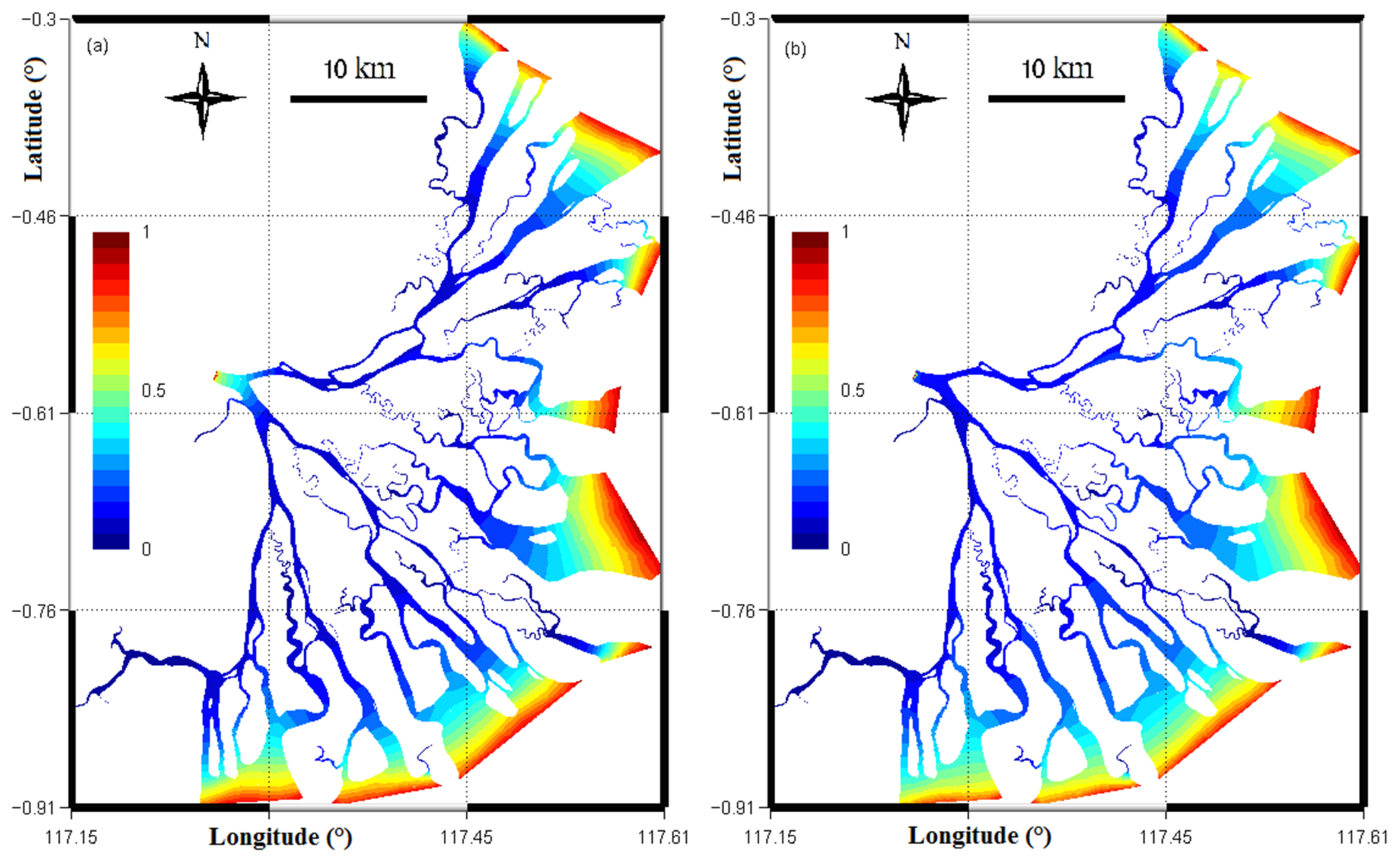
Figure 13 shows the spatial distribution of the return coefficient for the period of the low flow (Figure 13a) and for the period of the high flow (Figure 13b). The return coefficient value is averaged over each considered period. There is a slight difference of the return coefficient in different flow conditions. The return coefficient equals to unity on the upstream and the downstream boundaries, as it should be. In the middle region of the delta, the return coefficient is around 0.3, suggesting that, even far away from the open boundaries, the impact of the re-entering is non negligible.
5. Conclusions
The Mahakam Delta presents a complex geometry and topography, with complicated flow and transport processes caused by the influence of both riverine and marine forcings. The aims of this study were to assess water renewal rates under low and high flow conditions. The results clearly showed that, firstly, there was a clear link between water renewal timescales and the river volumetric flow rate. In the main deltaic channels, the age of the renewing water from the upstream delta and the age of renewing water from both the upstream and the downstream of the delta were respectively 5 and 3.5 days for the high flow, while these values were generally three times greater in the low flow. The residence and the exposure times were 6 days in the high flow and about 12 days in the low flows. The magnitude of the three water renewal timescales under different flow conditions is of the order of one spring-neap tidal cycle in the whole delta.
Secondly, the age of renewing water from the upstream delta monotonically increased from the river mouth to the delta front, while the age of renewing water from both the upstream and the downstream of the delta monotonically increased from the river mouth and the delta front to the middle delta. The residence and the exposure times did not decrease monotonically with the distance in the seaward direction, and variations of these timescales coincided with the changes of the flow velocity, revealing that these timescales are more sensitive to the change of flow dynamic than the age.
Thirdly, along deltaic channels, the variation of the water renewal timescales caused by the tide was about 35% of the order of magnitude of the averaged value. The results also clearly showed that the model was able to capture the reentering of water parcels caused by tidal variations, e.g., return coefficient was close to unity at the delta apex and delta front, while its value was about 0.3 in the middle region of the delta.
Author Contributions
Conceptualization: C.P.V., B.d.B., A.d.B., A.J.F.(T.)H., S.S.-F., E.D.; methodology: E.D.; software: C.P.V., B.d.B.; formal analysis: C.P.V., B.d.B., A.d.B., E.D.; writing—original draft preparation: C.P.V., E.D.; writing—review and editing: C.P.V., B.d.B., A.d.B., A.J.F.(T.)H., S.S.-F., E.D.; visualization: C.P.V., B.d.B.; Funding acquisition: S.S.-F., E.D. All authors have read and agreed to the published version of the manuscript.
Funding
This research received no external funding.
Acknowledgments
Eric Deleersnijder and Sandra Soares-Frazão are honorary research associates with the Belgium Fund for Scientific Research (F.R.S.—FNRS). C.P.V. and E.D. are indebted to Insaf Draoui for her useful comments on an early version of the manuscript.
Conflicts of Interest
The authors declare no conflict of interest.
References
- Jay, D.A.; Greyer, W.R.; Montgomery, D.R. An ecological perpective on estuarine classification. In A Synthetic Approach to Research and Practice; Island Press: Washington, DC, USA, 2000; pp. 149–175. [Google Scholar]
- Halpern, B.S.; Walbridge, S.; Selkoe, K.A.; Kappel, C.V.; Micheli, F.; D’Agrosa, C.; Bruno, J.F.; Casey, K.S.; Ebert, C.; Fox, H.E.; et al. A Global Map of Human Impact on Marine Ecosystems. Science 2008, 319, 948–952. [Google Scholar] [CrossRef] [PubMed] [Green Version]
- Shi, H.; Yu, X. Application of transport timescales to coastal environmental assessment: A case study. J. Environ. Manag. 2013, 130, 176–184. [Google Scholar] [CrossRef] [PubMed]
- Monsen, N.; Cloern, J.; Lucas, L.; Monismith, S. A comment on the use of flushing time, residence time, and age as transport time scales. Limnol. Oceanogr. 2002, 47, 1545–1553. [Google Scholar] [CrossRef] [Green Version]
- De Brye, B.; De Brauwere, A.; Gourgue, O.; Delhez, E.J.M.; Deleersnijder, E. Water renewal timescales in the Scheldt Estuary. J. Mar. Syst. 2012, 94, 74–86. [Google Scholar] [CrossRef]
- Viero, D.P.; Defina, A. Water age, exposure time, and local flushing time in semienclosed, tidal basins with negligible freshwater inflow. J. Mar. Syst. 2016, 156, 16–29. [Google Scholar] [CrossRef]
- Bolin, B.; Rodhe, H. A note on the concepts of age distribution and transit time in natural reservoirs. Tellus 1973, 25, 58–62. [Google Scholar] [CrossRef]
- Zimmerman, J.T.F. Mixing and flushing of tidal embayments in the western Dutch wadden sea part I: Distribution of salinity and calculation of mixing time scales. Neth. J. Sea Res. 1976, 10, 149–191. [Google Scholar] [CrossRef]
- Huang, W.; Liu, X.; Chen, X.; Flannery, M.S. Estimating river flow effects on water ages by hydrodynamic modeling in Little Manatee River estuary, Florida, USA. Environ. Fluid Mech. 2010, 10, 197–211. [Google Scholar] [CrossRef]
- Gross, E.; Andrews, S.; Bergamaschi, B.; Downing, B.; Holleman, R.; Burdick, S.; Durand, J. The use of stable isotope-based water age to evaluate a hydrodynamic model. Water 2019, 11, 2207. [Google Scholar] [CrossRef] [Green Version]
- Takeoka, H. Fundamental concepts of exchange and transport time scales in a coastal sea. Cont. Shelf Res. 1984, 3, 311–326. [Google Scholar] [CrossRef]
- Liu, W.-C.; Chen, W.-B.; Kuo, J.-T.; Wu, C. Numerical determination of residence time and age in a partially mixed estuary using three-dimensional hydrodynamic model. Cont. Shelf Res. 2008, 28, 1068–1088. [Google Scholar] [CrossRef]
- Ren, Y.; Lin, B.; Sun, J.; Pan, S. Predicting water age distribution in the Pearl River Estuary using a three-dimensional model. J. Mar. Syst. 2014, 139, 276–287. [Google Scholar] [CrossRef]
- Kärnä, T.; Baptista, A.M. Water age in the Columbia River estuary. Estuar. Coast. Shelf Sci. 2016, 183, 249–259. [Google Scholar] [CrossRef] [Green Version]
- Yang, J.; Kong, J.; Tao, J. Modeling the water-flushing properties of the Yangtze estuary and adjacent waters. J. Ocean Univ. China 2019, 18, 93–107. [Google Scholar] [CrossRef]
- Shang, J.; Sun, J.; Tao, L.; Li, Y.; Nie, Z.; Liu, H.; Chen, R.; Yuan, D. Combined effect of tides and wind on water exchange in a semi-enclosed shallow sea. Water 2019, 11, 1762. [Google Scholar] [CrossRef] [Green Version]
- Deleersnijder, E.; Campin, J.-M.; Delhez, E.J.M. The concept of age in marine modelling I. Theory and preliminary model results. J. Mar. Syst. 2001, 28, 229–267. [Google Scholar] [CrossRef] [Green Version]
- De Serio, F.; Armenio, E.; Ben Meftah, M.; Capasso, G.; Corbelli, V.; De Padova, D.; De Pascalis, F.; Di Bernardino, A.; Leuzzi, G.; Monti, P.; et al. Detecting sensitive areas in confined shallow basins. Environ. Model. Softw. 2020, 126, 104659. [Google Scholar] [CrossRef]
- Braunschweig, F.; Martins, F.; Chambel, P.; Neves, R. A methodology to estimate renewal time scales in estuaries: The Tagus Estuary case. Ocean Dyn. 2003, 53, 137–145. [Google Scholar] [CrossRef]
- Shen, J.; Haas, L. Calculating age and residence time in the tidal York River using three-dimensional model experiments. Estuar. Coast. Shelf Sci. 2004, 61, 449–461. [Google Scholar] [CrossRef]
- Delhez, E.J.M.; Heemink, A.W.; Deleersnijder, E. Residence time in a semi-enclosed domain from the solution of an adjoint problem. Estuar. Coast. Shelf Sci. 2004, 61, 691–702. [Google Scholar] [CrossRef]
- Cloern, J.E.; Cole, B.E.; Wong, R.L.J.; Alpine, A.E. Temporal dynamics of estuarine phytoplankton: A case study of San Francisco Bay. Hydrobiologia 1985, 129, 153–176. [Google Scholar] [CrossRef]
- Delesalle, B.; Sournia, A. Residence time of water and phytoplankton biomass in coral reef lagoons. Cont. Shelf Res. 1992, 12, 939–949. [Google Scholar] [CrossRef]
- Lucas, L.; Thompson, J.; Brown, L. Why are diverse relationships observed between phytoplankton biomass and transport time? Limnol. Oceanogr. 2009, 54, 381–390. [Google Scholar] [CrossRef]
- Arega, F.; Armstrong, S.; Badr, A.W. Modeling of residence time in the East Scott Creek Estuary, South Carolina, USA. J. Hydro-Environ. Res. 2008, 2, 99–108. [Google Scholar] [CrossRef]
- De Brauwere, A.; De Brye, B.; Blaise, S.; Deleersnijder, E. Residence time, exposure time and connectivity in the Scheldt Estuary. J. Mar. Syst. 2011, 84, 85–95. [Google Scholar] [CrossRef]
- Andutta, F.P.; Ridd, P.V.; Deleersnijder, E.; Prandle, D. Contaminant exchange rates in estuaries—New formulae accounting for advection and dispersion. Prog. Oceanogr. 2014, 120, 139–153. [Google Scholar] [CrossRef] [Green Version]
- Huguet, J.R.; Brenon, I.; Coulombier, T. Characterisation of the water renewal in a macro-tidal Marina using several transport timescales. Water 2019, 11, 2050. [Google Scholar] [CrossRef] [Green Version]
- Cheng, Y.; Mu, Z.; Wang, H.; Zhao, F.; Li, Y.; Lin, L. Water residence time in a typical tributary bay of Three Corges reservoir. Water 2019, 11, 1585. [Google Scholar] [CrossRef] [Green Version]
- Lovecchio, S.; Marchioli, C.; Soldati, A. Time persistency of floating particle clusters in free-surface turbulence. Phys. Rev. E 2013, 88, 033003. [Google Scholar] [CrossRef] [Green Version]
- Gutiérrez, P.; Aumaitre, S. Clustering of floaters on the free surface of a turbulent flow: An experimental study. Eur. J. Mech. B/Fluids 2016, 60, 24–32. [Google Scholar] [CrossRef] [Green Version]
- Allen, G.P.; Chambers, J.L.C. Sedimentation in the Modern and Miocene Mahakam Delta; Indonesian Petroleum Association: Jakarta, Indonesia, 1998; p. 236. Available online: https://books.google.be/books?id=2j9OAQAAIAAJ (accessed on 1 January 1998).
- Chaîneau, C.-H.; Mine, J.; Suripno. The integration of biodiversity conservation with oiland gas exploration in sensitive tropical environments. Biodivers. Conserv. 2010, 19, 587–600. [Google Scholar] [CrossRef]
- Budiyanto, F. Study of metal contaminant level in the Mahakam Delta: Sediment and dissolved metal perpectives. J. Coast. Dev. 2013, 16, 147–157. [Google Scholar]
- De Brye, B. Multiscale Finite-Element Modelling of River-Sea Continua. Ph.D. Thesis, Université Catholique de Louvain, Louvain-la-Neuve, Belgium, 2011. [Google Scholar]
- Pham Van, C.; De Brye, B.; Spinewine, B.; Deleersnijder, E.; Hoitink, A.J.F.; Sassi, M.G.; Hidayat, H.; Soares-Frazão, S. Simulations of flow in the tropical river-lake-delta system of the Mahakam land-sea continuum, Indonesia. Environ. Fluid Mech. 2016, 16, 603–633. [Google Scholar] [CrossRef] [Green Version]
- Comblen, R.; Lambrechts, J.; Remacle, J.-F.; Legat, V. Practical evaluation of five partly discontinuous finite element pairs for the non-conservative shallow water equations. Int. J. Numer. Methods Fluids 2010, 63, 701–724. [Google Scholar] [CrossRef]
- De Brye, B.; De Brauwere, A.; Gourgue, O.; Kärnä, T.; Lambrechts, J.; Comblen, R.; Deleersnijder, E. A finite-element, multi-scale model of the Scheldt tributaries, river, estuary and ROFI. Coast. Eng. 2010, 57, 850–863. [Google Scholar] [CrossRef]
- Kärnä, T.; De Brye, B.; Gourgue, O.; Lambrechts, J.; Comblen, R.; Legat, V.; Deleersnijder, E. A fully implicit wetting-drying method for DG-FEM shallow water models, with an application to the Scheldt Estuary. Comput. Methods Appl. Mech. Eng. 2011, 200, 509–524. [Google Scholar] [CrossRef]
- Gourgue, O.; Deleersnijder, E.; White, L. Toward a generic method for studying water renewal, with application to the epilimnion of Lake Tanganyika. Estuar. Coast. Shelf Sci. 2007, 74, 628–640. [Google Scholar] [CrossRef]
- Okubo, A. Oceanic diffusion diagrams. Deep Sea Res. 1971, 18, 789–802. [Google Scholar] [CrossRef]
- Pham Van, C.; Gourgue, O.; Sassi, M.; Deleersnijder, E.; Hoitink, A.J.F.; Soares-Frazao, S. Modelling fine-grained sediment transport in the Mahakam land-sea continuum, Indonesia. J. Hydro-Environ. Res. 2016, 13, 103–120. [Google Scholar] [CrossRef] [Green Version]
- Blaise, S.; De Brye, B.; De Brauwere, A.; Deleersijder, E.; Delhez, E.J.M.; Comblen, R. Capturing the residence time boundary layer—Application to the Scheldt Estuary. Ocean Dyn. 2010, 60, 535–554. [Google Scholar] [CrossRef]
- Delhez, E.J.M.; Deleersnijder, E. The boundary layer of the residence time field. Ocean Dyn. 2006, 56, 139–150. [Google Scholar] [CrossRef]
- De Brye, B.; Schellen, S.; Sassi, M.; Vermeulen, B.; Karna, T.; Deleersijder, E.; Hoitink, T. Preliminary results of a finite-element, multi-scale model of the Mahakam Delta (Indonesia). Ocean Dyn. 2011, 61, 1107–1120. [Google Scholar] [CrossRef]
- Andutta, F.P.; Helfer, F.; De Miranda, L.B.; Deleersnijder, E.; Thomas, C.; Lemckert, C. An assessment of transport timescales and return coefficient in adjacent tropical estuaries. Cont. Shelf Res. 2016, 124, 49–62. [Google Scholar] [CrossRef] [Green Version]
- Budhiman, S.; Salama, S.M.; Vekerdy, Z.; Verhoef, W. Deriving optical properties of Mahakam Delta coastal waters, Indonesia using in situ measurements and ocean color model inversion. ISPRS J. Photogramm. Remote Sens. 2012, 68, 157–169. [Google Scholar] [CrossRef]
- Suroso, B.; Hutabarat, J.; Afiati, N. The Potential of Tiger Prawn Fry from Delta Mahakam, East Kalimantan Indonesia. Int. J. Sci. Eng. 2013, 6, 43–46. [Google Scholar] [CrossRef] [Green Version]
- Furnas, M.J.; Mitchell, A.W.; Gilmartin, M.; Revelante, N. Phytoplantonk biomass and primary production in semi-enclosed reef lagoons of the central Great Barrier Reef, Australia. Coral Reefs 1990, 9, 1–10. [Google Scholar] [CrossRef]
Figure 1.
Map of the Mahakam river system and delta channel network, Borneo Island, Indonesia.

Figure 2.
Grid of the computational domain: (a) whole computational mesh and (b) zoom on upstream domain and delta, showing the connection between the 1D and the 2D sub-domains (dashed-blue lines) and upstream boundary locations (black dots).
Figure 2.
Grid of the computational domain: (a) whole computational mesh and (b) zoom on upstream domain and delta, showing the connection between the 1D and the 2D sub-domains (dashed-blue lines) and upstream boundary locations (black dots).

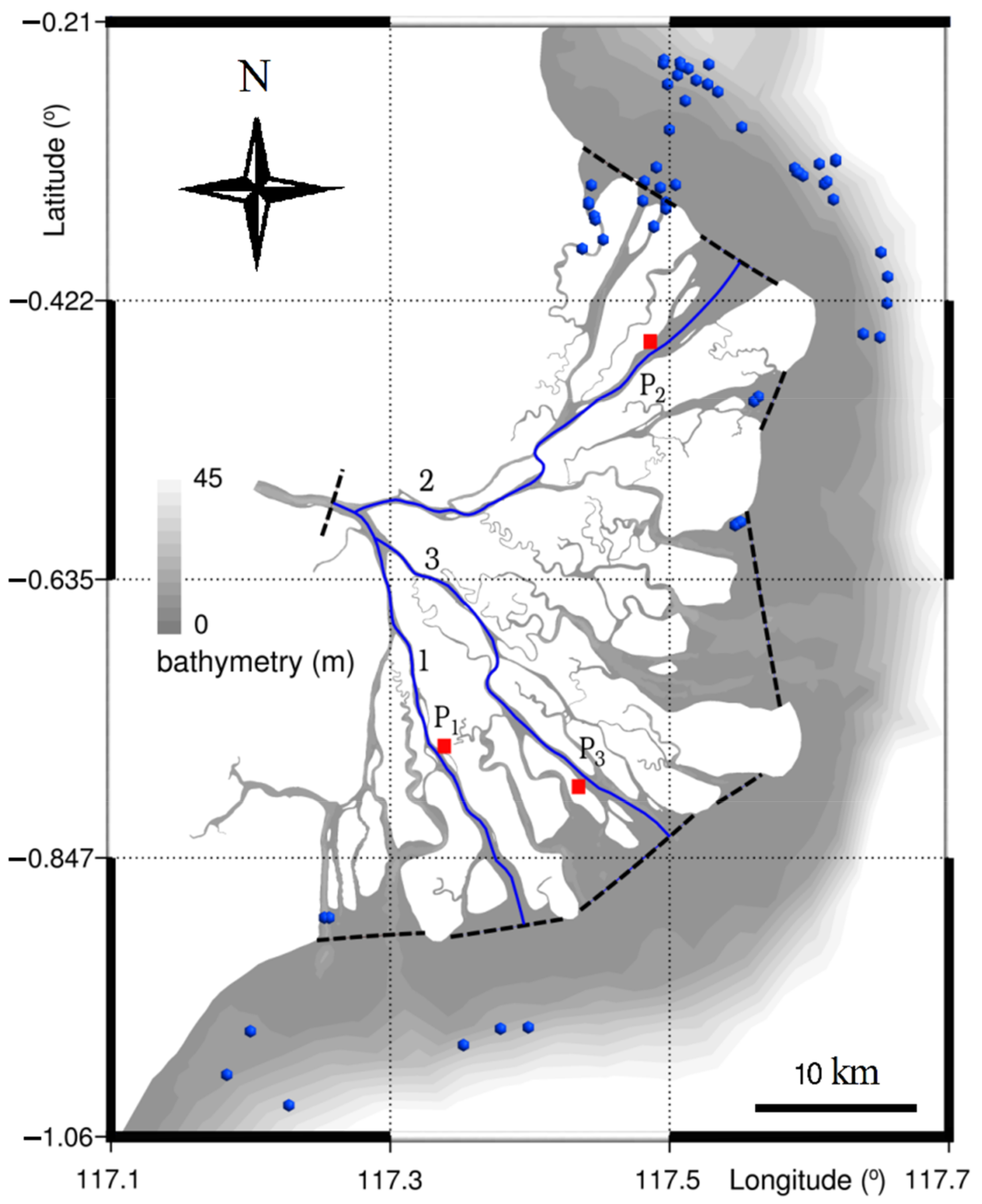
Figure 3.
Bathymetry in the delta and the delta front, with field sampling sites of salinity (blue dots), upstream and downstream boundaries (black dashed lines) for computing the water renewal timescales, the three considered transects (blue lines) and three points (red squares).
Figure 3.
Bathymetry in the delta and the delta front, with field sampling sites of salinity (blue dots), upstream and downstream boundaries (black dashed lines) for computing the water renewal timescales, the three considered transects (blue lines) and three points (red squares).

Figure 4.
Calculation results of: (a) concentration and (b) water age during the low flow period, along the three considered transects (see Figure 3) for the case of the river water.
Figure 4.
Calculation results of: (a) concentration and (b) water age during the low flow period, along the three considered transects (see Figure 3) for the case of the river water.

Figure 5.
Calculation results of: (a) concentration and (b) water age during the high flow period, along the three considered transects (see Figure 3) for the case of the river water.
Figure 5.
Calculation results of: (a) concentration and (b) water age during the high flow period, along the three considered transects (see Figure 3) for the case of the river water.

Figure 6.
Calculation results of the age of the total renewing water during the: (a) low flow period and (b) high flow period, along the three considered transects (see Figure 3).
Figure 6.
Calculation results of the age of the total renewing water during the: (a) low flow period and (b) high flow period, along the three considered transects (see Figure 3).

Figure 7.
Distribution of the age of the total renewing water for the: (a) low and (b) high flow period. The color bar is cropped at 8 days in order to focus on the variation of the age in deltaic channels, and the unit is day.
Figure 7.
Distribution of the age of the total renewing water for the: (a) low and (b) high flow period. The color bar is cropped at 8 days in order to focus on the variation of the age in deltaic channels, and the unit is day.

Figure 8.
Simulated values of water velocity along the: (a) transect 1; (b) transect 2; (c) transect 3 (see Figure 3) and simulated values of residence and exposure times along; (d) transect 1; (e) transect 2; (f) transect 3 (see Figure 3) for the low flow period.

Figure 9.
Simulated values of water velocity along the: (a) transect 1; (b) transect 2; (c) transect 3 (see Figure 3) and simulated values of residence and exposure times along; (d) transect 1; (e) transect 2; (f) transect 3 (see Figure 3) for the high flow period.

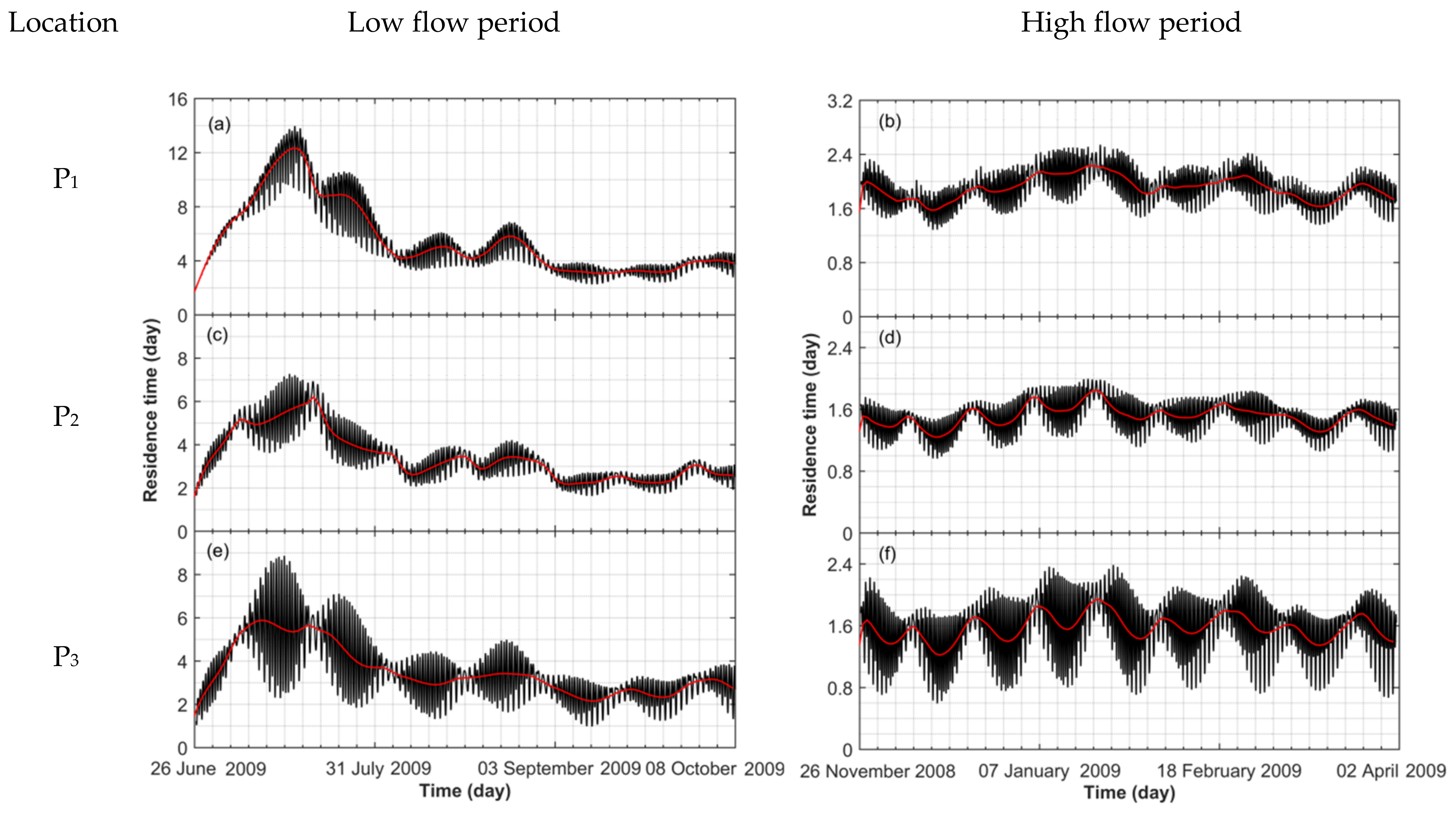
Figure 10.
Simulated values of the residence time at the: (a) P1; (b) P2; (c) P3 (see Figure 3) for the low period and simulated values of the residence time at the: (d) P1; (e) P2, (f) P3 for the high flow period. In each panel, the back line indicates the instantaneous value, while the red curve presents the averaged value over 24 h taken to filter out tidal oscillation.

Figure 11.
Distribution of the residence time in the whole delta for the: (a) low; (b) high flow period. The color bar is cropped at 13 days in order to focus on the variation of the residence time in deltaic channels, and the unit is day.
Figure 11.
Distribution of the residence time in the whole delta for the: (a) low; (b) high flow period. The color bar is cropped at 13 days in order to focus on the variation of the residence time in deltaic channels, and the unit is day.

Figure 12.
Distribution of the exposure time in the whole delta for the: (a) low; (b) high flow period. The color bar is cropped at 13 days in order to focus on the variation of the exposure time in deltaic channels and the unit is day.
Figure 12.
Distribution of the exposure time in the whole delta for the: (a) low; (b) high flow period. The color bar is cropped at 13 days in order to focus on the variation of the exposure time in deltaic channels and the unit is day.

Figure 13.
Distribution of the return coefficient for the: (a) low; (b) high flow period.


Table 1.
Boundary and initial conditions for calculating the age in the domain of interest.
| Original Water | Renewing Water | |||||
|---|---|---|---|---|---|---|
| River Water | Total Renewing Water | |||||
| t = 0 | Co = 1 | αo = 0 | Cu = 0 | αu = 0 | Cr = 0 | αr = 0 |
| x ∈ Γu | Co = 0 | αo = 0 | Cu = 1 | αu = 0 | Cr = 1 | αr = 0 |
| x ∈ Γd | Co = 0 | αo = 0 | Cu = 0 | αu = 0 | Cr = 1 | αr = 0 |
© 2020 by the authors. Licensee MDPI, Basel, Switzerland. This article is an open access article distributed under the terms and conditions of the Creative Commons Attribution (CC BY) license (http://creativecommons.org/licenses/by/4.0/).
Share and Cite
MDPI and ACS Style
Pham Van, C.; De Brye, B.; De Brauwere, A.; Hoitink, A.J.F.; Soares-Frazao, S.; Deleersnijder, E. Numerical Simulation of Water Renewal Timescales in the Mahakam Delta, Indonesia. Water 2020, 12, 1017. https://doi.org/10.3390/w12041017
AMA Style
Pham Van C, De Brye B, De Brauwere A, Hoitink AJF, Soares-Frazao S, Deleersnijder E. Numerical Simulation of Water Renewal Timescales in the Mahakam Delta, Indonesia. Water. 2020; 12(4):1017. https://doi.org/10.3390/w12041017
Chicago/Turabian StylePham Van, Chien, Benjamin De Brye, Anouk De Brauwere, A.J.F. (Ton) Hoitink, Sandra Soares-Frazao, and Eric Deleersnijder. 2020. "Numerical Simulation of Water Renewal Timescales in the Mahakam Delta, Indonesia" Water 12, no. 4: 1017. https://doi.org/10.3390/w12041017
Note that from the first issue of 2016, this journal uses article numbers instead of page numbers. See further details here.