Cloud Computation Using High-Resolution Images for Improving the SDG Indicator on Open Spaces

Abstract

Open spaces are essential for promoting quality of life in cities. However, accelerated urban growth, in particular in cities of the global South, is reducing the often already limited amount of open spaces with access to citizens. The importance of open spaces is promoted by SDG indicator 11.7.1; however, data on this indicator are not readily available, neither globally nor at the metropolitan scale in support of local planning, health and environmental policies. Existing global datasets on built-up areas omit many open spaces due to the coarse spatial resolution of input imagery. Our study presents a novel cloud computation-based method to map open spaces by accessing the multi-temporal high-resolution imagery repository of Planet. We illustrate the benefits of our proposed method for mapping the dynamics and spatial patterns of open spaces for the city of Kampala, Uganda, achieving a classification accuracy of up to 88% for classes used by the Global Human Settlement Layer (GHSL). Results show that open spaces in the Kampala metropolitan area are continuously decreasing, resulting in a loss of open space per capita of approximately 125 m² within eight years.

1. Introduction

Driven by the acceleration of urbanization across the globe, urban areas are expanding outwards but also densifying within the existing built-up area, leading to large-scale land conversion from open spaces into built-up areas. Many studies [1,2,3] emphasized the importance of open and in particular green spaces for livable cities. However, many citizens across the globe do not have easy access to open and green spaces in close proximity to their residence. The absence of open and green spaces has various negative impacts, e.g., lack of environmental quality (e.g., increased urban temperature [4]), health issues (e.g., increased risk of obesity [5]), lack of social interaction with neighbors [6]; insufficient spaces for evacuation in case of disasters [7] and missing spaces for economic and livelihood opportunities (e.g., informal street economy [6]). However, the amount of available open and green spaces differs dramatically across cities and regions [8]. For example, the share of green space per capita, important to promote walkability and good access to recreational spaces, differs between Hamburg (Germany) with 2750 m² per capita and Tijuana (Mexico) with 2 m² per capita [9]. In general, the absence of green spaces accounts according to the World Health Organization (WHO) for 3.3% of global death [10].

Urban planners and policy makers commonly aim for compact urban development, e.g., to support efficient infrastructure provision, walkable, and multi-functional urban neighborhoods. In this context, the provision of open public (green) spaces accessible to all citizens is crucial, but often not sufficiently available to citizens, in particular in rapidly developing urban areas. Therefore, SDG indicator 11.7.1 “average share of the built-up area of cities that is open space for public use for all, by sex, age and persons with disabilities”, part of Goal 11 “Make cities and human settlements inclusive, safe, resilient and sustainable”, promotes the importance of public open spaces, both gray (open spaces without vegetation cover such as urban squares) and green spaces (open spaces with vegetation cover such as parks). The indicator (share of built-up area that is open: Built_Open) compares the total built-up area of an urban agglomeration with the area that is open space (gray and green spaces). To operationalize this indicator, the continuously built-up area of an urban agglomeration (thus not the administrative city) is mapped with publicly available satellite images (e.g., Landsat, Sentinel) and the amount of open spaces and the street area (which are also important spaces for interaction) are mapped. The indicator (Built_Open) is computed following [8]:

$$Buil{t}_{Open}=\frac{\mathrm{Total} \mathrm{area} \mathrm{open} \mathrm{public} \mathrm{space} + \mathrm{Total} \mathrm{area} \mathrm{of} \mathrm{streets}}{\mathrm{Total} \mathrm{built} \mathrm{up} \mathrm{area} \mathrm{the} \mathrm{urban} \mathrm{agglomeration}}$$

(1)

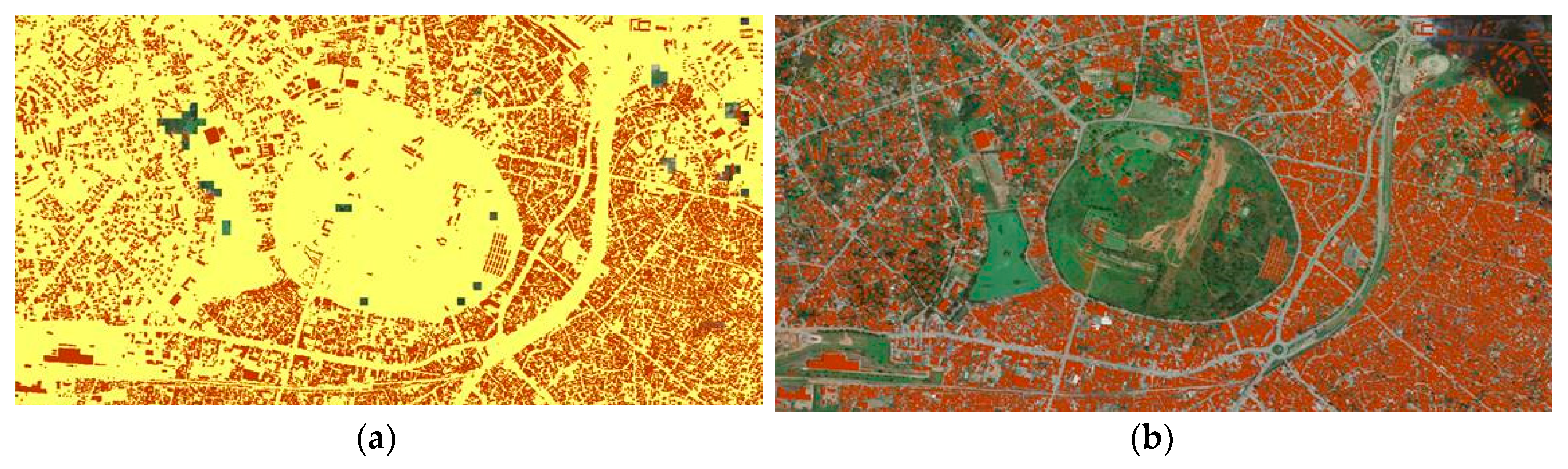
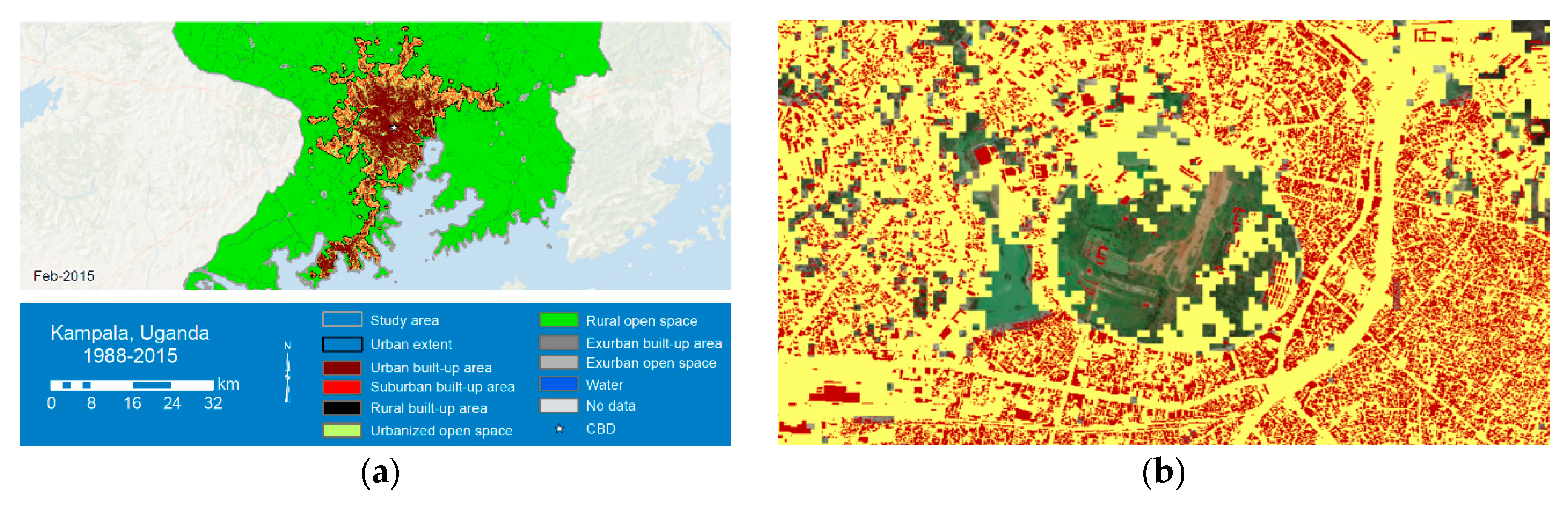
SDG indicator 11.7.1, presently not included in the SDG database (https://unstats.un.org/sdgs/indicators/database/) due to its operationalization complexity, has been piloted in over 250 cities [8] using moderate- to high-resolution satellite images. For example, the Global Urban Footprint (GUF) layer developed by the German Aerospace Center (DLR) [11,12] and the Global Human Settlement Layer (GHSL) developed by the European Commission Joint Research Centre (JRC) [13] use such images and provide a global and multi-temporal built-up area dataset as publicly available data repositories [13]. However, the mapped built-up areas of such products (e.g., the GHSL) are rather coarse due the resolution (approximately 30 m), which omits smaller open spaces and classifies them as built-up areas. Figure 1 shows the GHSL (built-up areas in yellow) for a part of the city of Kampala, where a large part of the non-built-up area is included as built-up area. The detailed built-up area structure is represented by the building footprints (in red). However, it should be noted that the large round-shaped green area is Kabaka’s Palace, the residence of the King of Buganda, and as such, it is a large green space (with important environmental functions) but not a public open space. Due to the absence of public open space inventories for most cities in the Global South, UN-Habitat [8] suggests the use of earth observation (EO) data “to identify potential open public spaces”, which include the streets and in particular green spaces within the city boundary, which play an important environmental role. Such an assessment is available, e.g., at the Urban Centre Database of JRC, which registers the share of the global population living in dense green areas. In 2014, this share was 23% for all urban centers across the globe, while this was 27% for the city of Kampala, thus larger as compared to the African average with only 20% [14]. In contrast, the Atlas of Urban Expansion [15] (also using Landsat images), produced in cooperation with UN-Habitat (http://www.atlasofurbanexpansion.org/), concludes that approximately 41% of the urbanized area in the agglomeration of Kampala was open space (in 2015). Here, open spaces are defined as “open countryside, forests, cultivated lands, parks, vacant lands that have not been subdivided, cleared land, and water bodies: seas, rivers, lakes, and canals” [15]. However, also for the Atlas of Urban Expansion, a similar problem as described above is shown, i.e., open spaces are mainly outside the city (Figure 2a), and small internal gray and green open spaces are partially omitted due to the coarse resolution of imagery used (Figure 2b).

Two main bottlenecks exist towards achieving a spatially more detailed representation of the urban built-up area structure—the access to high-resolution satellite images and the computational costs of processing data at the scale of urban agglomerations. Very-high-resolution (VHR) images (e.g., Pleiades) are available to commercial rates, with costs of typically more than 10 Euros per km². Taking the example of Kampala, and the urban area mapped by the GHSL (528 km²) or the Atlas of Urban Expansion (513 km²), this would arrive at an image data cost of more than 5000 Euros for one city. To upscale this to all cities (e.g., as included in the JRC database of urban centers), which is approximately 13,000 cities, and for different years, this would generate enormous image data costs (for all cities of the database this would be close to 10 million Euros for one year). Furthermore, the processing of VHR image data requires enormous computational resources. Both problems (image and computational costs) can be at least partially solved for research purposes by high-resolution image repositories, i.e., the Planet image data repository (https://www.planet.com/markets/education-and-research/), which enables access to high and very-high-resolution images (ranging from 1 to 5 m spatial resolution) and Google Earth Engine (GEE) [16], providing an efficient computational environment. The study addresses the above-identified bottlenecks (access to high-resolution satellite imagery and the computational costs) by proposing a framework that is built on cloud computation, open imagery and open reference data (for research), with minimal manual interaction and tuning to support future scalability. Therefore, the aim of this study is to analyze whether high-resolution (HR) images (in particular, RadipEye images) provide a better estimation of the presence of built-up and open spaces in support of SDG indicator 11.7.1 at the urban scale. The processing of the images and mapping of built-up areas is carried out within GEE, a very efficient cloud computation environment. The paper is divided into the following sections. Section 2 provides an overview of the study area, the city of Kampala, and describes the input data. Section 3 elaborates on the methodology to assess the current GHSL for the study area and the machine learning workflow used to map built-up and non-built-up areas. Section 4 provides the results and shows the potential to ease the calculation of SDG indicator 11.7.1. Section 5 discusses the role of EO to provide consistent data for SDG indicators and the new avenues opened by cloud computation, and Section 6 details the main conclusions.

2. Study Area and Input Data

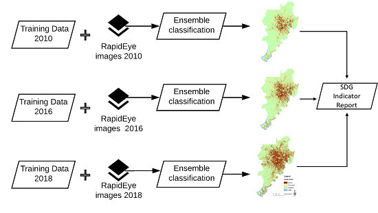
In this section, we present an overview of the study area, the specification of the HR images used, and the workflow of the ensemble algorithm applied to estimate a) Built_Open for 2010, 2016 and 2018, respectively, and b) changes in Built_Open.

2.1. Overview of the Study Area

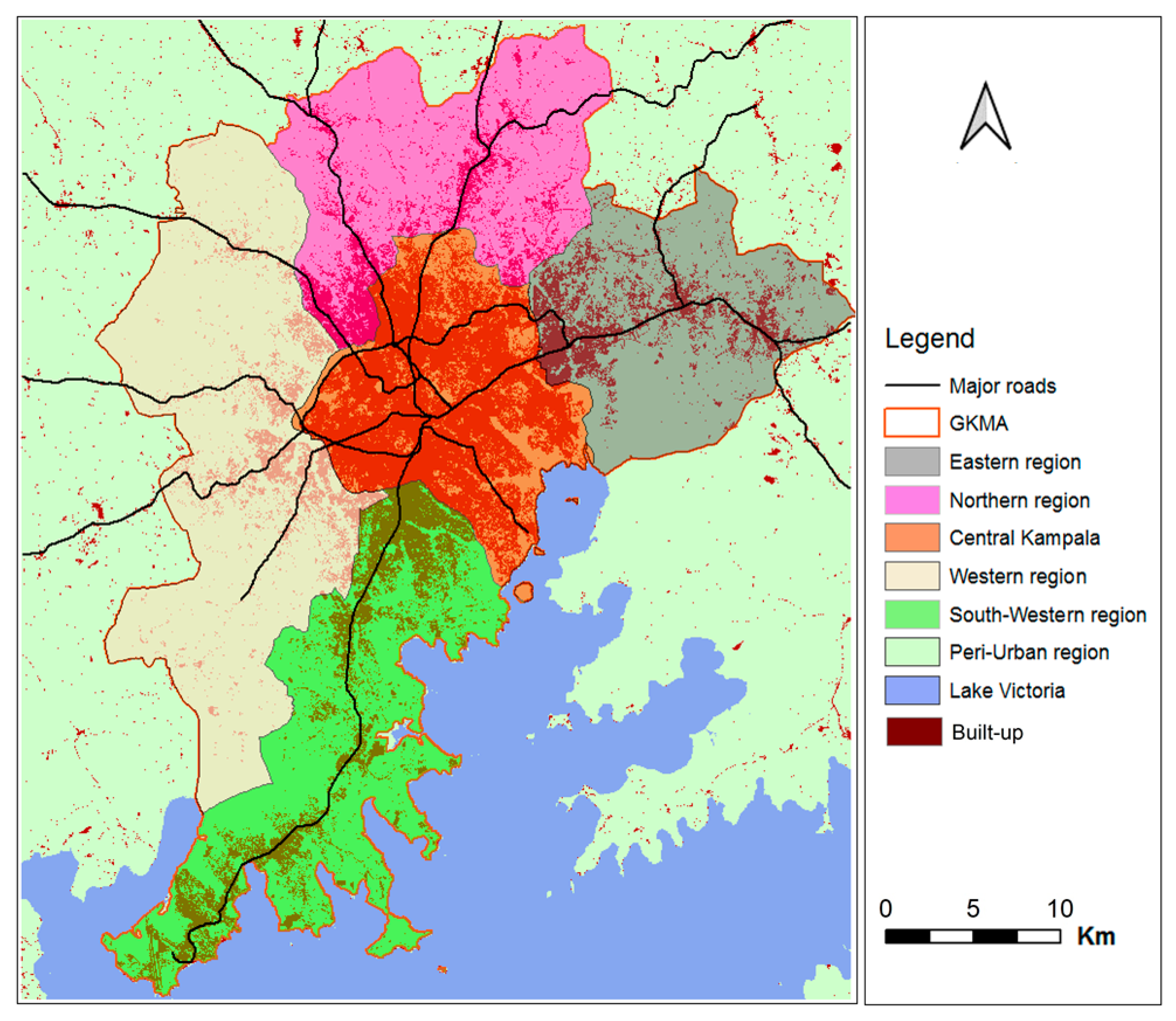
The urban agglomeration of Kampala is split into the city of Kampala (1.65 million estimated inhabitants in 2019) governed by the Kampala Capital City Authority (KCCA) and the Greater Kampala Metropolitan Area (GKMA) (Figure 3), with an estimated population of approximately 3.2 million [17]. Large parts of the urban agglomeration are informal, and inhabitants are deprived of basic service provision. Informal areas commonly have high built-up areas and population density and inhabitants do not have good access to gray and green open spaces. The urban agglomeration (estimated by the GHSL with a population of 3.5 million) has a very high annual population growth rate of 5.7% and belongs to the fastest growing African cities [18]. The central city is very densely built up, with the exception of wetlands and other protected areas [19].

2.2. Input Data

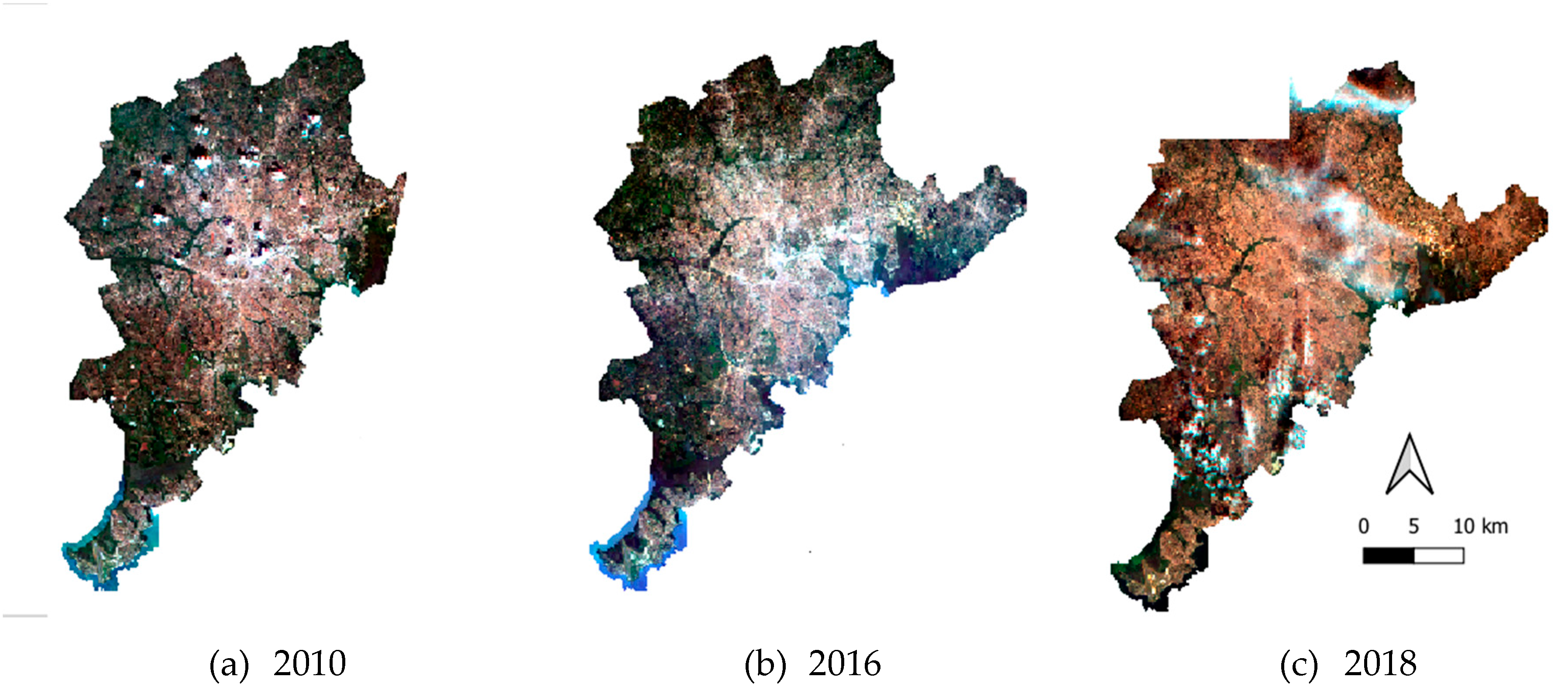
Three datasets of orthorectified RapidEye images (analytic ortho scene products) were compiled for the Kampala metropolitan area [20] for 2010, 2016 and 2018. Such images, obtained from the Planet platform [21], contain five bands (blue, green, red, red edge, near-infrared), and have a spatial resolution of 6.5 meters, resampled to 5 meters. Images were selected with less than 10% of cloud coverage [22] for the study area. Cloud coverage of images is a general problem in tropical regions, and often no annual cloud-free mosaic can be obtained. Figure 4 illustrates the image mosaic in natural color composition for years (a) 2010, (b) 2016, and (c) 2018.

The reference (training and validation) data was collected combining different sources (

Table 1. Overview of source for training data.

Year	Data Source	Criteria	Total Points
2010	Municipal Map City of Kampala	Built-up: Buildings with an area >100 m2 Centre line of roads: 4m buffer around roads Vegetation: natural vegetation areas Water: Water bodies	3996
2016	ESA Africa Land cover map of 2016	Built-up 2010 (check for changes): Buildings with an area >100 m2 Centre line of roads 2010 (check for changes): 4m buffer around roads ESA vegetation: grass, greenfield, forest, garden, brownfield, greenspace Water: Water bodies	3931
2018	OSM	Built-up: buildings with an area >100 m2 Centre line of roads: 4m buffer around roads Vegetation: grass, greenfield, forest, garden, brownfield, greenspace Water bodies	3893

) from which 1000 random points were selected for each class and for each year, followed by consistency checks that removed ambiguous samples (e.g., samples of roads that are located at edges of buildings). For 2010, we used municipal data for the city of Kampala, i.e., building footprints, roads and land use data. Building samples were randomly selected from the building data with a roof area of more than 100 m², which allowed excluding small isolated structures. For the gray open space class, samples were selected along major and secondary roads, ensuring that samples did not fall on roofs. Water and vegetation samples were selected in the zones of natural areas. For 2016, we extracted reference data from the ESA Africa land cover map (http://2016africalandcover20m.esrin.esa.int/). As the 2016 data were of the coarser resolution, the following rules were implemented. Samples of buildings and roads from 2010 were used and it was determined whether the areas changed between 2010 and 2016, as well as whether the ESA land cover map highlighted them as built-up areas. Water points from 2010 were also used and changes in the waterline (Lake Victoria) were updated. Vegetation points were extracted from the ESA Africa land cover map (restricting the selection to the classes trees, shrubs and grassland). For 2018, we used the OSM dataset [23] for the city of Kampala; we only extracted buildings with an area larger than 100 m². For gray open spaces, samples were selected along major and secondary roads, ensuring that samples did not fall on roofs. Water and vegetation samples were selected in the zones of natural areas.

3. Methodology

3.1. Assessment of the GHSL for the Study Area

The GHSL shows that the city of Kampala is almost completely built up. However, when comparing the GHSL with local reference data on building footprints, major differences are apparent (Figure 1b). To understand these differences, the building footprints of the city of Kampala from 2010 are compared with the GHSL layer of 2014 (closest to the building layer). Taking 20,000 random points, the agreement between building footprints and the GHSL built-up area is compared using the following thresholds for the municipal building footprint layer aggregated to the cell size of 38 m (cell size of the GHSL):

• Taking 50% built-up area (building footprints) as the threshold for classifying a cell as built-up area.
• Taking 10% built-up area (building footprints) as the threshold for classifying a cell as built-up area.
• Taking more than 0% built-up area (building footprints) as the threshold for classifying a cell as built-up area.

3.2. Calculation of the Built_Open Indicator

Methods to calculate SDG indicator 11.7.1 normally involve three steps. Step 1 is the delimitation of the built-up area of the city, step 2 is the estimation and validation of open public spaces and step 3 is the estimation of the total area allocated to the streets [8]. Step 1 includes the classification of Landsat images and spatial analysis to determine the urban-ness of pixels. The second step is the conventional approach for cities that lack an inventory of open public spaces and requires the use of remotely sensed imagery to identify and, subsequently, validate potential open public spaces, e.g., via costly and time-consuming field surveys [24]. The third step can be performed by computing the sum of the areas covered by each street where the width and length of are known, or by taking samples in the study area and digitizing the streets located in those samples to later compute a street area average that will be used to estimate the total area covered by streets.

In this study, we present an alternative approach for the computation of the Built_Open indicator based on cloud computation and machine learning classification of HR images. To do so, we used the city delimitation given by World Bank [20] as a boundary for the study area. The ground truth data required to train the machine learning algorithm was extracted from different sources, including municipal data and OSM data [23]. We also compare the Built_Open indicator for different years, namely 2010, 2016, and 2018.

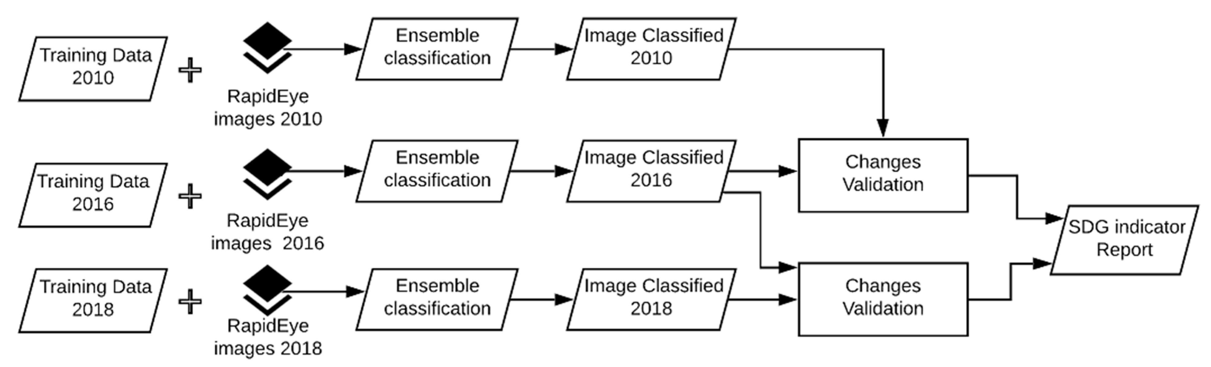
For the reference years, i.e., 2010, 2016, and 2018, we composed image mosaics that were classified using an ensemble classifier that is a machine learning algorithm that combines several base classifiers under certain rules. The base classifiers were trained and tested using training data extracted from different sources (see Section 2.1). For that purpose, each training dataset was randomly and proportionally split into three sets. Two sets were used to train and assess the performance, e.g., accuracy, of the base classifiers, and the remaining set was applied to evaluate the result of the ensemble classification (see Figure 5). To improve the consistency of changes, rules that follow the GHSL were also implemented [25]. For this purpose, a water mask was generated, which was applied for all years, and further checking backward and forward changes in vegetation and (built-up) areas. After this validation of changes, we calculated the Built_Open index following the formula presented in (1).

3.2.1. Ensemble Classification

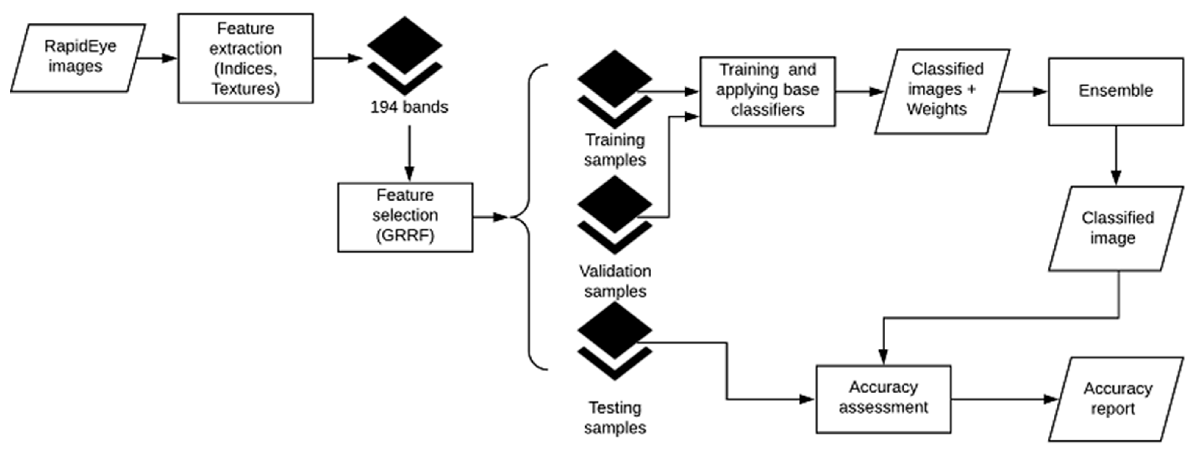
Figure 6 shows the workflow of the image classification applying an ensemble, including the pre-processing step to perform both feature extraction and feature selection and the training and application of base classifiers that formed the ensemble [26].

• Data pre-processing

Each image dataset was pre-processed to extract spectral and textural features (

Table 2. Features extracted from a single multi-spectral RapidEye image [GLCM: Gray Level Co-occurrence Matrix].

Features	Features per Image
Spectral image bands	5
Indices	9
GLCM-based textural features	180
Total	194

), i.e., indices [27,28,29,30,31,32,33] and Gray Level Co-occurrence Matrix (GLCM)-based textures of image bands [34,35]. Spectral features are known to be useful in the determination of green areas or water bodies, whereas textural features are regularly applied to identify built-up areas [36,37,38]. Textural features were extracted as the average of their values in four directions (0, 45, 90, 135) for two windows sizes: 3x3 and 5x5 pixels.

Table 3. Indices and formulas. Rapid-eye band name abbreviations are: R = red, RE = red edge, G = green, B = blue and NIR = near infrared.

Indices	Formula
Enhanced Vegetation Index (EVI)	2.5 × (NIR − R)/(NIR +6 × R − 7.5 × B + 1)
Transformed Chlorophyll Absorption in Reflectance Index (TCARI)	3 × ((RE − R) − 0.2 × (RE − G) × (RE/R))
Soil Adjusted Vegetation Index (SAVI)	(1 + L) × (NIR − R)/(NIR + R + L), where L = 0.5
Modified Soil Adjusted Vegetation Index (MSAVI)	$0.5\ast (2\ast NIR+1-\sqrt{{\left(2\times NIR+1\right)}^2-8\times \left(NIR-R\right)})$
Visible Atmospherically Resistance Index (VARI)	(G − R)/(G + R − B)
Green Leaf Index (GLI)	(2 × G − R − B)/(2 × G + R + B)
Normalized Difference Vegetation Index (NDVI)	(NIR − R)/(NIR + R)
Normalized Difference Water Index with green band (NDWIGreen)	(G − NIR)/(G + NIR)
Normalized Difference Water Index with red band (NDWIRed)	(R − NIR)/(R + NIR)

provides formulas and abbreviations for spectral indices;

Table A1. Textural feature formulas from Gray Level Co-occurrence Matrix, as described in [26,34].

Name/Formula	Name/Formula
Angular Second Moment $f_1={\displaystyle {\displaystyle \sum }_{i=1}^{N_g}}{\displaystyle {\displaystyle \sum }_{j=1}^{N_g}}{\left\{p\left(i,j\right)\right\}}^2$	Contrast $f_2={\displaystyle {\displaystyle \sum }_{n=0}^{N_{g-1}}}{n}^2\left\{{{\displaystyle {\displaystyle \sum }_{i=1}^{N_g}}{\displaystyle {\displaystyle \sum }_{j=1}^{N_g}}p\left(i,j\right)}_{\left|i-j\right|=n}\right\}$
Correlation $f_3={\displaystyle {\displaystyle \sum }_{i=1}^{N_g}}{\displaystyle {\displaystyle \sum }_{j=1}^{N_g}}\frac{\left(i,j\right)p\left(i,j\right)-{\mu }_x{\mu }_y}{{\sigma }_x{\sigma }_y}$	Variance $f_4={\displaystyle {\displaystyle \sum }_{i=1}^{N_g}}{\displaystyle {\displaystyle \sum }_{j=1}^{N_g}}{\left(i-\mu \right)}^{2}p\left(i,j\right)$
Inverse Difference Moment $f_5={\displaystyle {\displaystyle \sum }_{i=1}^{N_g}}{\displaystyle {\displaystyle \sum }_{j=1}^{N_g}}\frac{1}{1+{\left(i-j\right)}^2}p\left(i,j\right)$	Sum Average $f_6={\displaystyle {\displaystyle \sum }_{i=2}^{2N_g}}i{p}_{x+y}\left(i\right)$
Sum Variance $f_7={\displaystyle {\displaystyle \sum }_{i=2}^{2N_g}} {\left(i-f_8\right)}^2{P}_{x+y}\left(i\right)$	Sum Entropy $f_8=-{\displaystyle {\displaystyle \sum }_{i=2}^{2N_g}}{p}_{x+y}\left(i\right)log\left\{p_{x+y}\left(i\right)\right\}$
Entropy $f_8=-{\displaystyle {\displaystyle \sum }_{i=2}^{2N_g}}{p}_{x+y}\left(i\right)log\left\{p_{x+y}\left(i\right)\right\}$	Difference Variance $f_{10}=$ variance of $p_{x-y}$
Difference Entropy $f_{11}={\displaystyle {\displaystyle \sum }_{i=0}^{N_{g-1}}}{p}_{x-y}\left(i\right)log\left\{p_{x-y}\left(i\right)\right\}$	Information Measures of Correlation 1 $f_{12}=\frac{HXY-HXY1}{\max \left\{HX,HY\right\}}$where, $HXY=-{\displaystyle {\displaystyle \sum }_{i=1}^{N_g}}{\displaystyle {\displaystyle \sum }_{j=1}^{N_g}}p\left(i,j\right)\log \left(p\left(i,j\right)\right)$ $HXY1=-{\displaystyle {\displaystyle \sum }_{i=1}^{N_g}}{\displaystyle {\displaystyle \sum }_{j=1}^{N_g}}p\left(i,j\right)\log \left\{p_x\left(i\right)p_y\left(j\right)\right\}$ $HX$ and $HY$ are entropies of ${\mathrm{p}}_x$ and $p_y$
Information Measures of Correlation 2 $f_{13}={\left(1-e^{\left[-2.0\left(HXY2-HXY\right)\right]}\right)}^{1/2}$, where $HXY2=-{\displaystyle {\displaystyle \sum }_{i=1}^{N_g}}{\displaystyle {\displaystyle \sum }_{j=1}^{N_g}}{p}_x\left(i\right)p_y\left(j\right)\log \left\{p_x\left(i\right)p_y\left(j\right)\right\}$	Maximal Correlation Coefficient $f_{14}={\left(\sec \mathrm{ond} \mathrm{largest} \mathrm{eigen} \mathrm{value} \mathrm{of} \mathrm{Q}\right)}^{\frac{1}{2}}$ where $Q_{\left(i,j\right)}={\displaystyle {\displaystyle \sum }_{k=0}^{N_{g-1}}}\frac{p\left(i,k\right)p\left(j,k\right)}{p_x\left(i\right)p_y\left(k\right)}$
Dissimilarity $f_{15}={\displaystyle {\displaystyle \sum }_{i=1}^{N_g}}{\displaystyle {\displaystyle \sum }_{j=1}^{N_g}}{\left|i-j\right|}^{2}p\left(i,j\right)$

and

Table A2. Textural features included in the classification, as explained in [25,34].

Description	Formula
Inertia	$I\left(\delta ,T\right)={\displaystyle {\displaystyle \sum }_{i=0}^{L-1}}{\displaystyle {\displaystyle \sum }_{j=0}^{L-1}}{\left(i-j\right)}^{2}s\left(i,j,\delta ,T\right)$.
Cluster shade	$A\left(\delta ,T\right)={\displaystyle {\displaystyle \sum }_{i=0}^{L-1}}{\displaystyle {\displaystyle \sum }_{j=0}^{L-1}}{\left(i+j-{\mu }_i-{\mu }_j\right)}^{3}s\left(i,j,\delta ,T\right)$
Cluster prominence	$B\left(\delta ,T\right)={\displaystyle {\displaystyle \sum }_{i=0}^{L-1}}{\displaystyle {\displaystyle \sum }_{j=0}^{L-1}}{\left(i+j-{\mu }_i-{\mu }_j\right)}^{4}s\left(i,j,\delta ,T\right)$

, in Appendix A, list formulas for textural features.

It was necessary to reduce the number of features used to train and apply the classifiers to ensure timely execution of those classifiers in GEE. To conduct feature reduction, we applied a Guided Regularized Random Forest (GRRF [39]) that is a feature selection algorithm based in Random Forest [40]. Then, we applied a Support Vector Machine [41] classifier with a Gaussian kernel to the top ten most accurate subsets of features returned by GRRF. The subset of features with the highest accuracy in both (GRRF and SVM) was selected. This process was performed for each dataset separately. This approach selected the most informative feature for our classification task among similar features, e.g., NDVI and EVI. GRRF does not require a prior parameter setup and ensures the selection of non-redundant and informative features improving the classification accuracy when applying a Random Forest algorithm afterwards, although a small negative impact on accuracy has been reported for regression tasks [39]. On the other hand, SVM is a robust and widely applied machine learning algorithm that generalizes well when the number of input features is large, and the training data are limited [41,42]. A shortcoming of SVM is the parameter setting that is commonly tackled, also in this study, by grid search using cross-validation [43].

• Ensemble classifier

The ensemble classifier combined nine base classifiers, meaning three classifier instances of Random Forest, SVM with a Gaussian kernel and SVM with a polynomial kernel, respectively. Those classifiers were selected as they provide state-of-the-art performance [44]. Base classifiers were trained and applied separately using a modified leave-one-out method in which the training set is stratified and randomly partitioned into k (5) equally sized subsamples. Each base classifier was trained with k − 1 subsamples, leaving one subsample out [26]. Using different seeds to generate the subsamples, these methods allowed us to generate at least nine subsets, ensuring an odd number of base classifiers in the ensemble. The individual influence of each base classifier was weighted by its performance in a validation dataset, i.e., the Overall Accuracy (OA) of each base classifier is used as a weight in the ensemble [26]. The OA of the ensemble classification is reported for each year.

3.2.2. Consistency of Changes

A water mask, similar to the workflow proposed by the GHSL [25], was calculated to improve the consistency of changes and reduce noise. This mask was applied to each classified image and pixels that were initially classified as water but did not belong to the water mask were reclassified as follows:

• The classified mosaic of 2016 was taken as a reference because this dataset obtained a higher accuracy in the classification.
• Pixel values in the 2016 mosaic were replaced by the pixel value in the 2010 mosaic if those belong to built-up areas or gray spaces.
• Pixel values in 2010 were replaced by gray spaces as visual inspection confirmed that these pixels were wrongly classified as water, mainly being areas of shadows (e.g., along roads).
• Pixel values in the 2018 mosaic were substituted by the pixel value of the classified mosaic in the previous reference year, i.e., the classified mosaic for 2016.

Concerning changes in built-up areas, and taking the 2016 mosaic as a reference, we assumed that built-up areas in 2016 were also built-up areas in 2018, roads in 2016 were also roads in 2018 and that vegetation areas in 2016 were vegetation areas in 2010. Pixels were reclassified accordingly. To consistently calculate a Built_Open index, we created a common mask to achieve the same area coverage because it was not possible to find less than 10% cloud coverage scenes for the entire study area. These consistency rules also enabled the use of areas of cloud coverage without masking. This workflow allowed for minimal manual interaction, which is important for the development of scalable methods.

4. Results

4.1. The Strength and Weaknesses of the GHSL for Built-Up and Open Space Mapping

A comparison of the GHSL with the building footprints is presented in

Table 4. Comparing the built-up area classification of the GHSL with building footprints: (1) without aggregation and (2–4) with aggregation to the 38 m cell size.

	(1) Building Level	(2) 50% Built up	(3) 10% Built up	(4) >0% Built up
Overall Accuracy	0.354	0.268	0.711	0.836
Kappa	0.075	0.022	0.395	0.564

. The results show that when using the 10% threshold (i.e., 10% of a 38 by 38 m cell is covered by buildings), the accuracy of the GHSL is 71%, whereas the accuracy is 84% when there are any built-up areas. However, when comparing the sample point locations (building footprints and the GHSL), the GHSL shows an accuracy of 35%. Hence, the GHSL classifies large areas that are non-built-up areas as built-up areas (see example in Figure 1). Thus, the GHSL depicts the presence of any area of buildings within the 38 m cell very well; however, this limits the capability to show non-built-up (green or gray) spaces, particularly small spaces. Such spaces are being aggregated and are often omitted, which is a problem when using this data in the calculation of Built_Open for SDG indicator 11.7.1.

4.2. Image Classification and Built_Open Indicator

The feature selection approach adopted (see Section 2.2) produced the list of features presented in

Table 5. Selected features per year [b1: band 1, b2: band 2, b3: band 3, b4: band 4, b5: band 5, asm: angular second moment, contrast: contrast, corr: correlation, var: variance, idm: inverse difference moment, savg: sum average, svar: sum variance, sent: sum entropy, ent: entropy, dvar: difference variance, dent: difference entropy, imcorr1: information measures of correlation 1, diss: dissimilarity, inertia: inertia, shade: cluster shade, and prom: cluster prominence].

Feature\Year	2010	2016	2018
Image bands	b2, b5	b1, b3, b4, b5	b1, b5
Indices	NDWIRed, VARI	NDWIGreen, TCARI, VARI	GLI, NDWIRed, TCARI, VARI
Textural—3 × 3		b3_inertia, b3_shade, b5_dvar, b5_imcorr1	b1_sent, b2_prom, b3_savg, b4_savg, b5_var
Textural—5 × 5	b2_dvar, b3_inertia, b3_savg, b3_var, b4_contrast, b4_dvar, b4_var b5_contrast, b5_savg, b5_dvar, b5_corr	b3_dvar, b3_savg, b1_savg, b2_idm, b4_dent, b4_dvar, b5_asm, b5_contrast, b5_corr, b5_dent, b5_dvar, b5_ent, b5_idm, b5_imcorr1, b5_prom, b5_savg, b5_sent, b5_svar	b1_asm, b1_shade, b2_dvar, b2_savg, b2_shade, b3_savg, b3_shade, b4_inertia, b4_shade, b5_asm, b5_corr, b5_dent, b5_diss, b5_idm, b5_imcorr1, b5_prom, b5_savg, b5_sent, b5_svar
Total	15	29	30

, where textural features, in particular, those calculated using a window of size 5 × 5, are predominant. Meaning that these textural features are more informative when determining our classes. The index Visible Atmospherically Resistance Index (VARI) was selected in the three datasets, whereas Transformed Chlorophyll Absorption in Reflectance Index (TCARI) was selected for years 2016 and 2018. Such indices are well known for their utility in the identification of vegetation cover. The Normalized Difference Water Index with red band (NDWI_Red) also contributes to the identification of classes as it was selected in two datasets, 2010 and 2018.

Table 6. Assessment of Overall Accuracy (OA) using four classes (built-up area, gray spaces, green spaces and water) and three classes (GHSL classes: built-up area, non-built-up area and water).

Year	2010	2016	2018
OA 4 classes	0.78	0.83	0.73
OA 3 classes	0.84	0.88	0.86

presents the OA for each year. When the mosaics are reclassified to only three classes (GHSL classes, i.e., built-up area, non-built-up area and water surface), the OA increased considerably. This is because the class non-built-up area is aggregated, which contributes to improving the accuracy of the produced classification. The highest accuracy was achieved for the mosaic of 2016; this image was also 100% cloud free. The lowest accuracy is reported for the mosaic of 2018.

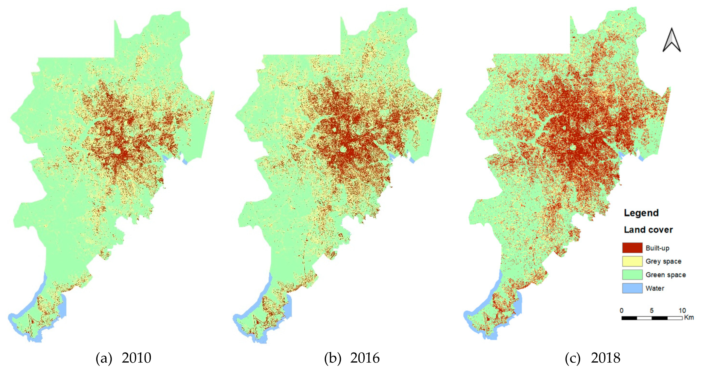
Figure 7 presents the classified mosaics for (a) 2010, (b) 2016, and (c) 2018. It shows the dynamic of the city, e.g., the vegetation cover decreases, whereas built-up areas gain more spaces. This increase in dense built-up areas occurs mainly in the core of the city because buildings are not distributed along the whole area of the city. These changes are quantified and presented in

Table 7. Land cover statistics per year in hectares (ha), the indicator Built_Open per year in ha, and the Built_Open per capita/year in m².

Year	2010	2016	2018
Built-up area	9087.40	14,698.49	24,374.61
Green space	63,608.26	54,998.31	48,984.30
Gray space	18,263.67	21,230.23	17,600.43
BuiltOpen	9.00	5.19	2.73
BuiltOpen per capita in m2	294.97	212.80	170.15

. The index Built_Open is reported there as well. These results show that the amount of open space continuously declines and when calculating the amount of open space per capita (using the WorldPop population data [45] of the respective years), the share reduces from approximately 300 to 170 m² between 2010 and 2018.

Figure 8 illustrates the dynamic of built-up area in the city. There is a sustained increase in the built-up area, but it becomes evident that the intensity of the urbanization boosted between 2016 and 2018.

5. Discussion

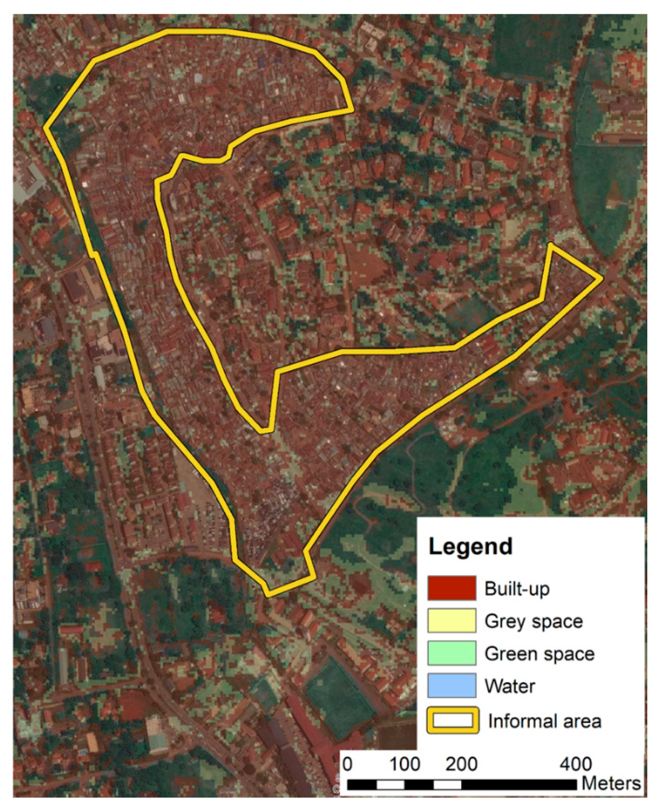
This study proposes an alternative method to calculate the Built_Open index based on HR images and machine learning classification methods. The proposed method uses free-for-research available HR images and a free-for-research cloud platform such as GEE. Building on computational efficiency, HR images and harvesting of reference data from available databases open opportunities to scale up the method beyond this pilot case study. Based on the case study, we could demonstrate that the combination of data within GEE made it feasible to monitor the temporal dynamics of the Built_Open index at a relatively high temporal granularity. At the metropolitan scale, such data enable monitoring the progress towards achieving SDG 11.7.1, in particular when adding local information about public access and population data split into gender, age groups and disabilities. Using a publicly accessibly population dataset (WorldPop [45]), our results showed that the share of open space per capita almost halved between 2010 and 2018, with a loss of 125 m² per capita (Table 7). Having such spatially detailed data allows specifying the shares of gray and green open spaces in different parts of the metropolitan area. For example, Kampala city is very densely built up with limited access to gray and green open spaces in the immediate surroundings per person. Furthermore, there is a major difference in open space availability between planned and well-serviced areas as compared to informal and deprived areas. We used the available municipal data for 2010 to analyze this difference. Results show that all informal areas within the city had on average of 20% less open space as compared to planned areas (example area is shown in Figure 9).

The indicator presently calculated for this SDG, i.e., the Built_Open indicator, is a ratio between the open spaces and street space divided by the amount of built-up area [8]. As such, the indicator is difficult to interpret for policy making and the general public. The indicator Built_Open per capita in m², which would already include the aspect of the population into the equation, would be much easier to communicate to the general public. This indicator can be more easily quantified for cities across the globe, combining existing population data (e.g., WorldPop data [46]) and data on gray and green open spaces extracted by the proposed method in this paper.

The proposed method, when compared with the Landsat-based GHSL layer, captures the locations and patterns of open spaces much better. For comparison, we reduced our classification from four classes, which included two open space classes (gray and green), to one open space class (non-built-up area), available in the GHSL [13,25], and results showed an overall good performance of our method. However, for the proposed method, the availability of training data is also a limitation. In this context, crowdsourced data such as OSM proved to be beneficial, although the quality differs across regions [47,48]. Further, citizens’ right of access is not captured by the mapping output. However, it is necessary to effectively determine the accessibility to spaces that are classified as gray and green open spaces but could be restricted in their use/access for certain citizens. Further, OSM data does not provide a straightforward way to unpack city dynamics, as the temporal dimension that can be derived by the changeset element is not freely available due to privacy regulations in the European Union. Although it is possible to integrate deep neural network algorithms in GEE [16], these kinds of algorithms require larger training datasets that were not available for our study area. This is a regular situation in many cities in the global South, where the GHSL accuracy is also often relatively low as compared to Europe. We demonstrate here that state-of-the-art algorithms such as RF, SVM and their combination, i.e., an ensemble, obtained good performance for the purpose at hand and for a wide geographic area.

In general, the employed HR images have a strong advantage as compared to Landsat, due to the higher resolution of RapidEye. However, a limitation of the RapidEye images, in regard to land cover classification concerns, is the missing availability of a shortwave infrared (SWIR) band. A SWIR band is used in the calculation of several indices such as the Normalized Difference Build-up Index (NDBI) to improve land cover classification [49]. However, this limitation did not prevent achieving good accuracy during the image classification procedure. Studies (e.g., [50]) in the global North, using VHR commercial images, show that even higher classification accuracies can be achieved, but then sufficient and high-quality training data and commercial, high-cost images might not be easily accessible in the global South and might prevent covering large areas. For such situations, we highlight the potential of combining open data such as OSM datasets and free-for-research images and cloud computing platforms to scale up our methods and produce a global coverage of the Built_Open indicator also expressed in a meaningful sense for laypersons, i.e., Built_Open per capita.

6. Conclusions

This study presented a method to calculate the Built_Open index using a machine learning algorithm applied to HR images in a cloud computing environment. We demonstrated that the proposed method has the potential to support the monitoring of urban dynamics and to inform policy making in addressing the SDG 11 targets, currently limited by coarse resolution data that do not sufficiently allow quantifying open spaces. Thus, using EO-based information to calculate Built_Open per capita would allow supporting strategic urban planning aimed at urban sustainability, by providing an easily quantifiable indicator that shows one aspect of sustainability. We discussed the limitations of this study concerning the availability of ground truth data required to train machine learning models and showed that open data and volunteered geographic information (VGI) data support training and validation of such models. The developed method allows mapping the dynamics of open spaces, both gray and green spaces, and provides relevant base data for urban planning and management of cities, addressing a crucial aspect of the environmental quality of livability in cities. Future work includes extending our study to cover other cities where the GHSL presents problems in capturing the difference between built-up and open spaces, such as cities located in very arid regions.

References

- Douglas, O.; Lennon, M.; Scott, M. Green space benefits for health and well-being: A life-course approach for urban planning, design and management. Cities 2017, 66, 53–62. [Google Scholar] [CrossRef] [Green Version]
- UN-Habitat. Streets as Public Spaces and Drivers of Urban Prosperity; UN-Habitat: Nairobi, Kenya, 2013. [Google Scholar]
- Wicht, M.; Kuffer, M. The continuous built-up area extracted from ISS night-time lights to compare the amount of urban green areas across European cities. Eur. J. Remote Sens. 2019, 52, 58–73. [Google Scholar] [CrossRef]
- Wang, J.; Kuffer, M.; Sliuzas, R.; Kohli, D. The exposure of slums to high temperature: Morphology-based local scale thermal patterns. Sci. Total Environ. 2019, 650, 1805–1817. [Google Scholar] [CrossRef] [PubMed]
- Kim, J.-H.; Lee, C.; Sohn, W. Urban Natural Environments, Obesity, and Health-Related Quality of Life among Hispanic Children Living in Inner-City Neighborhoods. Int. J. Environ. Res. Public Health 2016, 13, 121. [Google Scholar] [CrossRef]
- Dayo-Babatunde, B.; Martinez, J.; Kuffer, M.; Kyessi, A.G. The Street as a Binding Factor: Measuring the Quality of Streets as Public Space within a Fragmenting City: The Case of Msasani Bonde la Mpunga, Dar es Salaam, Tanzania. In GIS in Sustainable Urban Planning and Management; van Maarsevee, M.F.A.M., Martinez, M., Flacke, J., Eds.; CRC Press: Boca Raton, FL, USA, 2018; pp. 183–201. [Google Scholar]
- Shrestha, S.R.; Sliuzas, R.; Kuffer, M. Open spaces and risk perception in post-earthquake Kathmandu city. Appl. Geogr. 2018, 93, 81–91. [Google Scholar] [CrossRef]
- UN-Habitat. Metadata Indicator 11.7.1: Average Share of the Built-up Area of Cities that is Open Space for Public Use for All, by Sex, Age and Persons with Disabilities; United Nations Statistics Division, Development Data and Outreach Branch: New York, NY, USA, 2018. [Google Scholar]
- OECD. Green Area per Capita; UN-Habitat: Nairobi, Kenya, 2018. [Google Scholar]
- WHO. Urban Green Spaces. Available online: https://www.who.int/sustainable-development/cities/health-risks/urban-green-space/en/ (accessed on 1 March 2020).
- Esch, T.; Thiel, M.; Schenk, A.; Roth, A.; Müller, A.; Dech, S. Delineation of urban footprints from TerraSAR-X data by analyzing speckle characteristics and intensity information. IEEE Trans. Geosci. Remote Sens. 2010, 48, 905–916. [Google Scholar] [CrossRef]
- Taubenböck, H.; Esch, T.; Felbier, A.; Wiesner, M.; Roth, A.; Dech, S. Monitoring urbanization in mega cities from space. Remote Sens. Environ. 2012, 117, 162–176. [Google Scholar] [CrossRef]
- Pesaresi, M.; Guo, H.D.; Blaes, X.; Ehrlich, D.; Ferri, S.; Gueguen, L.; Halkia, M.; Kauffmann, M.; Kemper, T.; Lu, L.L.; et al. A global human settlement layer from optical HR/VHR RS data: Concept and first results. IEEE J. Sel. Top. Appl. Earth Obs. Remote Sens. 2013, 6, 2102–2131. [Google Scholar] [CrossRef]
- Florczyk, A.J.; Melchiorri, M.; Corbane, C.; Schiavina, M.; Maffenini, M.; Pesaresi, M.; Politis, P.; Sabo, S.; Freire, S.; Ehrlich, D.; et al. Description of the GHS Urban Centre Database 2015; Public Release 2019; Version 1.0; Office of the European Union: Luxembourg, 2019. [Google Scholar]
- Angel, S.; Blei, A.M.; Parent, J.; Lamson-Hall, P.; Galarza-Sanchez, N.; Civco, D.L.; Thom, K. Atlas of Urban Expansion—2016 Edition; The NYU Urbanization Project: New York, NY, USA, 2016. [Google Scholar]
- Gorelick, N.; Hancher, M.; Dixon, M.; Ilyushchenko, S.; Thau, D.; Moore, R. Google Earth Engine: Planetary-scale geospatial analysis for everyone. Remote Sens. Environ. 2017, 202, 18–27. [Google Scholar] [CrossRef]
- Uganda Bureau of Statistics. Statistical Abstract; Uganda Bureau of Statistics: Kampala, Uganda, 2019. [Google Scholar]
- UN-Habitat. The State of African cities 2014. Re-imagining Sustainable Urban Transitions; UN-Habitat: Nairobi, Kenya, 2014. [Google Scholar]
- Pérez-Molina, E.; Sliuzas, R.; Flacke, J.; Jetten, V. Developing a cellular automata model of urban growth to inform spatial policy for flood mitigation: A case study in Kampala, Uganda. Comput. Environ. Urban Syst. 2017, 65, 53–65. [Google Scholar] [CrossRef]
- World Bank. Kampala Metropolitan Area Spatial Extent; World Bank: Washington, DC, USA, 2017. [Google Scholar]
- Planet Team. Planet Application Program Interface: In Space for Life on Earth. Available online: https://api.planet.com (accessed on 1 January 2019).
- Planet Team. Rapideye™ Imagery Product Specifications; Planet Labs Inc.: San Francisco, CA, USA, 2016. [Google Scholar]
- OpenStreetMap contributions. Planet Dump. 2017. Available online: https://planet.osm.org (accessed on 9 December 2018).
- Duque, J.C.; Patino, J.E.; Betancourt, A. Exploring the Potential of Machine Learning for Automatic Slum Identification from VHR Imagery. Remote Sens. 2017, 9, 895. [Google Scholar] [CrossRef] [Green Version]
- Pesaresi, M.; Ehrlich, D.; Ferri, S.; Florczyk, A.J.; Freire, S.; Halkia, M.; Julea, A.; Kemper, T.; Soille, P.; Syrris, V. Operating Procedure for the Production of the Global Human Settlement Layer from Landsat Data of the Epochs 1975, 1990, 2000, and 2014; Publications Office of the European Union: Luxembourg, 2016. [Google Scholar]
- Aguilar, R.; Zurita-Milla, R.; Izquierdo-Verdiguier, E.; de By, R. A Cloud-Based Multi-Temporal Ensemble Classifier to Map Smallholder Farming Systems. Remote Sens. 2018, 10, 729. [Google Scholar] [CrossRef] [Green Version]
- Louhaichi, M.; Borman, M.M.; Johnson, D.E. Spatially Located Platform and Aerial Photography for Documentation of Grazing Impacts on Wheat. Geocarto Int. 2001, 16, 65–70. [Google Scholar] [CrossRef]
- Huete, A.; Didan, K.; Miura, T.; Rodriguez, E.P.; Gao, X.; Ferreira, L.G. Overview of the radiometric and biophysical performance of the MODIS vegetation indices. Remote Sens. Environ. 2002, 83, 195–213. [Google Scholar] [CrossRef]
- Huete, A.R. A soil-adjusted vegetation index (SAVI). Remote Sens. Environ. 1988, 25, 295–309. [Google Scholar] [CrossRef]
- Haboudane, D.; Miller, J.R.; Tremblay, N.; Zarco-Tejada, P.J.; Dextraze, L. Integrated narrow-band vegetation indices for prediction of crop chlorophyll content for application to precision agriculture. Remote Sens. Environ. 2002, 81, 416–426. [Google Scholar] [CrossRef]
- Gitelson, A.A.; Kaufman, Y.J.; Stark, R.; Rundquist, D. Novel algorithms for remote estimation of vegetation fraction. Remote Sens. Environ. 2002, 80, 76–87. [Google Scholar] [CrossRef] [Green Version]
- McFeeters, S.K. The use of the Normalized Difference Water Index (NDWI) in the delineation of open water features. Int. J. Remote Sens. 1996, 17, 1425–1432. [Google Scholar] [CrossRef]
- Space4water. Normalized Difference Water Index (NDWI). Available online: http://space4water.org/taxonomy/term/1315 (accessed on 3 April 2020).
- Haralick, R.M.; Shanmugam, K.; Dinstein, I. Texture features for image classification. IEEE Trans. Syst. Man. Cybern. 1973, 3, 610–621. [Google Scholar] [CrossRef] [Green Version]
- Conners, R.W.; Trivedi, M.M.; Harlow, C.A. Segmentation of a high-resolution urban scene using texture operators. Comput. Vis. Graph. Image Process. 1984, 25, 273–310. [Google Scholar] [CrossRef]
- Shen, H.; Abuduwaili, J.; Ma, L.; Samat, A. Remote sensing-based land surface change identification and prediction in the Aral Sea bed, Central Asia. Int. J. Environ. Sci. Technol. 2019, 16, 2031–2046. [Google Scholar] [CrossRef]
- Wurm, M.; Weigand, M.; Schmitt, A.; Geiß, C.; Taubenböck, H. Exploitation of textural and morphological image features in Sentinel-2A data for slum mapping. In Proceedings of the Joint Urban Remote Sensing Event (JURSE), Dubai, United Arab Emirates, 6–8 March 2017; pp. 1–4. [Google Scholar]
- Pesaresi, M.; Gerhardinger, A.; Kayitakire, F. A robust built-up area presence index by anisotropic rotation-invariant textural measure. IEEE J. Sel. Top. Appl. Earth Obs. Remote Sens. 2008, 1, 180–192. [Google Scholar] [CrossRef]
- Izquierdo-Verdiguier, E.; Zurita-Milla, R. An evaluation of Guided Regularized Random Forest for classification and regression tasks in remote sensing. Int. J. Appl. Earth Obs. Geoinf. 2020, 88, 102051. [Google Scholar] [CrossRef]
- Rodriguez-Galiano, V.F.; Ghimire, B.; Rogan, J.; Chica-Olmo, M.; Rigol-Sanchez, J.P. An assessment of the effectiveness of a random forest classifier for land-cover classification. ISPRS J. Photogramm. Remote Sens. 2012, 67, 93–104. [Google Scholar] [CrossRef]
- Mountrakis, G.; Im, J.; Ogole, C. Support vector machines in remote sensing: A review. ISPRS J. Photogramm. Remote Sens. 2011, 66, 247–259. [Google Scholar] [CrossRef]
- Camps-Valls, G.; Gomez-Chova, L.; Calpe-Maravilla, J.; Martin-Guerrero, J.D.; Soria-Olivas, E.; Alonso-Chorda, L.; Moreno, J. Robust support vector method for hyperspectral data classification and knowledge discovery. IEEE Trans. Geosci. Remote Sens. 2004, 42, 1530–1542. [Google Scholar] [CrossRef]
- Kavzoglu, T.; Colkesen, I. A kernel functions analysis for support vector machines for land cover classification. Int. J. Appl. Earth Obs. Geoinf. 2009, 11, 352–359. [Google Scholar] [CrossRef]
- Leonita, G.; Kuffer, M.; Sliuzas, R.; Persello, C. Machine Learning-Based Slum Mapping in Support of Slum Upgrading Programs: The Case of Bandung City, Indonesia. Remote Sens. 2018, 10, 1522. [Google Scholar] [CrossRef] [Green Version]
- Linard, C.; Gilbert, M.; Snow, R.W.; Noor, A.M.; Tatem, A.J. Population Distribution, Settlement Patterns and Accessibility across Africa in 2010. PLoS ONE 2012, 7, 8. [Google Scholar] [CrossRef] [Green Version]
- Wardrop, N.A.; Jochem, W.C.; Bird, T.J.; Chamberlain, H.R.; Clarke, D.; Kerr, D.; Bengtsson, L.; Juran, S.; Seaman, V.; Tatem, A.J. Spatially disaggregated population estimates in the absence of national population and housing census data. Proc. Natl. Acad. Sci. USA 2018, 115, 3529. [Google Scholar] [CrossRef] [Green Version]
- Grippa, T.; Georganos, S.; Zarougui, S.; Bognounou, P.; Diboulo, E.; Forget, Y.; Lennert, M.; Vanhuysse, S.; Mboga, N.; Wolff, E. Mapping Urban Land Use at Street Block Level Using OpenStreetMap, Remote Sensing Data, and Spatial Metrics. ISPRS Int. J. Geo-Inf. 2018, 7, 246. [Google Scholar] [CrossRef] [Green Version]
- Mahabir, R.; Stefanidis, A.; Croitoru, A.; Crooks, A.; Agouris, P. Authoritative and volunteered geographical information in a developing country: A comparative case study of road datasets in Nairobi, Kenya. ISPRS Int. J. Geo-Inf. 2017, 6, 24. [Google Scholar] [CrossRef]
- Huang, C.; Yang, J.; Lu, H.; Huang, H.; Yu, L. Green Spaces as an Indicator of Urban Health: Evaluating Its Changes in 28 Mega-Cities. Remote Sens. 2017, 9, 1266. [Google Scholar] [CrossRef] [Green Version]
- Giezen, M.; Balikci, S.; Arundel, R. Using Remote Sensing to Analyse Net Land-Use Change from Conflicting Sustainability Policies: The Case of Amsterdam. ISPRS Int. J. Geo-Inf. 2018, 7, 381. [Google Scholar] [CrossRef] [Green Version]
Figure 1.
(a) The 2014 Global Human Settlement Layer (GHSL) (built-up areas in yellow) and building footprints (in red); (b) building footprints (in red) on top of a Google Earth image.
Figure 2.
(a) Atlas of Urban Expansion (2015); (b) building footprints (in red) on top of the built-up areas of the Atlas of Urban Expansion (gaps Google Earth image).
Figure 3.
Greater Kampala Metropolitan area and its administrative subdivisions (the background GHSL and main streets from OpenStreetMap (OSM).
Figure 4.
(a) Mosaic of RapidEyes scenes in the study area for 2010, (b) Mosaic of RapidEyes scenes in the study area for 2016, and (c) Mosaic of RapidEyes scenes in the study area for 2018.
Figure 5.
Overview of the methodology.
Figure 6.
Ensemble classifier—overview of the workflow.
Figure 7.
Classified mosaics for (a) 2010, (b) 2016, and (c) 2018.
Figure 8.
Built-up area dynamic between 2010 and 2018.
Figure 9.
An informal area surrounded by planned areas, with a much large BuiltOpen.