An Evaluation of Autonomous In Situ Temperature Loggers in a Coastal Region of the Eastern Mediterranean Sea for Use in the Validation of Near-Shore Satellite Sea Surface Temperature Measurements

Abstract

The coastal ocean is one of the most important environments on our planet, home to some of the most bio-diverse and productive ecosystems and providing key input to the livelihood of the majority of human society. It is also a highly dynamic and sensitive environment, particularly susceptible to damage from anthropogenic influences such as pollution and over-exploitation as well as the effects of climate change. These have the added potential to exacerbate other anthropogenic effects and the recent change in sea temperature can be considered as the most pervasive and severe cause of impact in coastal ecosystems worldwide. In addition to open ocean measurements, satellite observations of sea surface temperature (SST) have the potential to provide accurate synoptic coverage of this essential climate variable for the near-shore coastal ocean. However, this potential has not been fully realized, mainly because of a lack of reliable in situ validation data, and the contamination of near-shore measurements by the land. The underwater biotechnological park of Crete (UBPC) has been taking near surface temperature readings autonomously since 2014. Therefore, this study investigated the potential for this infrastructure to be used to validate SST measurements of the near-shore coastal ocean. A comparison between in situ data and Moderate Resolution Imaging Spectroradiometer (MODIS) Aqua and Terra SST data is presented for a four year (2014–2018) in situ time series recorded from the UBPC. For matchups between in situ and satellite SST data, only nighttime in situ extrapolated to the sea surface (SSTskin) data within ±1 h from the satellite’s overpass are selected and averaged. A close correlation between the in situ data and the MODIS SST was found (squared Pearson correlation coefficient-r² > 0.9689, mean absolute error-Δ < 0.51 both for Aqua and Terra products). Moreover, close correlation was found between the satellite data and their adjacent satellite pixel’s data further from the shore (r² > 0.9945, Δ < 0.23 for both Aqua and Terra products, daytime and nighttime satellite SST). However, there was also a consistent positive systematic difference in the satellite against satellite mean biases indicating a thermal adjacency effect from the land (e.g., mean bias between daytime Aqua satellite SST from the UBPC cell minus the respective adjacent cell’s data is δ = 0.02). Nevertheless, if improvements are made in the in situ sensors and their calibration and uncertainty evaluation, these initial results indicate that near-shore autonomous coastal underwater temperature arrays, such as the one at UBPC, could in the future provide valuable in situ data for the validation of satellite coastal SST measurements.

1. Introduction

The coastal zone has had a key-role since antiquity in every human activity. It continues to be an area of major human interaction, such as commercial trading and cultural exchange, providing food supplies, serving transportation via sea routes, and most recently, providing places for leisure resorts and the tourist economy to grow [1]. In terms of modern climatology, urban planning, and legislature for the integrated development of the coastal zone and near-shore land, it is vital to qualify and quantify various factors that may impact any action to be made in these areas [2].

The intensity of the physical (ground water discharges [3], tidal mixing [4], upwelling phenomena [5]), chemical (water quality [6], thermal plume contamination [7], ocean acidification [8], eutrophication [9]), and biological interactions (overfishing [10], habitat loss [11], and reconfiguration of communities [12]) between the coastal zone and the terrestrial environment, both from natural and anthropogenic processes, dictates the necessity of monitoring the coastal ocean. Climate change has the potential to exacerbate other anthropogenic effects on coastal waters and the recent change in sea temperature is considered as the most pervasive and severe cause of impact in coastal ecosystems worldwide [13,14,15,16]. Furthermore, the Global Climate Observing System (GCOS) considers Sea Surface Temperature (SST), including that of the coastal zone, a vital component of the climate system since it largely controls the atmospheric response to the ocean at both weather and climate time scales and it exerts a major influence on the exchanges of energy, momentum, and gases between the ocean and atmosphere [17].

In this context, the temperature of coastal ecosystems and marginal seas need to be properly monitored to allow an improved understanding of their dynamics and detection of changes in their properties. This could not only help to complete the SST climate data record but also assess the impact of implementing environmental protection policies at the land-sea interface. Satellite monitoring provides an essential part of this global observing network but also requires a comprehensive global network of trustworthy and accurate in situ measurements for validation and calibration. The present reality is that the actual sampling of a number of important climate-related variables, including temperature, is unevenly distributed in space or time with a large part of the coastal regions being poorly sampled [18,19,20].

Previous use of satellite SST to monitor the coastal ocean have been carried out in different regions worldwide, e.g., the English Channel [21], Canada [22], Caribbean Sea [23], Argentina [24], South Africa [18], China [7], Western Australia [25,26,27,28], the Mediterranean Sea [29,30], and the Gulf of California [31]. The aforementioned studies used several satellite SST products including Moderate Resolution Imaging Spectroradiometer (MODIS) Aqua [22,23,24,26,30,31], MODIS Terra [18,22,23,26,30] and Advanced Very High Resolution Radiometer (AVHRR) [7,18,21,25,26,27,28,29,31]. Some studies performed in the coastal zones are close to places of anthropogenic infrastructures such as aquaculture [22] or nuclear power stations [7]. Others have focused on areas with both ecological importance and interest to tourism such as coral reefs [23]. Smale and Wernberg [24], while testing the hypothesis of whether satellite SST data can be used as a proxy for water temperature in benthic ecology, highlighted the lack of experimental field studies to improve our understanding of temperature-related processes in the coastal zone.

Data acquisition and data processing of coastal satellite SST measurements are also prone to various error sources, e.g., cloud contamination, atmospheric correction errors, sampling errors, surface emissivity, sea surface roughness, and suspended particulate matter (SPM) [31,32]. This is a result both of the variable natural characteristics of the coastal zone [33] and of the poor network of near-shore coastal ocean instruments [18] when compared to the platforms in the open ocean [34]. Recently, Brewin et al. [21] used AVHRR data of high temporal resolution in the coastal zone of Plymouth to evaluate operational SST data at the coastline. They matched their in situ data within 1 h of the satellite overpasses and they chose the closest 1 km pixel from their in situ logger’s location. In the Western Mediterranean Sea, Bernardello et al. [30] made a similar comparison of MODIS Aqua SST data to in situ temperature data recorded at five different locations, although without the same strict temporal and spatial coincidence applied.

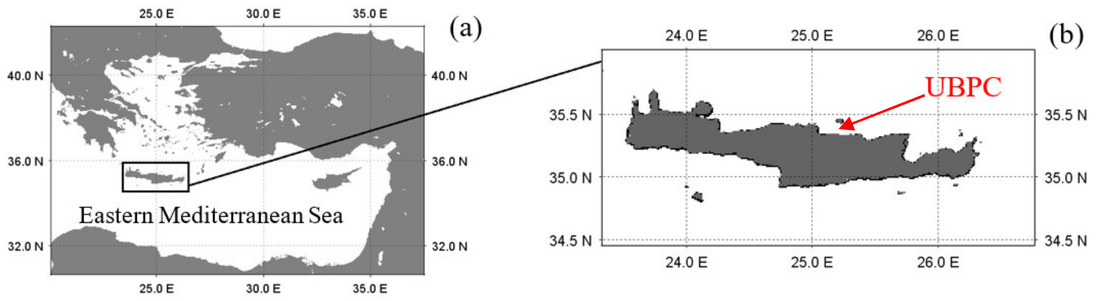
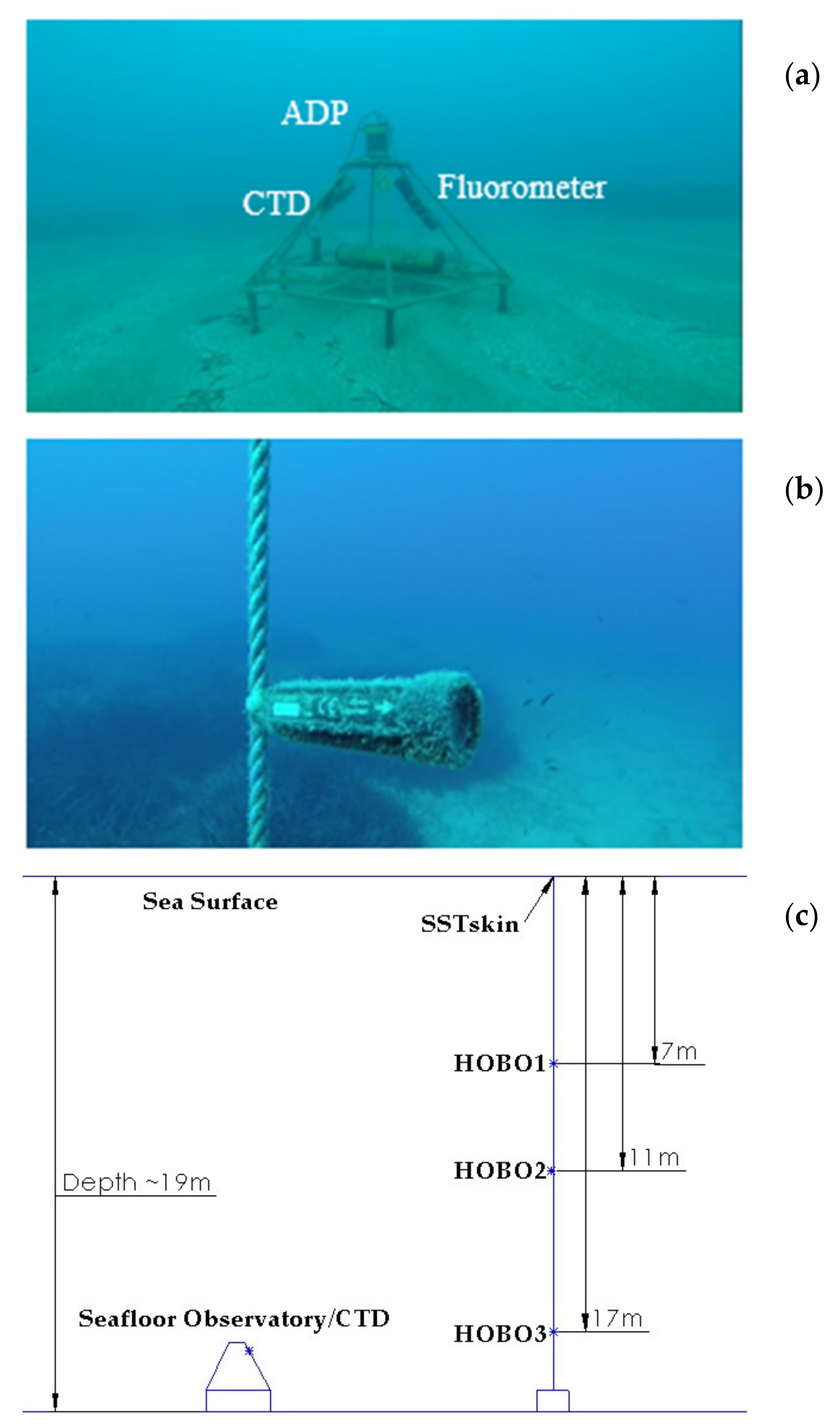
In this study, a similar method to Brewin et al. [21] was followed, where in situ temperature data recorded in the Underwater Biotechnological Park of Crete (UBPC) were compared with satellite SST data from MODIS Aqua and MODIS Terra instruments. The UBPC is a unique resource in the Eastern Mediterranean since it is a large-scale in situ research infrastructure in the coastal zone of Crete that provides autonomous temperature recordings since 2014. The UBPC started as a biotechnology multi-use infrastructure and the instruments that were installed therein were for the needs of the local environmental monitoring. However, because of the shallow nature of the temperature monitoring installations, and since the location of the UBPC is in a key-spot of biodiversity changes due to Lessepsian Migration and may be prone to climatic changes [35,36,37], it was thought this time series could also potentially be useful for satellite coastal SST validation, and thus, it was decided to exploit the vertical temperature loggers four-year time series for a comparison with the MODIS Aqua and Terra SST data.

In this study, the main aim was therefore to evaluate the data collected from the autonomous in situ data loggers of the UBPC for use in the validation of near-shore satellite SST measurements. The hypothesis that the UBPC data could be useful in this way was tested by correlating the in situ data with MODIS SST satellite data and examining the possible errors and biases related to such factors as instrumentation and proximity to the shore.

2. Methods

2.1. Study Area

In the framework of various research projects of the Institute of Marine Biology, Biotechnology and Aquaculture of the Hellenic Centre for Marine Research (HCMR), the Underwater Biotechnological Park of Crete (UBPC) has been developed. The UBPC is a unique large-scale in-situ research infrastructure that covers an area of 0.03 km², lies about 2 km offshore the northern Cretan coast in the vicinity of the HCMR land premises in Crete, with a depth increasing from 18 to 22 m along a south–north direction. Objectives of the UBPC are the protection, conservation, and exploitation of marine biological resources, the development of innovative technologies in the fields of open sea invertebrate aquaculture, and marine ecotourism including the development of the HCMR Artificial Reefs^© and long-term monitoring of the coastal environment. In May 2014, a bottom moored seafloor observatory was deployed that was comprised of various scientific instruments mounted on a metal truss construction. The seafloor observatory is equipped with an Acoustic Doppler Profiler (ADP, for the measurement of sea current velocity/direction in the water column and wave velocity and height), a Fluorometer (for the measurement of in-vivo chlorophyll-a, turbidity, and fluorescence) and a conductivity-temperature-density instrument (CTD, for the continuous measurement of sea temperature, salinity, density, sound velocity, and dissolved oxygen). Alongside the seafloor observatory, a vertical temperature logger array is deployed that has six sensors equally spaced from 7 m down to 17 m depth.

2.2. In Situ Temperature Datasets

2.2.1. Seafloor Temperature Dataset from CTD

In May 2014, the SAIV SD208 CTD sensor was deployed with the seafloor observatory at a depth of approximately 19 m in the southwest sector of the UBPC (Figure 1, latitude = 35.346621O N, longitude = 25.278761O E). According to the manufacturers specifications, the instrument is certified for an accuracy of +/−0.003 °C, over a range of −2 to 40 °C, with a resolution of 0.0002 °C and a response time of 0.1 s. The instrument is accompanied by a Calibration Certificate (no. 3065) by Sensordata a.s. and SAIV A/S, Bergen, Norway that gives a traceable reference of a General Oceanics ATB 1250 temperature bridge with serial number 1235 and takes as working reference a Falmouth (Cataumet, MA, USA) Scientific Model OTM S-112 S/N 1377-09JUL96 instrument [38]. The SAIV SD208 CTD manual states that ‘Due to the excellent long term stability of sensors and circuitry, the instrument does not have to be recalibrated for several years.’ The initial sampling/recording interval was set to 5 min. The position of the instrument is approximately 1.5 m from the seafloor (Figure 2a). Every 3–6 months over the duration of this study, the SAIV CTD was retrieved by scuba divers for the cleaning and maintenance of its sensors and data were downloaded using the SAIV-MINISOFT SD200W software (SAIV A/S, Bergen, Norway). This software serves as the communication with the instrument to set it up and download and process the recorded data. Operational difficulties, due to bad weather conditions, sometimes prevented the scientific diving team of HCMR to redeploy the instruments immediately after the maintenance processes, thus, leading to some short periods of data gaps. The number and periods of data collected are presented in

Table A1. Period of deployment for every sensor in the Underwater Biotechnological Park of Crete.

Sensor	Year	Period
CTD	2014	26/05/2014–31/12/2014
	2015	01/01/2015–31/12/2015
	2016	01/01/2016–02/10/2016 & 07/12/2016–31/12/2016
	2017	01/01/2017–31/12/2017
	2018	01/01/2018–27/03/2018
HOBO1	2014	14/07/2014–31/12/2014
	2015	01/01/2015–31/12/2015
	2016	01/01/2016–07/06/2016 & 09/12/2016–31/12/2016
	2017	01/01/2017–31/12/2017
	2018	01/01/2018–01/11/2018
HOBO2	2014	14/07/2014–31/12/2014
	2015	01/01/2015–31/12/2015
	2016	01/01/2016–07/06/2016 & 09/12/2016–31/12/2016
	2017	01/01/2017–22/08/2017
	2018	27/03/2018–01/11/2018
HOBO3	2014	16/10/2014–31/12/2014
	2015	01/01/2015–31/12/2015
	2016	01/01/2016–07/06/2016 & 09/12/2016–31/12/2016
	2017	01/01/2017–31/12/2017
	2018	01/01/2018–01/11/2018

alongside the data series of the accompanying sensors for this study.

2.2.2. Water Column Temperature Dataset from HOBO Array

In August 2014 a HOBO Water Temp Pro v2 U22-001 (Onset Computer Corporation, Bourne, MA, USA) (Figure 2b) vertical sensor array was deployed approximately 10 m from the seafloor observatory of the UBPC (Figure 2c). According to the manufacturer’s specifications, a HOBO sensor is certified for an accuracy of +/−0.21 °C, over a range of 0 to 50 °C, with a resolution of 0.02 °C and response time of 5 min in water. The initial sampling/recording interval was therefore set to 10 min. The vertical HOBO array expands from 7 to 17 m below the sea surface and consists of six equally spaced sensors—one every 2 m—mounted on a floating rope with buoys and weights to keep the sensors location in the water column precise. The deepest sensor is approximately 1.5 m above the seafloor, thus, differing in depth less than 1 m from the CTD of the seafloor observatory. Every 6–12 months over the duration of this study, the HOBO sensors data were downloaded by SCUBA divers using the HOBO Waterproof Shuttle for the readout and relaunching the HOBO sensors. The HOBO Waterproof Shuttle is compatible with HOBO data loggers having an Optic USB interface and is waterproof to 20 m, with an operating temperature ranging from 0 to 50 °C. For safety reasons, the deepest HOBO sensor was placed 2–3 m above the 20 m operational limit of the HOBO Waterproof Shuttle. Twice during the duration of this study, the whole HOBO sensor array was retrieved by the scientific diving team of HCMR for the cleaning and maintenance of its sensors. The first time was for the replacement of the sensors and the second time due to their batteries running out. During these two retrievals, data were downloaded with the same HOBO Waterproof Shuttle. After every download, HOBOware Pro software (Onset Computer Corporation, Bourne, MA, USA) was used for data readout and processing and to set up each HOBO sensor. From 2014 to 2016, a sampling/recording interval of 10 min was selected. From 2016 to 2018, the sampling interval was changed to 30 min to expand the battery life of the sensors.

For this study, data from three HOBO sensors were used. The first dataset is from the sensor located 7 m below sea surface, the second dataset is from the sensor located 11 m below sea surface, the third dataset is from the sensor located 17 m below sea surface, hereafter called HOBO1, HOBO2, and HOBO3, respectively. The number and periods of data collected are presented in Table A1 alongside the accompanying CTD data series for this study.

2.3. Remote Sensing SST Datasets

Remote sensing SST data were provided by the NASA Goddard Space Flight Center, Ocean Ecology Laboratory, Ocean Biology Processing Group and downloaded from NASA’s OceanColor website (https://oceancolor.gsfc.nasa.gov/). For this study, MODIS level 2 datasets were downloaded. MODIS is an instrument onboard the Aqua and Terra satellites that views the entire Earth’s surface every 1 to 2 days and acquires data in 36 spectral bands with a swath of 2330 km by 10 km along track at nadir. The spatial resolution of the MODIS instrument for the bands that correspond to the datasets used in this study is 1 × 1 km. Remote sensing datasets of SST and SST4 (night time SST at 4 μm wavelength), which refer to skin measurements (a thin layer of ~500 μm depth at the water side of the air-sea interface), were downloaded in netcdf format for the period of May 2014 until October 2018, hereafter referred to as AQUASST/AQUASST4 and TERRASST/TERRASST4, respectively.

Algorithms were designed to extract the appropriate data. Firstly, the cell of each Aqua and Terra MODIS swath that contained the coordinates of the Seafloor Observatory (35.346621° N, 25.278761° E) was selected and then only the data with a quality flag of ≤2 were used for the next steps of the analysis. These quality flags are used to select valid SST data and have five possible values as defined in NASA’s MODIS documentation: 0—best quality, 1—good quality, 2—suspect, 3—bad (cloud/ice/dust or atmospheric correction failed), 4—product failure (not processed or land). Furthermore, the northern adjacent data cell for each of the previously selected cells was extracted, in order to compare the values between them, since the northern cell lies further offshore from the coast and allowed the possible effects of land adjacency and signal contamination to be examined. The data corresponding to the northern adjacent cell in each case will be referred to as AQUASST_N/AQUASST4_N and TERRASST_N/TERRASST4_N, with the same pattern as the data from the cell containing the seafloor observatory.

2.4. Data Processing and Analysis

All the data recorded from the in situ loggers were initially set to the Local Time Zone—UTC +2 (EET) and UTC +3 (EEST)—but for the needs of this study time data were transformed to GMT to equate to the units of the Aqua and Terra satellite data. Then, a comparison between the CTD and the HOBO3 data took place to examine any differences between the two instruments that measure water temperature at the same depth (~17 m). This was necessary because of the lack of any certificate of calibration for the HOBO sensors, and thus, the calibration certificate of the CTD was used to provide a rough check on the measurement accuracy of the HOBOs in their long-term deployment conditions. Following this equivalence check, a comparison between the HOBO1, HOBO2, and HOBO3 datasets took place, to see any differences in the water column temperature. HOBO1 nighttime data were extrapolated to surface following the Group for High Resolution Sea Surface Temperature (GHRSST) [39] method recommended by Donlon et al. [40]. In this study, the relationship between nighttime temperature from 5 m depth and surface temperature, for wind speeds greater than 2 m/s, was formulated [40] Equation (2). Data computed for generating their formula were recorded in various research expeditions using above water infrared radiometers and in water thermistors and refer to approximately 5 m depth. However, Donlon et al. [40] suggested that this extrapolation method is applicable for the upper ocean layer to ~10 m depth, if well mixed, making it suitable for our 7 m depth bulk temperature measurements. Thus, only nighttime in situ data for wind speeds >2 m/s were extrapolated and used in this study, to avoid the complicating effect of diurnal stratification, according to the aforementioned method. This extrapolated dataset, which was compared with satellite measurements, will be referred to as SSTskin. Finally, the remote sensing datasets AQUASST4 and TERRASST4 were compared to the SSTskin dataset for validation potential, and all remote sensing datasets were compared between each other to see any differences due to distance from the coastline. For the comparison between the SSTskin and the remote sensing data series, only the in situ data that were logged one hour before or after the satellite overpass were selected. For this study, up to 12 in situ data values were averaged and compared with the remote sensing data values (i.e., 1 h either side of the satellite overpass time with a 10-min sampling rate). For all datasets descriptive statistics (e.g., mean value, standard deviation-StD, standard error-SE, range-Min/Max, number of days with valid data-N) were compiled, and for each comparison between datasets, a set of correlation and bias statistics were calculated (e.g., squared Pearson correlation coefficient-r², mean bias-δ, mean absolute error-Δ, root mean squared error-Ψ).

3. Results

3.1. Comparison between In Situ Temperature Data

3.1.1. Comparison between the CTD and the HOBO3 Data

For this study to be as efficient as possible in terms of calibration and accuracy, a comparison between the SAIV CTD temperature sensor and the HOBO3 temperature logger took place. The SAIV CTD was accompanied with a Certificate of Calibration with traceable references of instrumentation [38]. Since the two instruments were deployed at nearly the same depth (CTD at ~17.5 m and HOBO3 at ~17 m), their data were compared for the whole duration of this study. In Figure 3, the data series of the CTD and the HOBO3 is presented, and in

Table 1. Comparison statistics between the CTD, the HOBO1, the HOBO2, and the HOBO3 datasets. The squared Pearson correlation coefficient (r²), the mean bias (δ), the mean absolute error(Δ), the root mean squared error (Ψ), and the number of matchups taken into account (N) are presented for daily averaged values. The last column refers to the percentage of the raw data matchups—not the daily averaged—that had difference over >2 °C / >3 °C, respectively.

	r2	δ	Δ	Ψ	N	% of Matchups with Difference >2 °C/>3 °C
HOBO3–CTD	0.9970	0.06	0.12	0.21	1066	-
HOBO1–HOBO2	0.9987	0.05	0.16	0.16	1170	0.004%/0%
HOBO1–HOBO3	0.9916	0.13	0.18	0.40	1292	1.17%/0.33%
HOBO2–HOBO3	0.9952	0.11	0.13	0.30	1076	0.53%/0.06%

, the statistics of their recorded data are presented. Figure 3a shows a good agreement between the two data series over time and in Figure 3b, the difference between the HOBO3 minus the CTD is presented. Figure 3c shows the correlation plot for this comparison with correlation statistics. The squared Pearson’s correlation coefficient was 0.9970, which was calculated from 1066 days of recordings where both instruments were deployed with their daily averaged values taken into account. The mean bias was calculated to be δ = 0.063 °C and the mean absolute error Δ = 0.1178 °C (Table 1). The correlation statistics show that the HOBO3 temperature measurements were in good agreement with the CTD measurements. However, if one assumes that they were both measuring a uniformly well-mixed water mass, and if the CTD is considered “truth,” then the HOBO3 had a measurement bias of ~0.1–0.2 °C (depending on the bias parameter used). This is in keeping with the stated accuracy of the instrument and is also within the established uncertainty level of thermistors on drifting buoys (0.2 K) calculated from three-way analysis methods [41,42,43].

Furthermore, the mean annual (Mean), the standard deviation (Std), the standard error (SE), the minimum (Min), and the maximum (Max) values for every sensor were calculated and are presented in

Table A2. Statistical data extracted from daily averaged values of the deployed instruments in the Underwater Biotechnological Park of Crete, and the corresponding days of measurement for every year. Interannual variations occur due to different periods of deployment from year to year (see Table A1). The mean value of daily averaged data, the standard deviation, the standard error, the minimum, and maximum values for each data series are presented.

Sensor	Year	Mean	StD	SE	Min	Max	Days
CTD	2014	23.2651	2.7996	0.194586	17.9808	27.3790	207
	2015	20.6792	3.9237	0.205658	15.0753	27.7596	364
	2016	20.5336	4.1066	0.237095	15.4409	27.2247	300
	2017	20.4080	3.9063	0.204465	14.4606	27.0765	365
	2018	16.1836	0.4254	0.045872	15.5002	17.3387	86
HOBO1	2014	23.5580	3.1856	0.245046	16.0967	27.7329	169
	2015	20.8872	4.0666	0.212856	14.9445	28.1352	365
	2016	17.6343	1.5589	0.115553	15.7778	22.3708	182
	2017	20.6020	4.0199	0.210411	14.3907	27.4004	365
	2018	21.4671	4.3554	0.249389	14.0752	27.6611	305
HOBO2	2014	23.5674	3.1649	0.243454	16.1505	27.8156	169
	2015	20.8691	4.0223	0.210537	15.0354	27.8438	365
	2016	17.6100	1.5093	0.111877	15.7806	22.3003	182
	2017	19.8281	4.3129	0.281943	14.4217	27.2163	234
	2018	23.3735	3.3278	0.22436	16.1800	27.5739	220
HOBO3	2014	20.3626	1.7853	0.206149	15.3942	23.6355	75
	2015	20.7576	3.9212	0.205245	15.0493	27.7035	365
	2016	17.5311	1.4586	0.108119	15.5188	22.1203	182
	2017	20.4538	3.9013	0.204203	14.4756	27.1492	365
	2018	21.3070	4.2799	0.245066	15.5077	27.5616	305

alongside the days of deployment per year for every sensor. Variations in the aforementioned values (e.g., HOBO1 2014 vs. HOBO1 2015) are not anomalies but have to do with the different periods within the year that each sensor was deployed (refer to Table A1). For annual datasets that cover most days of the year, such as CTD 2015 and CTD 2017 or HOBO3 2015 and HOBO3 2017, there is a common temperature pattern with an average value of approximately 20.5 °C and a standard deviation of approximately 4 °C.

3.1.2. Comparison between the HOBO1, HOBO2, and HOBO3 Data

The HOBO1, HOBO2, and HOBO3 loggers are part of a vertical array that is located 10 m away from the Seafloor Observatory and was initially deployed to record any variations in water column temperature and investigate any correlation with sea current velocity and direction (acquired by the ADP). For the needs of this study, the temperature variations due to different depths were examined, in order to examine any depth related biases concerning the vertical mixing of our study area.

In Figure 4a the temperature time series of the HOBO1 and the HOBO2 loggers is presented. The datapoints present the daily averaged data for each logger and only days that both sensors were recording were taken into account. The difference between HOBO1 minus HOBO2 is presented in Figure 4b. In Figure 4c, the correlation plot between HOBO1 and HOBO2 daily averaged values is presented. The squared Pearson’s correlation coefficient was 0.9987 and the average temperature difference for the whole time series was 0.0456 °C. The number of days that both sensors were recording was 1170. It was expected that the temperature difference between the HOBO1 minus the HOBO2 data was going to be slightly positive, as these results show, because HOBO1 is deployed at 7 m below the sea surface, while HOBO2 is deployed 11 m below the sea surface.

In Figure 5a, the temperature time series of the HOBO1 and the HOBO3 loggers is presented. The datapoints present the daily averaged data for each temperature logger and again only days that both sensors were recording were taken into account. In Figure 5c, the correlation plot between HOBO1 and HOBO3 daily averaged values is presented. The squared Pearson’s correlation coefficient is 0.9916 and the average temperature difference for the whole time series is 0.1332 °C. The days that both sensors were recording were 1292. It was expected that the temperature difference between the HOBO1 minus the HOBO3 data was going to be positive, as these results show (Figure 5b, δ = 0.13 °C), because the HOBO1 is deployed at 7 m below the sea surface, while HOBO3 is deployed 17 m below the sea surface and ~1.5 m above the seafloor.

As Table 1 presents, there is a small percentage of matchups that have a difference of >2 °C and >3 °C between the HOBO sensors data. This means that under most conditions, the study area is vertically well-mixed. However, as presented in Figure 4b and Figure 5b there are periods that temperature differences of more than 2 °C—up to 3 °C—can happen especially when comparing the shallowest HOBO1 (7 m) with the deepest HOBO3 (17 m) dataset. These differences were recorded during summertime, a fact that is possibly due to clear hotter sunny days with light currents and wind, resulting in increased direct sunlight heating the closer to the surface HOBO1 logger.

Furthermore, for local environmental monitoring, CTD casts have been undertaken in the vicinity of the seafloor observatory since its installation at various times of year, covering all four seasons (results not shown). These have always shown a good correlation with the HOBO sensors at their specific depths, thus, adding further support to the hypothesis that the study area is vertically well-mixed.

3.2. Comparison between In Situ and Remote Sensing Temperature Data

In this section, the results associated with the data recorded in the cell that contains the Seafloor Observatory location are presented.

Table A3. Statistical data extracted from remote-sensing satellite measurements with quality flag values of 0, 1, and 2. The mean value, the standard deviation, the standard error, the minimum, and maximum values for each data series are presented. Additionally, the number of days that had the corresponding quality flag values for every year is presented. Data series with the ‘_N’ ending refer to the northern cell of the satellite swath from the cell that contains the Seafloor Observatory of the Biotechnological Park of Crete.

Sensor	Year	Mean	StD	SE	Min	Max	Days
AQUASST	2014	23.4166	3.5380	0.505429	16.2250	27.4900	49
	2015	23.5043	3.6787	0.554585	15.8900	29.9450	44
	2016	22.8998	3.3402	0.427669	16.3550	28.8200	61
	2017	22.8295	4.1823	0.563941	14.5800	27.0400	55
	2018	25.2624	2.2572	0.301631	16.5900	27.6850	56
AQUASST4	2014	23.5379	3.2620	0.639731	16.7000	27.1550	26
	2015	24.0261	3.2073	0.617245	16.3850	28.8450	27
	2016	23.2771	3.2781	0.642888	17.4700	27.1550	26
	2017	23.6767	3.1903	0.713373	16.4550	26.4850	20
	2018	25.3684	2.8590	0.5718	16.7300	27.6600	25
TERRASST	2014	22.5046	3.8579	0.42346	12.1800	27.4400	83
	2015	23.4049	3.8319	0.436686	14.6950	28.6600	77
	2016	22.8998	3.3402	0.427669	16.3550	28.8200	61
	2017	22.8295	4.1823	0.563941	14.5800	27.0400	55
	2018	23.1479	4.1998	0.491549	14.4050	27.9300	73
TERRASST4	2014	22.5683	3.9895	0.59472	15.4100	27.7850	45
	2015	23.9990	3.8150	0.545	15.8250	29.2050	49
	2016	23.2771	3.2781	0.642888	17.4700	27.1550	26
	2017	23.6767	3.1903	0.713373	16.4550	26.4850	20
	2018	24.0743	3.8630	0.507237	15.6000	28.0150	58
AQUASST_N	2014	23.3129	3.5346	0.510176	16.1050	27.4100	48
	2015	23.4441	3.4335	0.542884	15.7800	29.7650	40
	2016	22.9784	3.3350	0.437907	16.2700	28.6000	58
	2017	22.7984	4.2106	0.627679	14.5950	27.0400	45
	2018	25.3579	2.3345	0.336956	16.4750	27.5100	48
AQUASST4_N	2014	23.3467	3.3631	0.659558	16.2850	27.1750	26
	2015	24.0608	2.8468	0.56936	17.3750	28.6800	25
	2016	23.3600	3.2674	0.6813	17.4200	27.1400	23
	2017	23.4629	3.1871	0.731171	16.5150	26.5750	19
	2018	25.0714	2.8814	0.614317	16.6900	27.5350	22
TERRASST_N	2014	22.2908	3.8583	0.445518	12.1650	27.3250	75
	2015	23.4556	3.7451	0.447625	14.8900	28.7600	70
	2016	22.9784	3.3350	0.437907	16.2700	28.6000	58
	2017	22.7984	4.2106	0.627679	14.5950	27.0400	45
	2018	22.7552	4.3419	0.560537	14.5200	27.4750	60
TERRASST4_N	2014	22.3801	3.9640	0.626763	15.6400	27.4450	40
	2015	23.8145	3.9018	0.575289	15.9800	28.7150	46
	2016	23.3600	3.2674	0.6813	17.4200	27.1400	23
	2017	23.4629	3.1871	0.731171	16.5150	26.5750	19
	2018	23.6804	3.9737	0.573554	16.0700	27.6750	48

presents the annual average value, the standard deviation (StD), the standard error (SE), the minimum (Min), and maximum (Max) values recorded and the number of days that a satellite overpass with quality flag values of 0, 1, and 2 occurred. Data in Table A3 refer to every satellite SST dataset of AQUASST, AQUASST4, TERRASST, and TERRASST4.

AQUASST4 data are presented in Figure 6a, with the averaged SSTskin data from within ±1 h from the respective satellite overpass, resulting in a good matchup that follows a sinusoidal interannual SST pattern. In Figure 6c, the correlation plot between AQUASST4 and SSTskin data is presented, where the squared Pearson’s correlation coefficient is 0.9847 from 92 mutual pairs of measurements.

To evaluate the utilization of the Terra MODIS SST data, the same selection of cells and the same filtering and processing as the Aqua MODIS SST data took place. The acquired TERRASST4 dataset is presented in Figure 7a compared with the averaged SSTskin data that were obtained within ±1 h of the respective satellite overpass. Again, the results show a good matchup, following a sinusoidal interannual SST pattern. In Figure 7c the correlation plot between TERRASST4 and SSTskin data is presented and the squared Pearson’s correlation coefficient is 0.9689, from 90 mutual pairs of measurements (

Table 2. Comparison statistics between the MODIS AQUA and MODIS TERRA datasets and the SSTskindata. The SSTskin data are averaged from within +/−1 h of the AQUA and TERRA satellite overpass. The squared Pearson correlation coefficient (r²), the mean bias (δ), the mean absolute error (Δ), the root mean squared error (Ψ), and the number of matchups taken into account are presented.

	r2	δ	Δ	Ψ	N
SSTskin–AQUASST4	0.9847	−0.08	0.27	0.42	92
SSTskin–TERRASST4	0.9689	−0.35	0.51	0.76	90

).

3.3. Comparison between the MODIS Aqua and Terra Data from the Cell Containing the Seafloor Observatory of the Underwater Biotechnological Park of Crete and the Northern Adjacent Cell

For the purpose of examining land contamination of the satellite remote sensing SST data due to the proximity of the coastline with the site of this study, for each of the MODIS datasets the northern adjacent cell to the one that contains the Seafloor Observatory was extracted and the respective temperature value was selected, thus creating the AQUASST_N, AQUASST4_N, TERRASST_N, and TERRASST4_N datasets. The new datasets were treated with the exact algorithms as the datasets of the cell containing the Seafloor Observatory location. The extracted MODIS Aqua and MODIS Terra data with value flags of 0, 1, and 2 are compared with the respective ones that are extracted from the cell containing the in situ loggers. Table A3 presents the annual average value, the standard deviation (StD), the standard error (SE), the minimum (Min), and maximum (Max) values recorded and the number of days that a satellite overpass with quality flag values of 0, 1, and 2 occurred. Data in Table A3 refer to every satellite SST dataset of AQUASST_N, AQUASST4_N, TERRASST_N, and TERRASST4_N.

All data pairs under comparison have the same sampling time, since they are collected from the same satellite swath. First, a comparison from the MODIS Aqua dataset is presented in Figure 8 and Figure 9, referring to SST (daytime) and SST4 (nighttime) data, respectively. Both comparisons result in high comparison statistics, with data following a sinusoidal interannual pattern (Figure 8a and Figure 9a) and most matchups have a difference less than 0.5 °C (Figure 8b and Figure 9b). In Figure 8c and Figure 9c, the correlation plot between the loggers’ cell and the northern adjacent cell is presented for the daytime and the nighttime satellite measurements, respectively. The squared Pearson’s correlation coefficient is 0.995 and the mean bias is 0.02 for 199 pairs of data of daytime MODIS Aqua measurements (Figure 8c). For the nighttime MODIS Aqua, the squared Pearson’s correlation is 0.9947 and the mean bias is 0.07 for 92 pairs of data (Figure 9c).

Similar to the MODIS data from the cell containing the Seafloor Observatory location, in order to evaluate the utilization of the Terra MODIS SST data, the same selection of cells and the same filtering and processing as with the AQUASST_N and AQUASST4_N data took place. The acquired TERRASST_N and TERRASST4_N datasets are presented in Figure 10 and Figure 11. Again, the data result in a good matchup and follow a sinusoidal interannual SST pattern (Figure 10a, Figure 11a). Most of the differences between the two adjacent cells were less than 0.5 °C both for daytime and nighttime satellite measurements (Figure 10b, Figure 11b). The squared Pearson’s correlation coefficient was 0.995 for the daytime matchups and 0.9945 for the nighttime matchups. The mean bias for both the daytime data and the nighttime data was δ = 0.03. The above were calculated from 135 and 87 pairs of daytime and nighttime data, respectively (

Table 3. Comparison statistics between the RS SST values from the cell containing the in situ data loggers and its northern adjacent cell, both for the MODIS AQUA and the MODIS TERRA datasets. The squared Pearson correlation coefficient (r²), the mean bias (δ), the mean absolute error (Δ), the root mean squared error (Ψ), and the number of matchups taken into account are presented.

	r2	δ	Δ	Ψ	N
AQUASST–AQUASST_N	0.9950	0.02	0.20	0.26	199
AQUASST4–AQUASST4_N	0.9947	0.07	0.19	0.26	92
TERRASST–TERRASST_N	0.9950	0.03	0.23	0.30	135
TERRASST4–TERRASST4_N	0.9945	0.03	0.22	0.28	87

).

4. Discussion

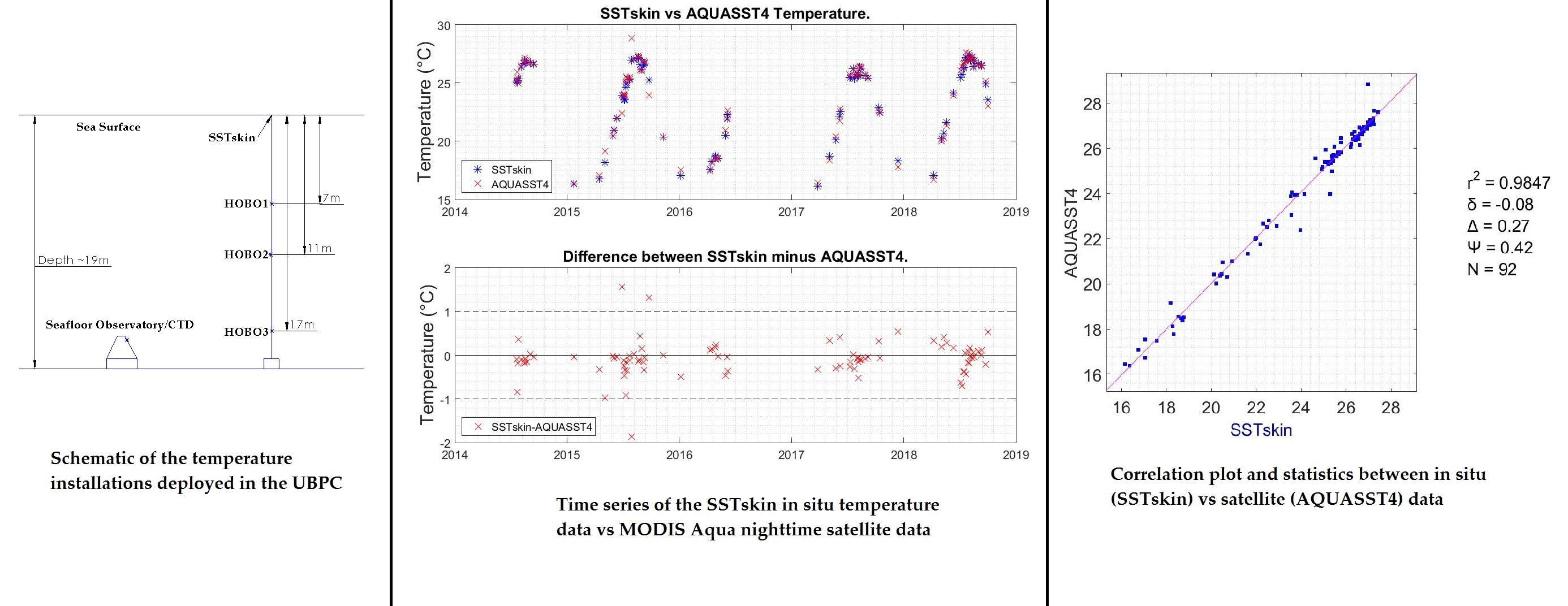
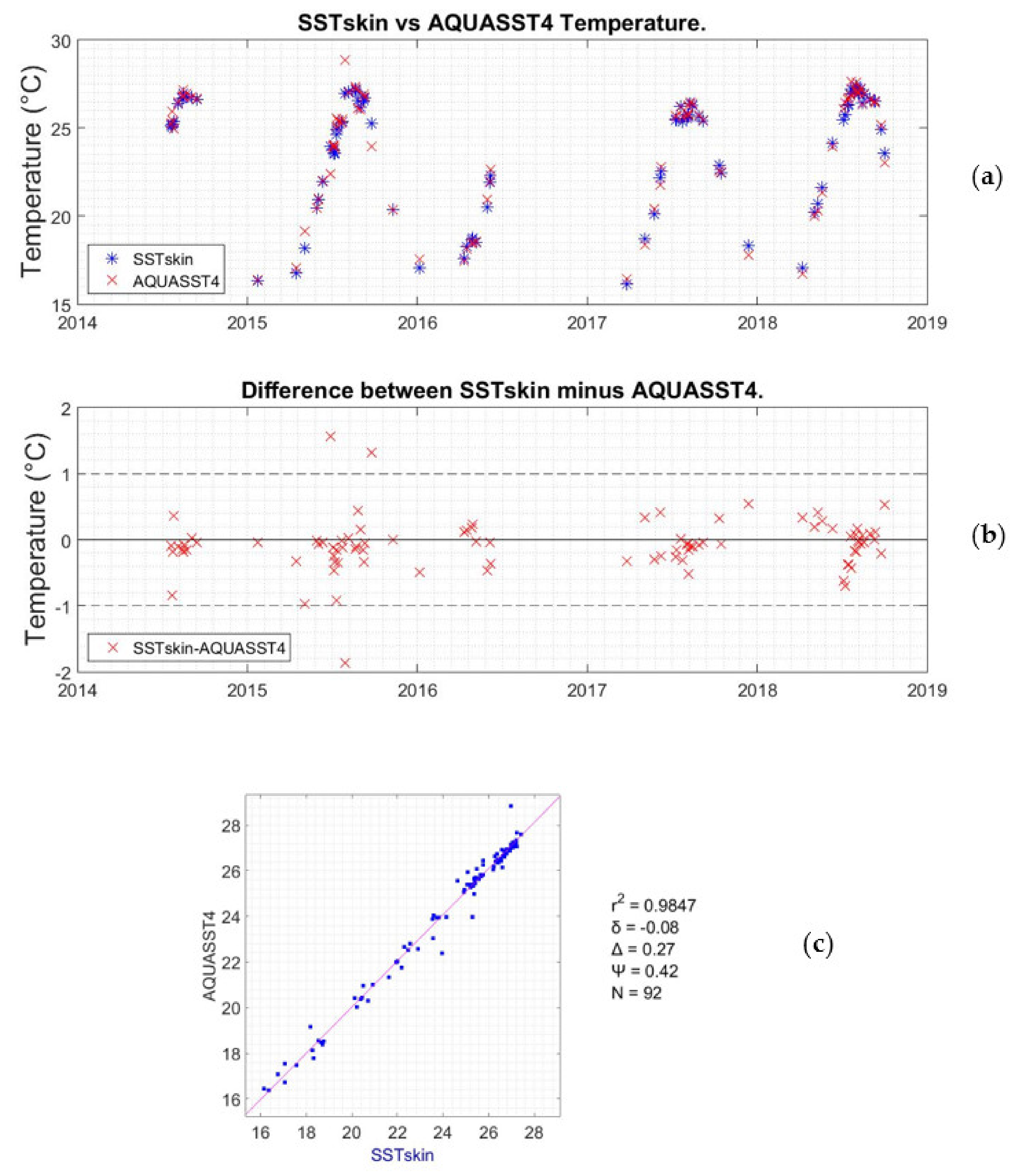
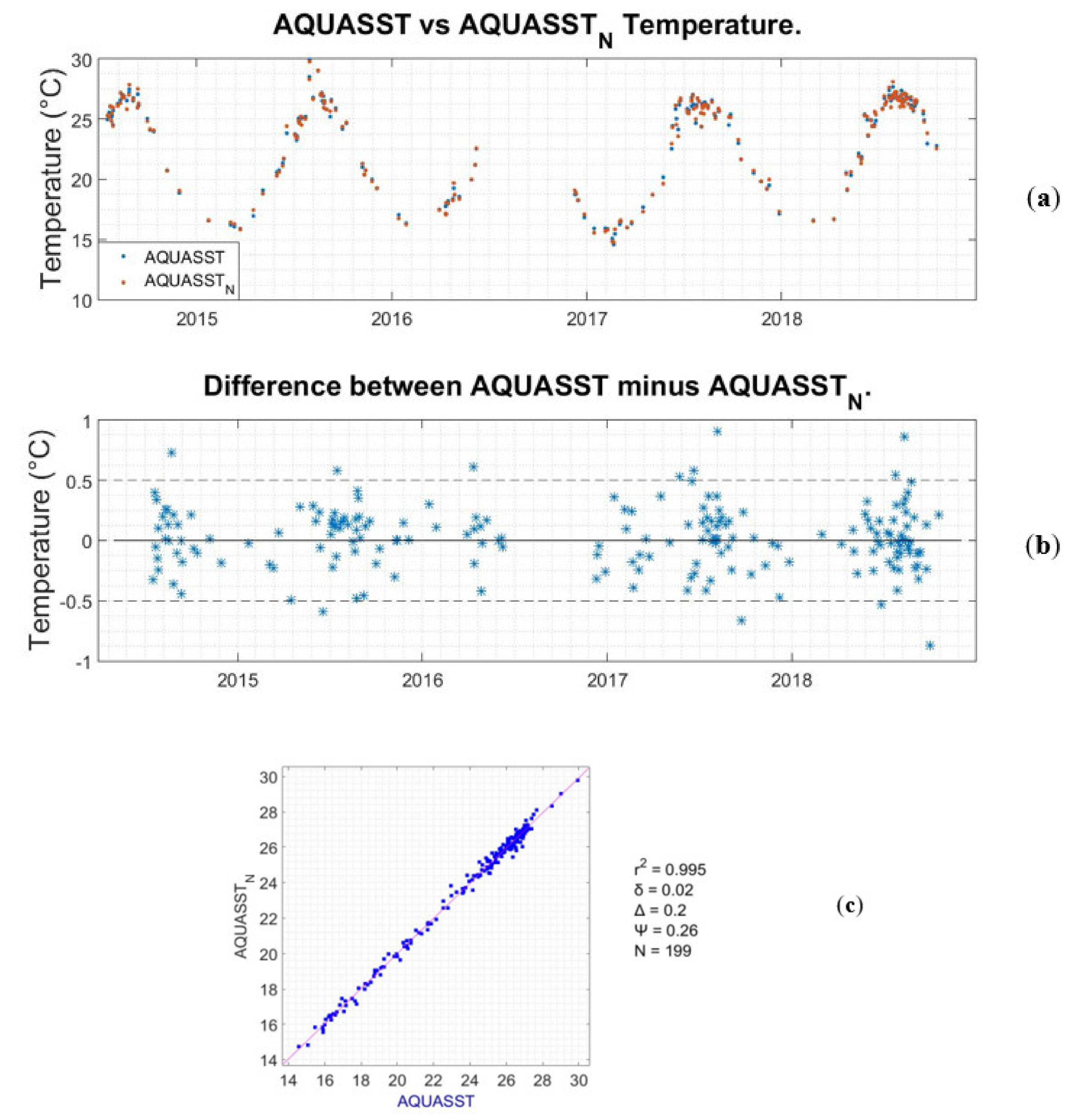
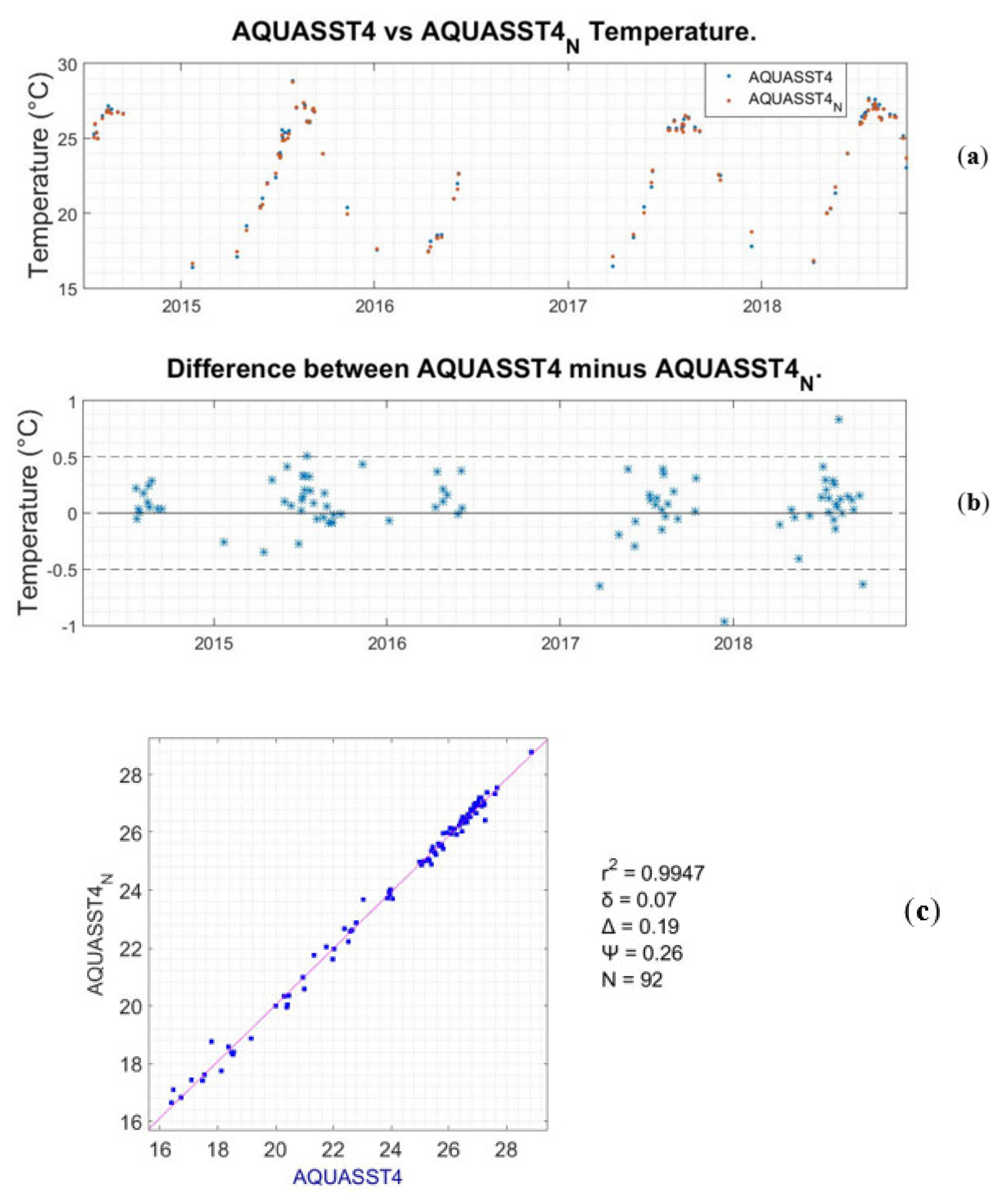
This study utilized the four-year data series of the in situ temperature loggers deployed in the Underwater Biotechnological Park of Crete and investigated the data’s suitability for use in the validation of MODIS SST products. 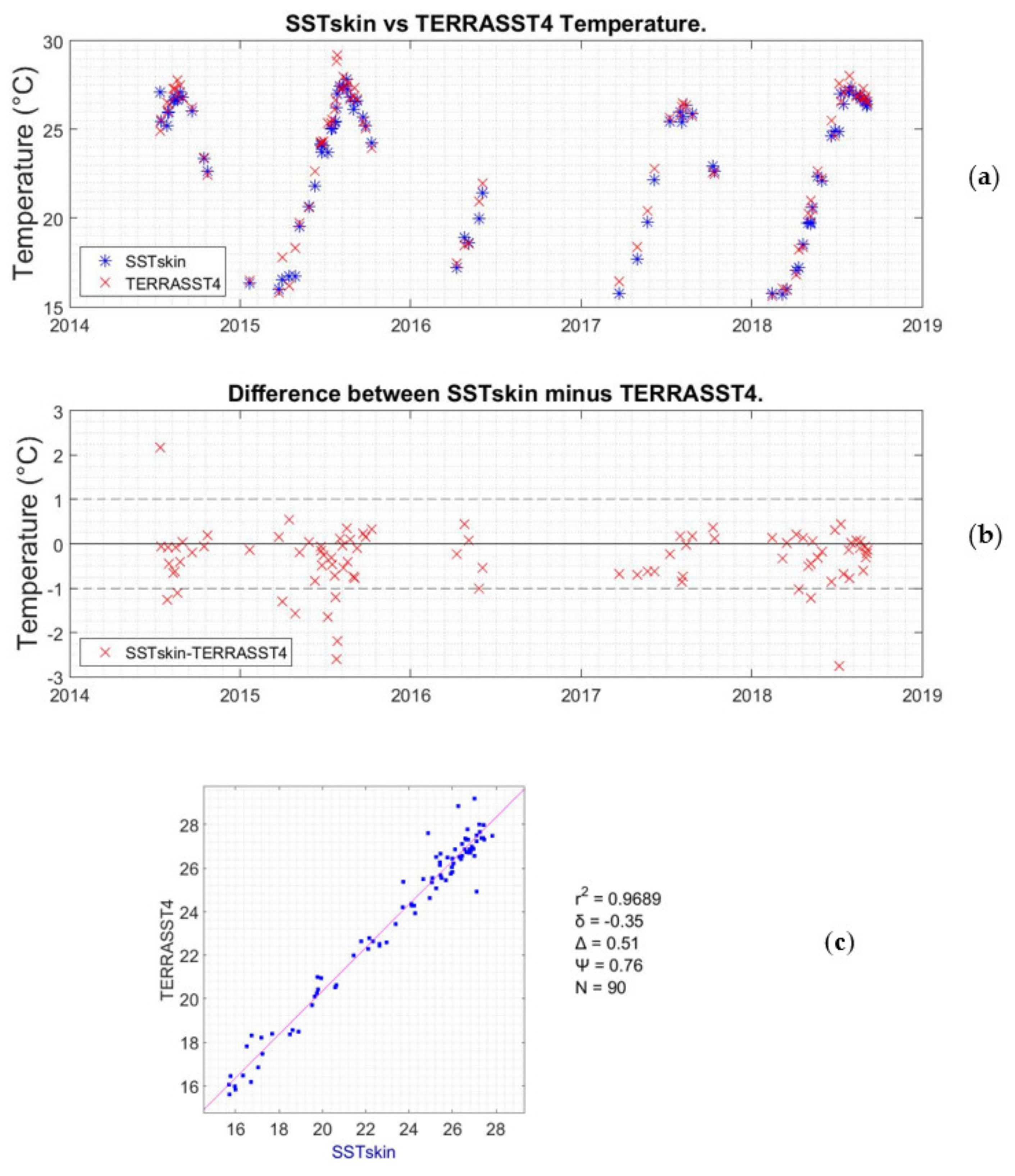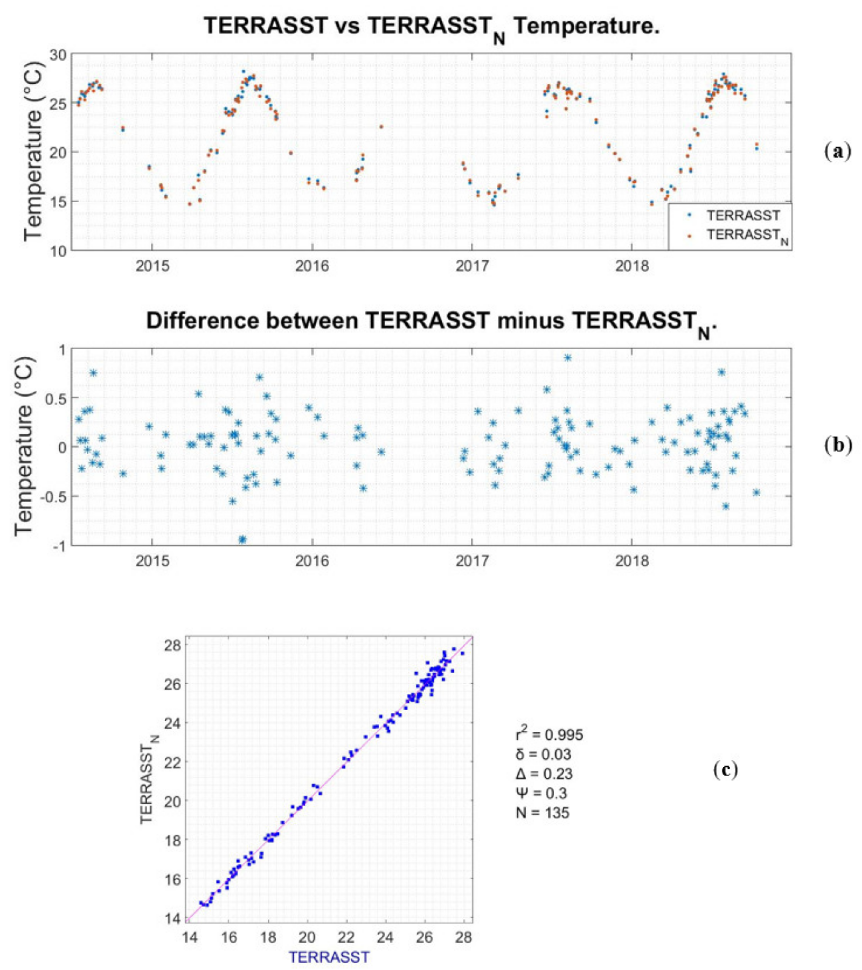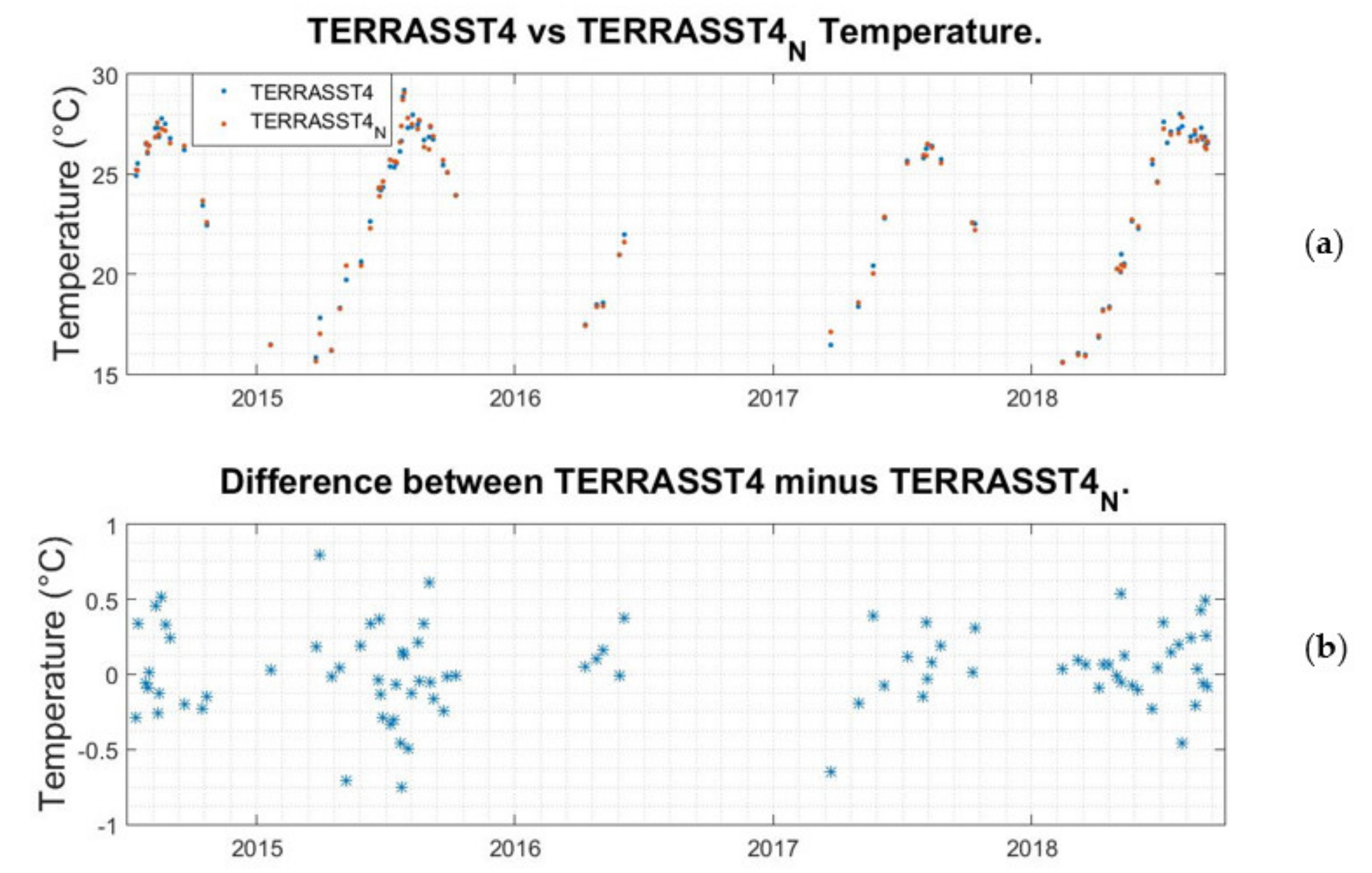For the in situ SSTskin, when compared with the AQUASST4 data, there was a negative bias with mean bias values (δ) of −0.08 and squared Pearson’s correlation coefficient equal to 0.9847 (Table 2). 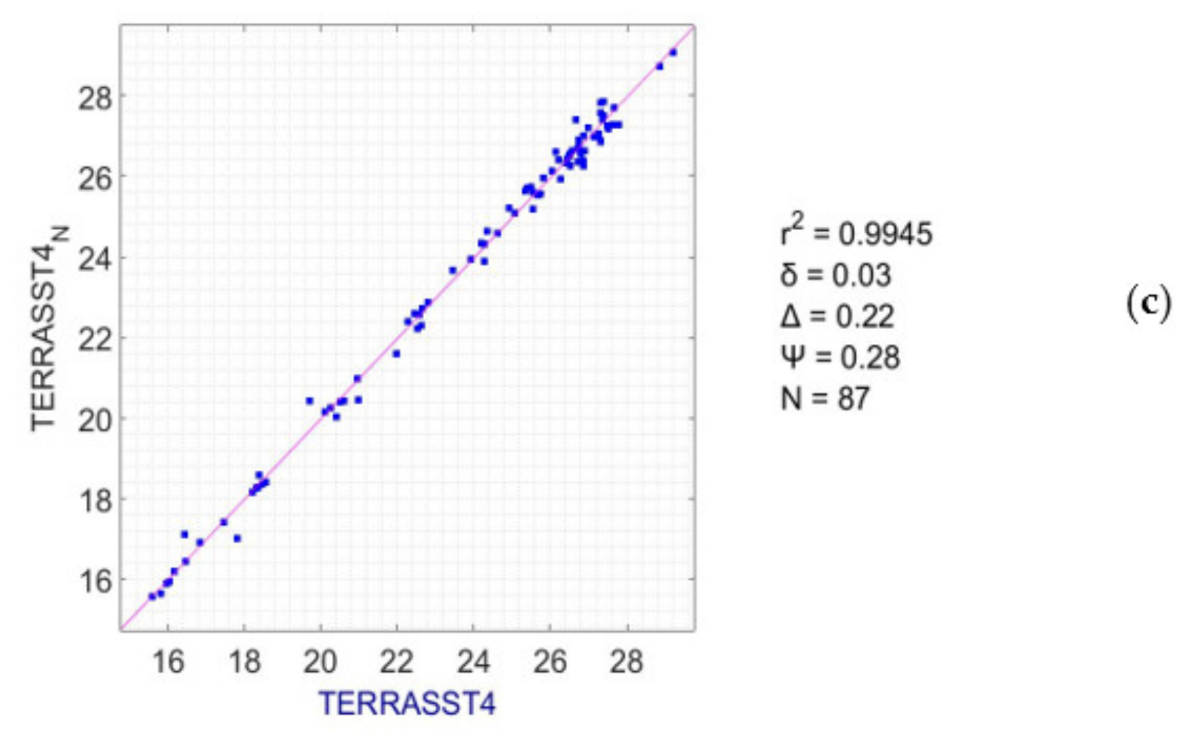Concerning the MODIS Terra SST products, the TERRASST4 data showed the same pattern in the statistical tests as the aforementioned MODIS Aqua products (SSTskin-TERRASST4: δ= −0.35, r² = 0.9689) (Table 2). Moreover, for the location of this study, the nighttime TERRASST4 data were recorded closer to dusk than the nighttime AQUASST4 data, which were recorded later in the night. There is a significant cool skin at night—cooler than at dusk—resulting in the TERRASST4 data having a greater negative bias (δ = −0,35) than the AQUASST4 data (δ = −0.08) when compared to in situ SSTskin data. As a reference, MODIS Terra overpasses in our region occurred around 20:00 UTC and MODIS Aqua overpasses were around 00:00 UTC, and the latest sunset of the year was around 17:40 UTC. Both satellite datasets overestimated the SSTskin measurement when compared with the in situ data of our study area. Furthermore, the comparison between the satellite cell that contains the location of the loggers and the northern adjacent cell—further from the shore—showed an overall positive bias (Table 3), meaning that higher temperature values were recorded in the cell closer to the shore. These results are in good agreement with previous studies that compared satellite SST data with in situ collected data [18,21,22,23,24,25,26,27,28,29,30]. With such good matchups between in situ and satellite measurements, these results and statistics also suggest a potential for the use of UBPC in situ temperature measurements in satellite SST validation.

Recently, Brewin et al. [21] compared AVHRR data in a similar way with in situ data of the English Channel off the coast of Plymouth and showed a higher difference in satellite SST retrievals in near-shore waters than in offshore waters. In their study, the differences between satellite and in situ SST data were well-correlated with land surface temperature and solar zenith angle. For their closest to the coastline location the correlation between in situ and satellite SST data was 0.83 (δ = −0.30, RMSE = 1.30), while for an offshore location, the correlation between in situ and satellite SST data was 0.97 (δ = −0.01, RMSE = 0.48). Worth mentioning here, as discussed in their study [21], the closest satellite pixel to the coastline was closer than 2 km offshore, and potentially influenced by land-contamination, since land may be included within the satellite pixel. For our study, the correlation coefficient was over 0.967, and δ was between −0.35 and −0.08, while RMSE was between 0.42 and 0.76 for the in situ with RS SST comparisons. In general, the correlation results of this study’s comparisons agreed well with the offshore results of Brewin et al. [21]. This may indicate that the land adjacency effect is low enough to allow these good matchups. However, the bias levels indicate that it is still present, although not to such a high degree as the coastline location for Brewin et al. Even though the study by Brewin et al. [21] was with a different satellite SST product, this comparison indicates that the same principles and difficulties govern all satellite derived coastal SST measurements and their validation, particularly the proximity to land.

Another recent study by Bernardello et al. [30], in the Western Mediterranean, is also worth discussing in more detail. This study compared MODIS-Aqua data with in situ temperature data loggers, and pointed to a strong correspondence between satellite and in situ data in their area of study. For their study location, all five in situ datasets, when compared with MODIS-Aqua SST data, had r > 0.98 and −0.27 < δ < 0.24. Their study used a method of reconstructing the temperature for shallow near-shore environments not applicable for satellite validation but for overall variability investigation, intra-seasonal and interannual variability, and unseasonably extreme events. Their results cannot be directly compared with ours, but could provide a direction for future work and comparisons concerning two different regions of the Mediterranean Sea, showing a wider application of satellite SST data reconstruction as a proxy for near-shore habitats monitoring.

With respect to the above discussion—and in fact to all relevant studies for validating coastal satellite SST measurements—this is indicative of some of the major difficulties of gaining consistent and valid satellite SST data in the coastal zone. In contrast with the open ocean SST satellite conditions, in the coastal zone, many extra problems need to be addressed. Not only the very nature of some SST products make it impossible to be of use in the coastal zone, e.g., data collected from MW (microwave) technology sensors have to be 75 km away from land because of large footprints that can overlap land, in contrast to IR (infrared) technology sensors that need to be at least 1 km from the closest shore [18], but also the characteristics of the coastal zone can result in different land adjacency effects on the satellite SST data. The local characteristics of a certain area must be taken into account, particularly for satellite data validation, and need thorough investigation concerning the local geomorphological characteristics, the prevailing oceanographic and atmospheric conditions, and various other factors. For example, Stobart et al. [27] mentioned that sites with adjacent estuaries are characterized by higher SST in the summer and lower in the winter than in situ temperature data, due to fresh, cold water riverine inputs that float above the denser but warmer seawater. For the location of this study, the conditions were locally specific, with the UBPC lying about 2 km offshore the northern coast of Crete. The northern coast of Crete runs almost horizontally on a west-east axis and is open to the wave action of the Aegean Sea and the prevailing northwest winds that dictate a prevailing west-to-east surface current for the UBPC location. The wider study location is affected by local winterbourne steams that flow only after rainfall; thus, the fresh water input and the transportation of suspended matter are very limited in the satellite cell that the measurements are taken. Furthermore, with the MODIS cell spatial resolution at 1 × 1 km the distance of the study location from the closest shore being approximately 2 km makes it sufficiently distant from the coast not to be directly contaminated by land. However, the possibility of a systematic difference between extrapolated SSTskin from 7 m and the actual SSTskin temperature can be addressed only with the installation of close-to-surface in situ loggers that will record any stratification phenomena especially during precipitation and/or periods when the local streams dissipate fresh water in the coastal zone.

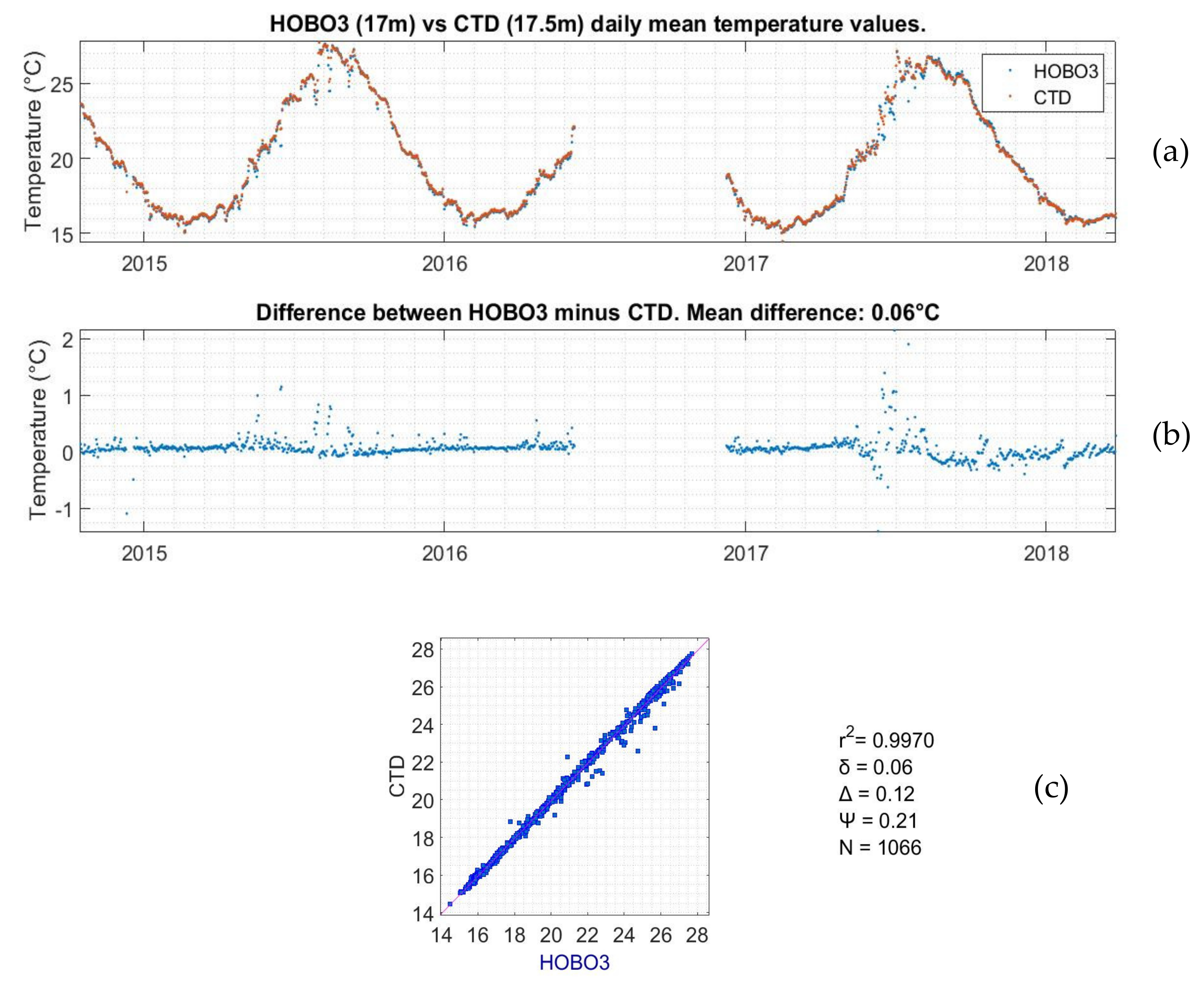
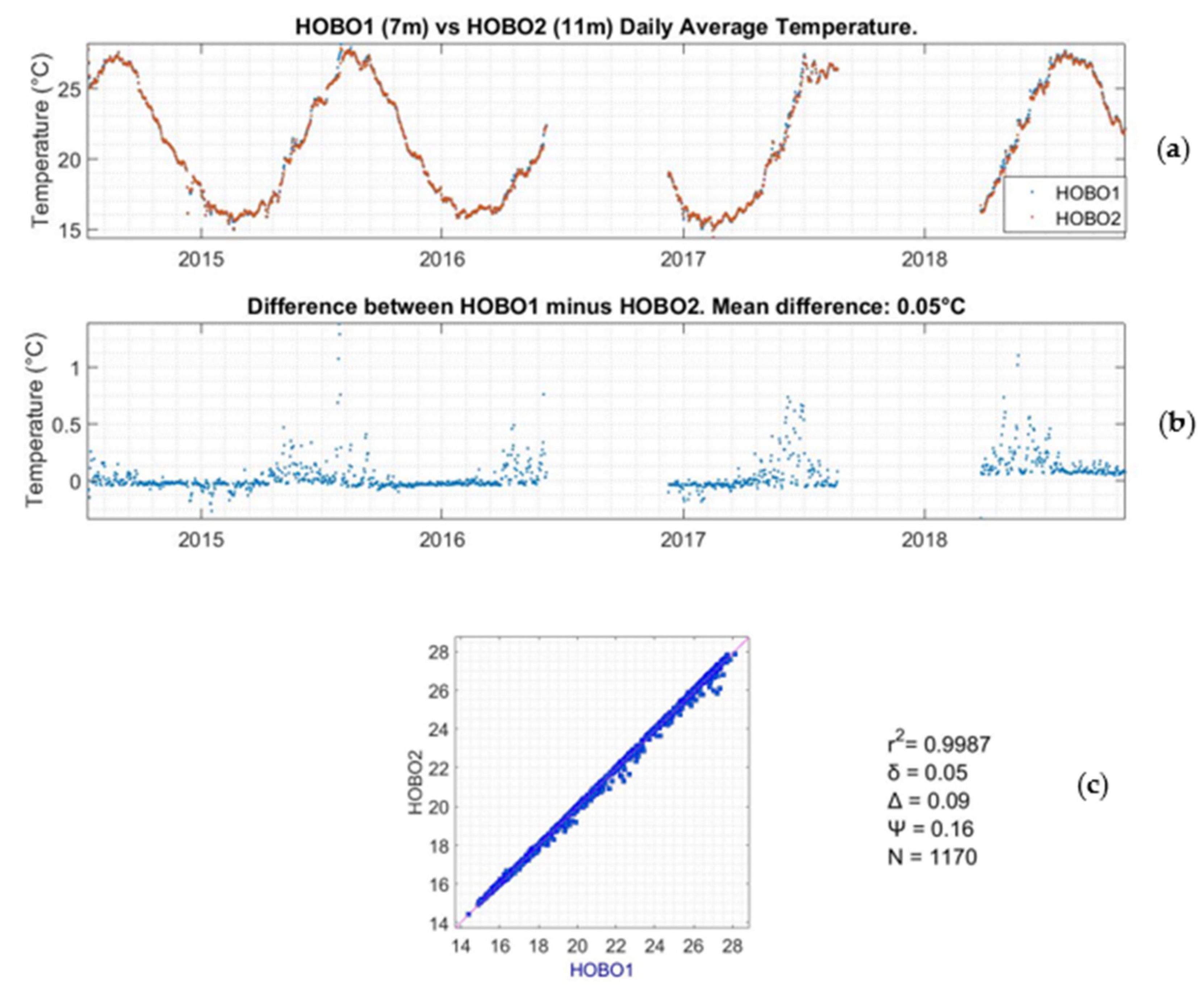
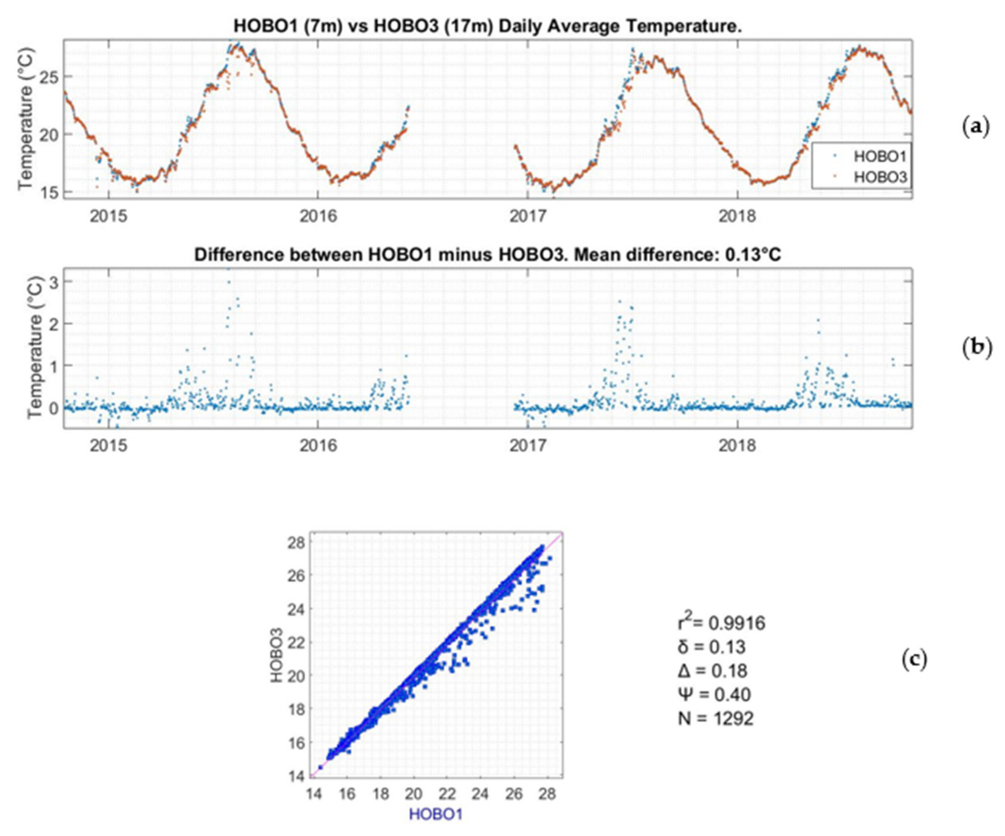
There is also a need to highlight the impact of autonomous in situ sensors, in terms of the applicability of their operating accuracy and uncertainty. Many studies have used autonomous in situ loggers that come with no traceable certificates of calibration, making them prone to add a large amount of uncertainty to satellite measurement validation if they are not at least compared with a sensor that has a traceable calibration certificate and process. Clearly, calibration requirements may raise the financial cost of a study, or exclude datasets with poor accuracy. In this study, for example, the initial deployment of the sensors was to monitor the local environment of the UBPC and only after the comparison between the HOBO3 and the CTD (including a temperature instrument accompanied by a traceable calibration certificate) resulted in very good correlation statistics (r² = 0.9970, δ = 0.06, RMSE = 0.21); thus, it was decided to use the HOBO data series for comparison with the satellite SST data. There is another important factor that should be borne in mind, which had an unknown effect on the results of this study when comparing in situ data with RS SST data. This is the difference of depth in the water column where the measurements took place, i.e. in situ SSTskin data were extrapolated to the surface from the 7 m depth temperature logger and the satellite measurements are of the skin layer taken from above the sea. This has introduced a systematic measurements of temperature bias that is difficult to correct for in the present in situ time series, and thus, promotes the reconfiguration of the UBPC temperature array to include sensors at or close to the surface in order to eliminate the extrapolation necessity as much as possible, and even try to compare RS SST data with daytime in situ SSTskin data.

Nevertheless, most of the studies comparing satellite SST with in situ temperature data still concluded that satellite SST is recommended for environmental/biological studies and can be used as a proxy for temperature in near-shore coastal areas [24,26,28,29]. However, as discussed above and in the introduction, when it comes to the validation of satellite SST measurements, many additional factors have to be taken into consideration. Many of the in situ data are collected from research vessels and are heterogeneous [29] in size, type, and operating footprint, thus creating variable conditions. Additionally, there are many different types of in situ temperature loggers [29] deployed at different depths and, apart from having to account for this depth bias, the main problem with them is the traceability of their calibration and estimating the overall uncertainty budget of their measurements. For example, the HOBO Pro V2 loggers that are widely used -including in this study- have a poor accuracy (±0.2 °C) and resolution (0.02 °C), and their uncertainty budget when operated long-term in the field and when evaluated, may turn out to be unacceptable for evaluating RS SST data. In various studies, the accuracy of the in situ temperature loggers was compared with the accuracy of other instruments with traceable calibration certificates [21,23]. As Castillo and Lima [23] mentioned, even the position of a logger in the water is crucial; when the narrower side of the logger—or its attached shader—faces the sea surface, it is prone to minimal heat exposure.

It is clear that in situ temperature data loggers should provide as accurate a ground truthing factor as possible for the validation of satellite data. Furthermore, it is becoming a prerequisite for any in situ measurements to be used for satellite sensor validation that they should be SI-traceable (SI: International System of Units) with an uncertainty estimate for each measurement. This increasing trend is demanded by the space agencies and follows the recommendations of the Committee on Earth Observation Satellites (CEOS) [44], the Quality Assurance Framework for Earth Observation (QA4EO) guidelines [45], and the European Space Agency (ESA) Fiducial Reference Measurements initiative [46], in particular the project for Fiducial Reference Measurements for Satellite derived Surface Temperature (FRM4STS) [47].

The above suggests further follow-on work concerning our study area and the UBPC, and an attempt will be made to calibrate all the in situ temperature sensors according to FRM principles and to evaluate the additional uncertainty related to using/modeling measurements at a certain depth for the comparison of satellite measurements of the surface. Now that this study has shown the UBPC’s in situ temperature measurement potential for satellite SST validation, this further effort may help to make them more relevant to the space agencies for operational satellite validation. Furthermore, additional in situ temperature loggers are going to be installed, with some as close to the sea surface as possible to help account for the depth of measurement related biases in the in situ time series, something that could also be assisted by comparing our in situ data with an Infrared radiometer that measures the SSTskin-like Infrared Sea-surface temperature Autonomous Radiometer (ISAR) or Marine-Atmospheric Emitted Radiance Interferometer (M-AERI). For these near-surface sensors, following the recommendations of Castillo and Lima [23], the installation will be with their long surface vertical to the sea surface in order to be less affected/biased due to direct solar radiation heating. This will also provide the most accurate method for investigating any stratification phenomena in the study area, since it will as much as possible prevent direct solar radiation heating—which, when using unshaded loggers, can result in areas with transparent clear waters, with erroneously high underwater temperature measurements, according to Bahr et al. [48] and Brewin et al. [49]. A land-based meteorological station is also going to be installed in the vicinity of the study area, so that it will be possible to investigate and quantify any correlations between atmospheric conditions and satellite SST measurement anomalies, following the methods of Brewin et al. [21]. Finally, as there are also biases between different satellite missions, each with their own uncertainties [18,22], following the UBPC temperature sensor upgrade, a separate inter-comparison study is planned between various satellite SST products and the UBPC data to give an indication of the different correspondence between satellite sensors and products when compared to the same in situ data.

5. Conclusions

The four-year (2014–2018) in situ data series recorded from the UBPC in the waters off the northern coast of Crete (approximately 2 km away from the shore) was compared with MODIS Aqua and MODIS Terra SST satellite data. Only data that were within ±1 h of the satellite overpasses were used, and a close correlation was found between these nighttime in situ data and RS products—from Aqua and Terra satellite overpasses (e.g., r² > 0.97, δ < -0.35, Δ < 0.51, Ψ < 0.76 both for Aqua and Terra from the cell that contains the UBPC). When comparing RS data from the cell that contains the loggers with the northern adjacent cell, an overall positive bias occurred, meaning that higher temperature values were recorded closer to the shore.

These matchups between in situ and satellite measurements suggest a potential for the use of UBPC in situ temperature measurements in satellite SST validation. The future plans for the UBPC are therefore not only to continue the operation of the autonomous loggers, but also to add more loggers as close to the sea surface as possible to be closer to the surface (skin) temperature of satellite SST measurements. Furthermore, the establishment of a land meteorological station in the vicinity of the study location will provide information about the interaction and effect of atmospheric conditions on the operation of satellite acquired SST data. However, to be of real use in satellite validation, as part of upgrading the UBPC, it is of prime importance that priority is given to the estimation of the uncertainty budget of the in situ temperature loggers and the traceability of all the calibration procedures of the instrumentation being used. This is in line with the requirements of fiducial reference measurements, an ESA initiative that was set to help guide satellite validation for the future [46].

References

1. European Parliament. The Impact of Tourism on Coastal Areas: Regional Development Aspects, Study of Policy Department B: Structural and Cohesion Policies; European Parliament: Brussels, Belgium, 2008. [Google Scholar]
2. Lu, Y.; Yuan, J.; Lu, X.; Su, C.; Zhang, Y.; Wang, C.; Cao, X.; Li, Q.; Su, J.; Ittekkot, V.; et al. Major threats of pollution and climate change to global coastal ecosystems and enhanced management for sustainability. Environ. Pollut. 2018, 239, 670–680. [Google Scholar] [CrossRef] [PubMed] [Green Version]
3. McCaul, M.; Barland, J.; Cleary, J.; Cahalane, C.; McCarthy, T.; Diamond, D. Combining remote temperature sensing with in-situ sensing to track marine/freshwater mixing dynamics. Sensors 2016, 16, 1402. [Google Scholar] [CrossRef] [PubMed] [Green Version]
4. Thomas, A.; Byrne, D.; Weatherbee, R. Coastal sea surface temperature variability from Landsat infrared data. Remote Sens. Environ. 2002, 81, 262–272. [Google Scholar] [CrossRef]
5. Varela, R.; Lima, F.P.; Seabra, R.; Meneghesso, C.; Gómez-Gesteira, M. Coastal warming and wind-driven upwelling: A global analysis. Sci. Total Environ. 2018, 639, 1501–1511. [Google Scholar] [CrossRef]
6. Yamamoto, T.; Nadaoka, K. Analyzing coastal turbidity under complex terrestrial loads characterized by a “stress connectivity matrix” with an atmosphere-watershed-coastal ocean coupled model. Estuar. Coast. Shelf Sci. 2018, 203, 44–58. [Google Scholar] [CrossRef]
7. Tang, D.; Kester, D.R.; Wang, Z.; Lian, J.; Kawamura, H. AVHRR satellite remote sensing and shipboard measurements of the thermal plume from the Daya Bay, nuclear power station, China. Remote Sens. Environ. 2003, 84, 506–515. [Google Scholar] [CrossRef]
8. Ishizu, M.; Miyazawa, Y.; Tsunoda, T.; Guo, X. Development of a biogeochemical and carbon model related to ocean acidification indices with an operational ocean model product in the north western pacific. Sustainability 2019, 11, 2677. [Google Scholar] [CrossRef] [Green Version]
9. Rabalais, N.N.; Turner, R.E.; Díaz, R.J.; Justić, D. Global change and eutrophication of coastal waters. ICES J. Mar. Sci. 2009, 66, 1528–1537. [Google Scholar] [CrossRef]
10. Nilsson, J.A.; Fulton, E.A.; Johnson, C.R.; Haward, M. How to sustain fisheries: Expert knowledge from 34 nations. Water 2019, 11, 213. [Google Scholar] [CrossRef] [Green Version]
11. Bulleri, F.; Chapman, M.G. The introduction of coastal infrastructure as a driver of change in marine environments. J. Appl. Ecol. 2010, 47, 26–35. [Google Scholar] [CrossRef]
12. Vergés, A.; Steinberg, P.D.; Hay, M.E.; Poore, A.G.B.; Campbell, A.H.; Ballesteros, E.; Heck, K.L.; Booth, D.J.; Coleman, M.A.; Feary, D.A.; et al. The tropicalization of temperate marine ecosystems: Climate-mediated changes in herbivory and community phase shifts. Proc. R. Soc. B 2014, 281, 20140846. [Google Scholar] [CrossRef] [PubMed]
13. Harley, C.D.G.; Randall Hughes, A.; Hultgren, K.M.; Miner, B.G.; Sorte, C.J.B.; Thornber, C.S.; Rodriguez, L.F.; Tomanek, L.; Williams, S.L. The impacts of climate change in coastal marine systems: Climate change in coastal marine systems. Ecol. Lett. 2006, 9, 228–241. [Google Scholar] [CrossRef] [PubMed] [Green Version]
14. Halpern, B.S.; Walbridge, S.; Selkoe, K.A.; Kappel, C.V.; Micheli, F.; D’Agrosa, C.; Bruno, J.F.; Casey, K.S.; Ebert, C.; Fox, H.E.; et al. A global map of human impact on marine ecosystems. Science 2008, 319, 948–952. [Google Scholar] [CrossRef] [PubMed] [Green Version]
15. Hansen, J.; Ruedy, R.; Sato, M.; Lo, K. Global surface temperature change. Rev. Geophys. 2010, 48, RG4004. [Google Scholar] [CrossRef] [Green Version]
16. Lima, F.P.; Wethey, D.S. Three decades of high-resolution coastal sea surface temperatures reveal more than warming. Nat. Commun. 2012, 3, 704. [Google Scholar] [CrossRef] [Green Version]
17. Sea Surface Temperature, Essential Climate Variable (ECV) Factsheet, Global Climate Observing System.
18. Smit, A.J.; Roberts, M.; Anderson, R.J.; Dufois, F.; Dudley, S.F.J.; Bornman, T.G.; Olbers, J.; Bolton, J.J. A coastal seawater temperature dataset for biogeographical studies: Large biases between in situ and remotely-sensed data sets around the coast of south Africa. PLoS ONE 2013, 8, e81944. [Google Scholar] [CrossRef] [Green Version]
19. Banks, A.C.; Mélin, F. An assessment of cloud masking schemes for satellite ocean colour data of marine optical extremes. Int. J. Remote Sens. 2015, 36, 797–821. [Google Scholar] [CrossRef] [Green Version]
20. Mélin, F.; Vantrepotte, V. How optically diverse is the coastal ocean? Remote Sens. Environ. 2015, 160, 235–251. [Google Scholar] [CrossRef]
21. Brewin, R.; Smale, D.; Moore, P.; Dall’Olmo, G.; Miller, P.; Taylor, B.; Smyth, T.; Fishwick, J.; Yang, M. Evaluating operational AVHRR sea surface temperature data at the coastline using benthic temperature loggers. Remote Sens. 2018, 10, 925. [Google Scholar] [CrossRef] [Green Version]
22. Thakur, K.K.; Vanderstichel, R.; Barrell, J.; Stryhn, H.; Patanasatienkul, T.; Revie, C.W. Comparison of remotely-sensed sea surface temperature and salinity products with in situ measurements from British Columbia, Canada. Front. Mar. Sci. 2018, 5, 121. [Google Scholar] [CrossRef] [Green Version]
23. Castillo, K.D.; Lima, F.P. Comparison of in situ and satellite-derived (MODIS-Aqua/Terra) methods for assessing temperatures on coral reefs: Subtidal and SSTs on coral reefs. Limnol. Oceanogr. Methods 2010, 8, 107–117. [Google Scholar] [CrossRef]
24. Delgado, A.L.; Jamet, C.; Loisel, H.; Vantrepotte, V.; Perillo, G.M.E.; Piccolo, M.C. Evaluation of the MODIS-Aqua Sea-Surface Temperature product in the inner and mid-shelves of southwest Buenos Aires Province, Argentina. Int. J. Remote Sens. 2014, 35, 306–320. [Google Scholar] [CrossRef]
25. Baldock, J.; Bancroft, K.P.; Williams, M.; Shedrawi, G.; Field, S. Accurately estimating local water temperature from remotely sensed satellite sea surface temperature: A near real-time monitoring tool for marine protected areas. Ocean Coast. Manag. 2014, 96, 73–81. [Google Scholar] [CrossRef]
26. Smale, D.; Wernberg, T. Satellite-derived SST data as a proxy for water temperature in nearshore benthic ecology. Mar. Ecol. Prog. Ser. 2009, 387, 27–37. [Google Scholar] [CrossRef] [Green Version]
27. Stobart, B.; Mayfield, S.; Mundy, C.; Hobday, A.J.; Hartog, J.R. Comparison of in situ and satellite sea surface-temperature data from South Australia and Tasmania: How reliable are satellite data as a proxy for coastal temperatures in temperate southern Australia? Mar. Freshwater Res. 2016, 67, 612–625. [Google Scholar] [CrossRef]
28. Lathlean, J.; Ayre, D.; Minchinton, T. Rocky intertidal temperature variability along the southeast coast of Australia: Comparing data from in situ loggers, satellite-derived SST and terrestrial weather stations. Mar. Ecol. Prog. Ser. 2011, 439, 83–95. [Google Scholar] [CrossRef] [Green Version]
29. Alvera- Azcárate, A.; Troupin, C.; Barth, A.; Beckers, J.-M. Comparison between satellite and in situ sea surface temperature data in the Western Mediterranean Sea. Ocean Dyn. 2011, 61, 767–778. [Google Scholar] [CrossRef]
30. Bernardello, R.; Serrano, E.; Coma, R.; Ribes, M.; Bahamon, N. A comparison of remote-sensing SST and in situ seawater temperature in near-shore habitats in the western Mediterranean Sea. Mar. Ecol. Prog. Ser. 2016, 559, 21–34. [Google Scholar] [CrossRef] [Green Version]
31. Robles-Tamayo, C.; Valdez-Holguín, J.; García-Morales, R.; Figueroa-Preciado, G.; Herrera-Cervantes, H.; López-Martínez, J.; Enríquez-Ocaña, L. Sea surface temperature (SST) variability of the eastern coastal zone of the gulf of California. Remote Sens. 2018, 10, 1434. [Google Scholar] [CrossRef] [Green Version]
32. Cavalli, R. Retrieval of sea surface temperature from MODIS data in coastal waters. Sustainability 2017, 9, 2032. [Google Scholar] [CrossRef] [Green Version]
33. Cavalli, R. Comparison of split window algorithms for retrieving measurements of sea surface temperature from MODIS data in near-land coastal waters. Int. J. Geo-Inf. 2018, 7, 30. [Google Scholar] [CrossRef] [Green Version]
34. Mueller, J.L.; Austin, R.W.; Morel, A.; Fargion, G.S.; McClain, C.R. Ocean Optics Protocols for Satellite Ocean Color Sensor Validation, Revision 4, Volume I: Introduction. Background and Conventions; NASA Technical Memorandum 2003-21621; NASA Goddard Space Flight Center: Greenbelt, MD, USA, 2003; pp. 1–56.
35. Gerovasileiou, V.; Akel, E.K.; Akyol, O.K.; Alongi, G.; Azevedo, F.; Babali, N.; Bakiu, R.; Bariche, M.; Bennoui, A.; Castriota, L.; et al. New mediterranean biodiversity records. Medit. Mar. Sci. 2017, 18, 355–384. [Google Scholar] [CrossRef] [Green Version]
36. Zenetos, A.; Corsini-Foka, M.; Crocetta, F.; Gerovasileiou, V.; Karachle, P.; Simboura, N.; Tsiamis, K.; Pancucci-Papadopoulou, M.-A. Deep cleaning of alien and cryptogenic species records in the Greek Seas (2018 update). Manag. Biol. Invasions 2018, 9, 209–226. [Google Scholar] [CrossRef] [Green Version]
37. Mytilineou, C.; Akel, E.K.; Babali, N.; Balistreri, P.; Bariche, M.; Boyaci, Y.Ö.; Cilenti, L.; Constantinou, C.; Crocetta, F.; Çelik, M.; et al. New mediterranean biodiversity records. Medit. Mar. Sci. 2016, 17, 794–821. [Google Scholar] [CrossRef] [Green Version]
38. SAIV A/S. Operating Manual for STD/CTD Model SD208 with Sound Velocity & Optional Sensors; SAIV A/S: Bergen, Norway, 2009; pp. 1-01–8-04. [Google Scholar]
39. Minnett, P.; Kaiser-Weiss, A. Discussion document: Near-surface oceanic temperature gradients. Group for High Resolution Sea Surface Temperature (GHRSST), Version 12 January 2012. Available online: https://www.ghrsst.org/wp-content/uploads/2016/10/SSTDefinitionsDiscussion.pdf (accessed on 17 March 2020).
40. Donlon, C.J.; Minnett, P.J.; Gentemann, C.; Nightingale, T.J.; Barton, I.J.; Ward, B.; Murray, M.J. Toward improved validation of satellite sea surface skin temperature measurements for climate research. J. Clim. 2002, 15, 353–369. [Google Scholar] [CrossRef] [Green Version]
41. O’Carroll, A.G.; Eyre, J.R.; Saunders, R.W. Three-way error analysis between AATSR, AMSR-E, and in situ sea surface temperature observations. J. Atmos. Ocean. Technol. 2008, 25, 1197–1207. [Google Scholar] [CrossRef] [Green Version]
42. Gentemann, C.L. Three way validation of MODIS and AMSR-E sea surface temperatures. J. Geophys. Res. Oceans 2014, 119, 2583–2598. [Google Scholar] [CrossRef]
43. Xu, F.; Ignatov, A. Error characterization in i Quam SSTs using triple collocations with satellite measurements. Geophys. Res. Lett. 2016, 43, 10–826. [Google Scholar] [CrossRef]
44. ESA, SPPA, Sensor Performance, Products and Algorithms. Available online: https://earth.esa.int/web/sppa/activities/frm (accessed on 8 January 2020).
45. QA4EO, Quality assurance framework for earth observation. Available online: http://qa4eo.org/ (accessed on 8 January 2020).
46. ESA Fiducial Reference Measurements: FRM. Available online: https://earth.esa.int/web/sppa/activities/frm (accessed on 13 January 2020).
47. Fiducial Reference Measurements for Satellite Ocean Colour. Available online: https://frm4soc.org/ (accessed on 8 January 2020).
48. Bahr, K.D.; Jokiel, P.L.; Rodgers, K.S. Influence of solar irradiance on underwater temperature recorded by temperature loggers on coral reefs: Evaluation of underwater temperature loggers. Limnol. Oceanogr. Methods 2016, 14, 338–342. [Google Scholar] [CrossRef]
49. Brewin, R.J.W.; Cyronak, T.; Bresnahan, P.J.; Andersson, A.J.; Richard, J.; Hammond, K.; Billson, O.; de Mora, L.; Jackson, T.; Smale, D.; et al. Comparison of two methods for measuring sea surface temperature when surfing. Oceans 2020, 1, 2. [Google Scholar] [CrossRef] [Green Version]
Figure 1. (a) Map of the Eastern Mediterranean Sea. (b) Location of the underwater biotechnological park of Crete (UBPC) (red arrow), almost 2 km offshore the northern coast of Crete island in Greece.
Remotesensing 12 01140 g001
Figure 2. The temperature installations in the UBPC: (a) The Seafloor Observatory of the UBPC, bottom moored at approximately 19 m depth. The installed conductivity-temperature-density instrument (CTD) instrument, the Acoustic Doppler Profiler (ADP) and the Fluorometer are shown. (b) A deployed HOBO temperature sensor. The maximum length of the sensor is 11.5 cm and maximum diameter 3 cm. (c) A drawing of the installed temperature instruments. The distance between the CTD and the HOBO3 is 10 m.
Remotesensing 12 01140 g002
Figure 3. (a) Data series of the CTD instrument (accompanied by a calibration certificate) compared to the data series of the HOBO3 logger (no calibration certificate). Both sensors are deployed at almost 17 m below the sea surface. Data points are the daily averaged values of each sensor. (b) Difference between the HOBO3 minus the CTD daily averaged data. For the interruption between June 2016 and December 2016, refer to Table A1. (c) Correlation plot and statistics (refer to Section 2.4 for definitions) for the comparison between the HOBO3 and CTD data.
Remotesensing 12 01140 g003
Figure 4. (a) Data series of the HOBO1 logger deployed 7 m below sea surface compared with the HOBO2 logger data that is deployed 11 m below the sea surface. Data points are the daily averaged values of each sensor only from days that both sensors recorded data. (b) Difference between the HOBO1 minus the HOBO2 daily averaged data. (c) Correlation plot for the comparison between the HOBO1 and HOBO2 data (refer to Section 2.4 for definitions).
Remotesensing 12 01140 g004
Figure 5. (a) Data series of the HOBO1 logger deployed 7 m below the sea surface compared with the HOBO3 logger data that is deployed 17 m below the sea surface. Data points are the daily averaged values of each sensor only from days that both sensors recorded data. (b) Difference between the HOBO1 minus the HOBO3 daily averaged data. (c) Correlation plot between the HOBO1 and HOBO3 data (refer to Section 2.4 for definitions).
Remotesensing 12 01140 g005
Figure 6. (a) SSTskin extracted and averaged data within ±1 h of the respective satellite overpass compared with Aqua Moderate Resolution Imaging Spectroradiometer (MODIS) data from the swath’s cell that contains the Seafloor Observatory from the AQUASST4 dataset. (b) Difference between the SSTskin minus the AQUASST4 dataset. (c) Correlation plot between the SSTskin and the AQUASST4 dataset (refer to Section 2.4 for definitions).
Remotesensing 12 01140 g006
Figure 7. (a) SSTskin extracted and averaged data within ±1 h of the respective satellite overpass compared with Terra MODIS data from the cell that contains the Seafloor Observatory from TERRASST4 dataset. (b) Difference between the SSTskin minus the TERRASST4 dataset. (c) Correlation plot between the SSTskin and the TERRASST4 dataset (refer to Section 2.4 for definitions).
Remotesensing 12 01140 g007
Figure 8. (a) AQUASST (in situ logger’s cell) data compared with AQUASST_N (respective northern adjacent cell) data from the same satellite swath. All data have quality flags of 0, 1, and 2. (b) Difference between the AQUASST minus the AQUASST_N dataset. (c) Correlation plot between the AQUASST and the AQUASST_N dataset (refer to Section 2.4 for definitions).
Remotesensing 12 01140 g008
Figure 9. (a) AQUASST4 (in situ logger’s cell) data compared with AQUASST4_N (respective northern adjacent cell) data from the same satellite’s swath. All data have quality flags of 0, 1, and 2. (b) Difference between the AQUASST4 minus the AQUASST4_N dataset. (c) Correlation plot between the AQUASST4 and the AQUASST4_N dataset (refer to Section 2.4 for definitions).
Remotesensing 12 01140 g009
Figure 10. (a) TERRASST (in situ logger’s cell) data compared with TERRASST_N (respective northern adjacent cell) data from the same satellite’s swath. All data have quality flags of 0, 1, and 2. (b) Difference between the TERRASST minus the TERRASST_N dataset. (c) Correlation plot between the TERRASST and the TERRASST_N dataset (refer to Section 2.4 for definitions).
Remotesensing 12 01140 g010
Figure 11. (a) TERRASST4 (in situ logger’s cell) data compared with TERRASST4_N (respective northern adjacent cell) data from the same satellite’s swath. All data have quality flags of 0, 1, and 2. (b) Difference between the TERRASST4 minus the TERRASST4_N dataset. (c) Correlation plot between the TERRASST4 and the TERRASST4_N dataset (refer to Section 2.4 for definitions).
Remotesensing 12 01140 g011aRemotesensing 12 01140 g011b