Variations in Winter Surface Temperature of the Purog Kangri Ice Field, Qinghai–Tibetan Plateau, 2001–2018, Using MODIS Data


1
Shaanxi Key Laboratory of Earth Surface System and Environmental Carrying Capacity, College of Urban and Environmental Sciences, Northwest University, Xi’an 710127, China
2
Institute of Earth Surface System and Hazards, College of Urban and Environmental Sciences, Northwest University, Xi’an 710127, China
3
CAS Center for Excellence in Tibetan Plateau Earth Sciences, Beijing 100101, China
*
Author to whom correspondence should be addressed.
Remote Sens. 2020, 12(7), 1133; https://doi.org/10.3390/rs12071133
Submission received: 11 March 2020
/
Revised: 27 March 2020
/
Accepted: 31 March 2020
/
Published: 2 April 2020
Abstract
:In the context of global warming, the land surface temperature (LST) from remote sensing data is one of the most useful indicators to directly quantify the degree of climate warming in high-altitude mountainous areas where meteorological observations are sparse. Using the daily Moderate Resolution Imaging Spectroradiometer (MODIS) LST product (MOD11A1 V6) after eliminating pixels that might be contaminated by clouds, this paper analyzes temporal and spatial variations in the mean LST on the Purog Kangri ice field, Qinghai–Tibetan Plateau, in winter from 2001 to 2018. There was a large increasing trend in LST (0.116 ± 0.05 °C·a−1) on the Purog Kangri ice field during December, while there was no evident LST rising trend in January and February. In December, both the significantly decreased albedo (−0.002 a−1, based on the MOD10A1 V6 albedo product) on the ice field surface and the significantly increased number of clear days (0.322 d·a−1) may be the main reason for the significant warming trend in the ice field. In addition, although the two highest LST of December were observed in 2017 and 2018, a longer data set is needed to determine whether this is an anomaly or a hint of a warmer phase of the Purog Kangri ice field in December.
1. Introduction
Land surface temperature (LST), which is an essential variable of the terrestrial energy budget, is a key variable of the surface–atmosphere interface that drives mass and energy exchange between the atmosphere and land surface [1,2,3,4,5], thereby playing a critical role in hydrological, meteorological, environmental, and climate change studies [6,7,8,9,10]. Compared with traditional in situ LST observations that are limited to a small area with relatively homogeneous land-cover types, the thermal infrared satellite remote sensing data available since the 1970s can offer surface temperature information with large spatial coverage and a long time series (depending on the revisit cycle of the satellites). These satellite data have become one of the most important data sources for assessing climate change at regional and global scales [11].
Currently, the sensors most commonly used for LST retrieval include Advanced Very High Resolution Radiometer (AVHRR), Moderate Resolution Imaging Spectroradiometer (MODIS), Thematic Mapper (TM), Enhanced Thematic Mapper Plus (ETM+), and Thermal Infrared Sensor (TIRS) [12,13,14,15]. MODIS thermal infrared data have been available since 2000 with ~1 km spatial resolution, and view the entire surface of the Earth every one to two days [16]. Due to its high spatiotemporal resolution, MODIS LST has been widely used to study spatial and temporal variations in regional surface temperature, especially for polar regions and alpine mountainous areas with harsh environments and sparse observation networks. Many studies have been performed to estimate temperature variations on the Antarctic and Greenland ice sheets using MODIS LST, revealing a warming trend and extreme melting events (LST extremes) in recent years [17,18,19,20]. For the Qinghai–Tibetan Plateau, the MODIS LST product has been applied to the lower-altitude regions (<5000 m) with meteorological observation station data in terms of near-surface temperature estimation, delimitation of permafrost extent, and lake surface temperature analysis [21,22,23,24].
The accuracy of the MODIS LST product on snow/ice surfaces has been extensively studied in the Arctic regions, revealing substantial discrepancies among different regions with diverse altitude and climate conditions, as well as different versions of MODIS LST products [25,26,27,28]. However, the ground-based validation of MODIS LST products is comparatively rare in the high-altitude glaciers of the Qinghai-Tibetan Plateau, possibly due to the very sparse meteorological station network and the relatively small area (mostly <1 km2) of mountain glaciers that are generally represented as mixed pixels of MODIS data. Although Zhang et al. [29] validated the errors of MOD11A1 and MYD11A1 for the Xiaodongkemadi Glacier and the Palongzangbo Glacier on the Qinghai–Tibetan Plateau, their results were based on only two mixed pixels (non-glacier parts accounting for 28% and 32%), which may result in spurious accuracy evaluation of MODIS LST products on mountain glaciers. Currently, it is generally believed that the errors in the MODIS LST product on snow or ice surfaces mainly result from failures in determining cloud contamination, especially of thin clouds. Therefore, when the MODIS LST product is applied on snow or ice surfaces, it is essential to eliminate the pixels affected by cloud via statistical methods [30].
Since the 1980s, mountain glaciers on the Qinghai–Tibetan Plateau have generally suffered from a retreating and thinning trend [31,32]. The role of the EDW effect (elevation-dependent warming) in high-altitude mountainous areas [33,34] is still in question owing to the sparse station distribution and to the errors of both remote sensing surface temperature products and climate models. With the global warming in recent decades, rising temperature has led to intensified glacier ablation on the Qinghai–Tibetan Plateau and consequently unstable runoff of downstream rivers, which might jeopardize the livelihood of hundreds of millions of people in the region [35,36,37]. Moreover, the warming of high-altitude areas is directly related to the occurrence of mountain glacial disasters, such as glacier debris flows, glacial lake outburst floods, and glacier avalanches [38,39,40,41]. Therefore, understanding the warming rate of high-altitude glacial areas has a practical significance for water resources management and safety in the downstream area of glaciers [31]. Although Wu et al. [4] retrieved high-precision mountain glacier surface temperatures from Landsat ETM+ data on the Qinghai–Tibetan Plateau, it is difficult to analyze the interannual variations and trends in the LST retrieved from Landsat thermal infrared data because of 16 day revisit time of the satellite.
As the largest glacier on the Qinghai–Tibetan Plateau of China, the Purog Kangri ice field is an ideal area to study the variations in glacier surface temperature using MODIS LST products. An ice core drilled in the Purog Kangri ice field revealed an evident warming since the 20th century [42]; recent data from optical remote sensing satellites show that the Purog Kangri ice field has shrunk by 15.29 km2 (about 3.6%) from 1992 to 2014 [43], and multi-source Digital Elevation Model (DEM) data indicate an increasing thinning rate of the glacier from −0.049 ± 0.200 m·a−1 from 2000 to 2012 [44] to −0.317 ± 0.027m·a−1 from 2012 to 2016 [45]. All these findings reflect the fact that the high-altitude mountainous areas of the Qinghai–Tibetan Plateau are influenced by global warming, but there remains a lack of quantitative knowledge of the specific rate of warming. It is predicted that the warming rate in the Qinghai–Tibetan Plateau will increase until the end of the 21st century, with more pronounced increases in winter than in summer [46]. The rapid wintertime warming could lead to a reduced glacier cold storage and an earlier glacier ablation season [47]. In addition, the glacier LST will stop increasing after reaching 0 °C during the ablation season, which will affect the calculation of the trends of summer glacier LST. Therefore, this paper attempts to analyze the interannual variations in winter LST on the glacier from 2001 to 2018 using MODIS LST products after eliminating cloud-contaminated pixels, in order to understand the trend of winter LST on the Purog Kangri ice field in the 21st century.
2. Study Site
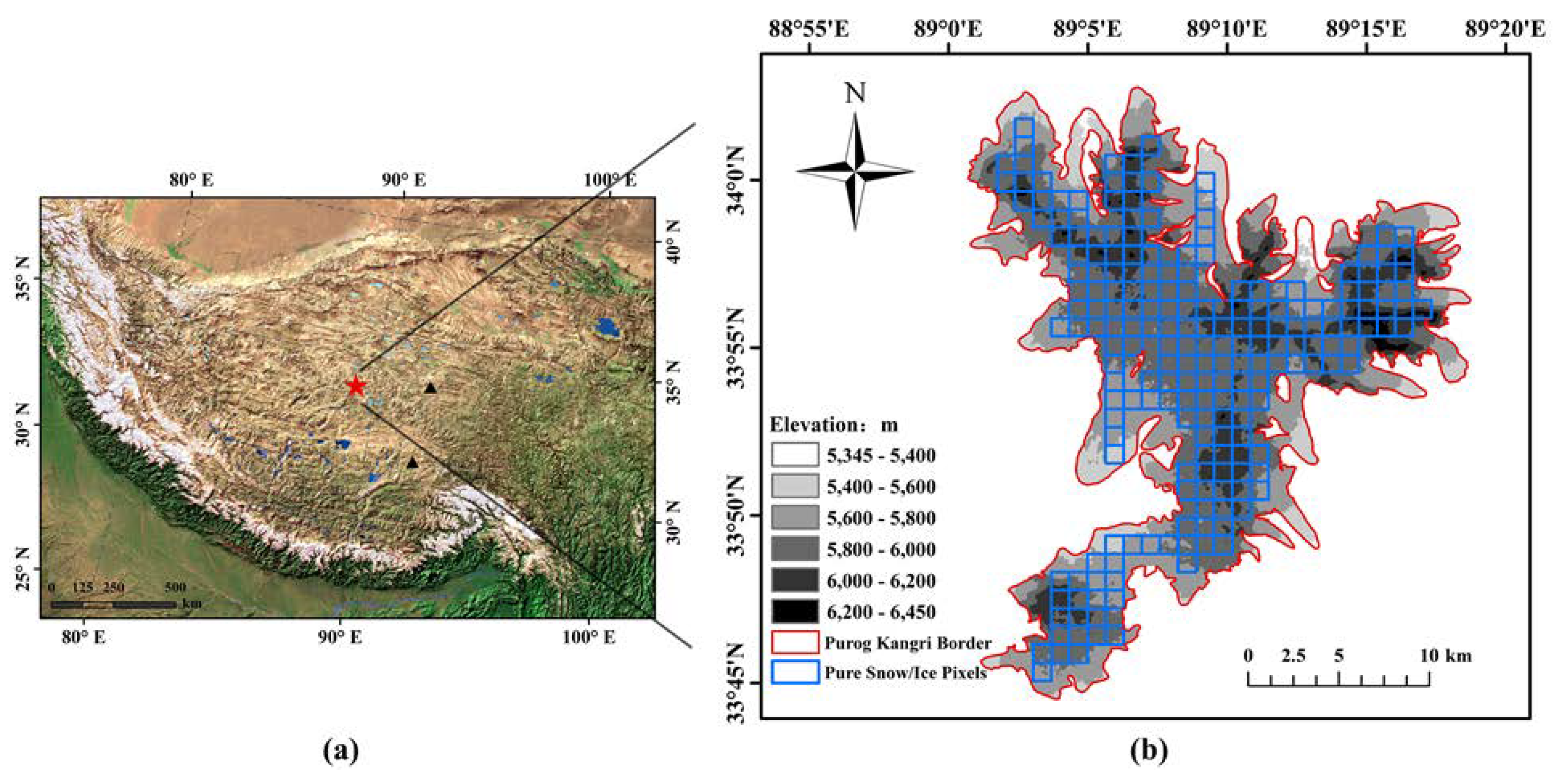
The Purog Kangri ice field (33°44´N–34°03´N, 89°00´E–89°20´E) in the north-central part of the Qinghai–Tibetan Plateau (Figure 1a) covers an area of 422.58 km2 and is the largest ice field in China [48,49]. The ice field is relatively flat over its central part, and is surrounded by more than 50 glacier tongues extending outwards along the mountain valleys, with the longest tongue reaching the foothills (Figure 1). The elevation of the ice field is between 5345 m and 6450 m, and the mean equilibrium-line altitude (ELA is the altitude at which glacier surface accumulation and ablation equal in a year, i.e., the glacier mass balance is equal to 0) during 2001 to 2012 was 5748 ± 37 m [50]. Due to the high altitude and relatively large area, there have only been minor changes in the ice area since the Little Ice Age; in particular the area of the southeastern and western parts is relatively stable, while there is a more obvious shrinkage in the northern part [48].
3. Data and Process
3.1. MODIS LST Products and Processing
The MODIS/Terra and Aqua Land Surface Temperature/Emissivity Daily L3 Global 1 km SIN Grid product is used in this study, which was downloaded from the NASA DAAC (Distributed Active Archive Center) at EROS (Earth Resources Observation and Science) Data Center. Both MODIS/Terra and Aqua pass over the Purog Kangri ice field twice a day, and their overpass times are ~10:30 (MOD11A1_day data)/22:30 (MOD11A1_night data) and ~1:30 (MYD11A1_night data)/13:30 (MYD11A1_day data), respectively. The MOD11A1 and MYD11A1 products are produced with the generalized split-window algorithm that uses MODIS bands 31 and 32 [51] (10.78–11.28 μm and 11.77–12.27 μm, respectively). In 2017, NASA provided a new MODIS LST product (V6), which included the elimination of cloud-contaminated data in MODIS Level 2 and 3, an update of the coefficients of the split-window algorithm, and the adjustment of emissivity values based on ground classification [52]. The detailed information of MODIS LST products and their interactions with other MODIS products can be found in Wan [53,54].
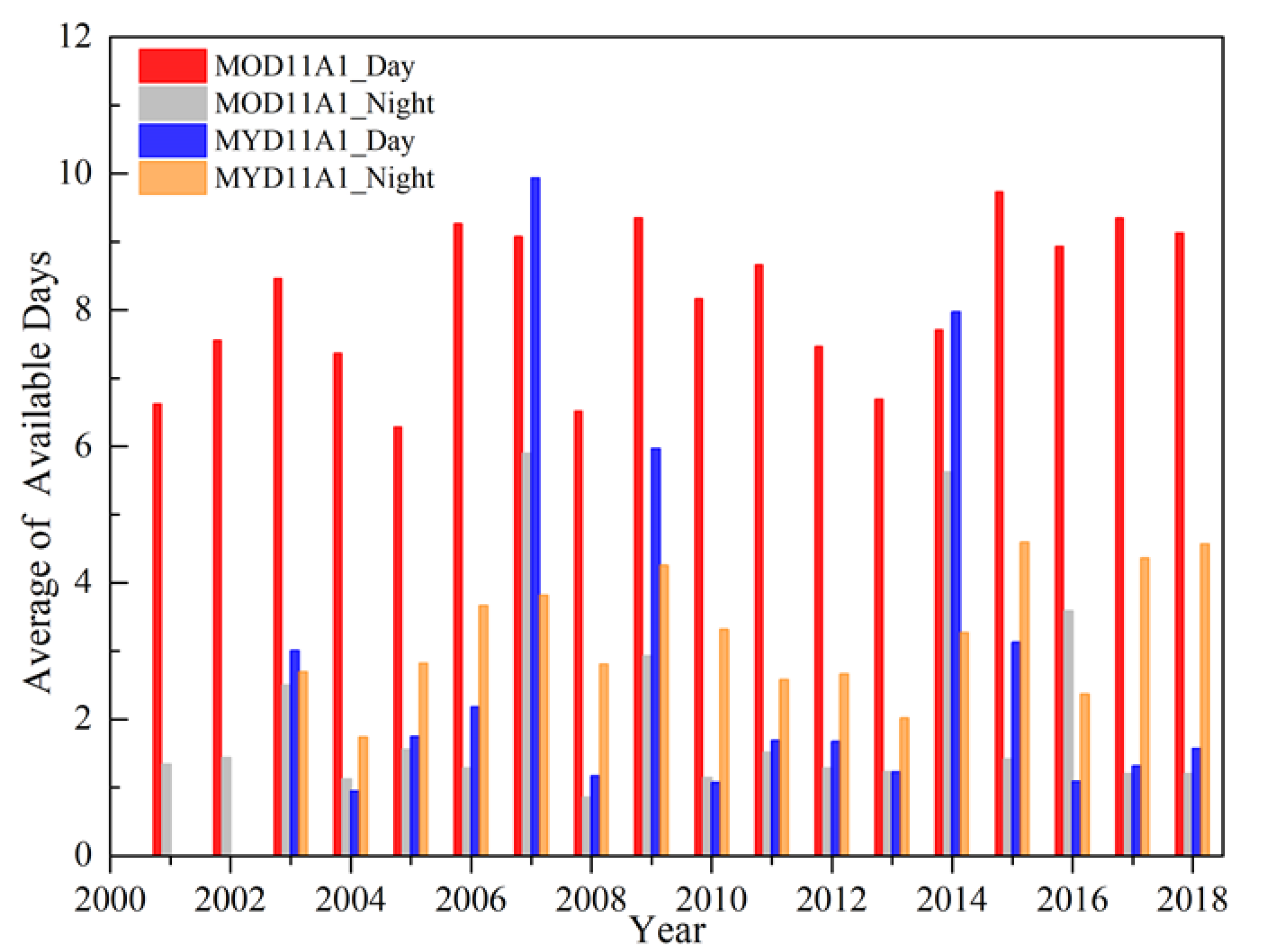
The MOD11A1 and MYD11A1 tile h25v05 provides complete coverage of the Purog Kangri ice field, and data from this tile for the three winter months (December, January, and February) from 2001 to 2018 are used here. The MODIS LST product is reprojected onto a geographic projection using the MODIS Reprojection Tool (MRT) from the original sinusoidal projection, and a total of 212 pixels within the Purog Kangri ice field (according to the Second Glacier Inventory Dataset of China [55]) were used for further study, excluding mixed pixels of glacier and bare rock (Figure 1b). Each grid of MODIS LST product has a quality control (QC) flag ranging from 0 to 3 indicating average errors of <1, 1–2, 2–3, and >3 K. Only pixels which passed quality control at the QC 0/1 level were included for analysis. Cloud contaminated pixels (2) or pixels contaminated for another reason (3) were omitted. The monthly mean available days of four MODIS LST products after quality control (QC) (Figure 2) show that the MOD11A1_day data (red bars) is more appropriate to analyze the variations in LST, while the insufficient availability of the other three data makes it difficult to retrieve a convincing LST trend, the reason for which is also discussed in Section 5.2.
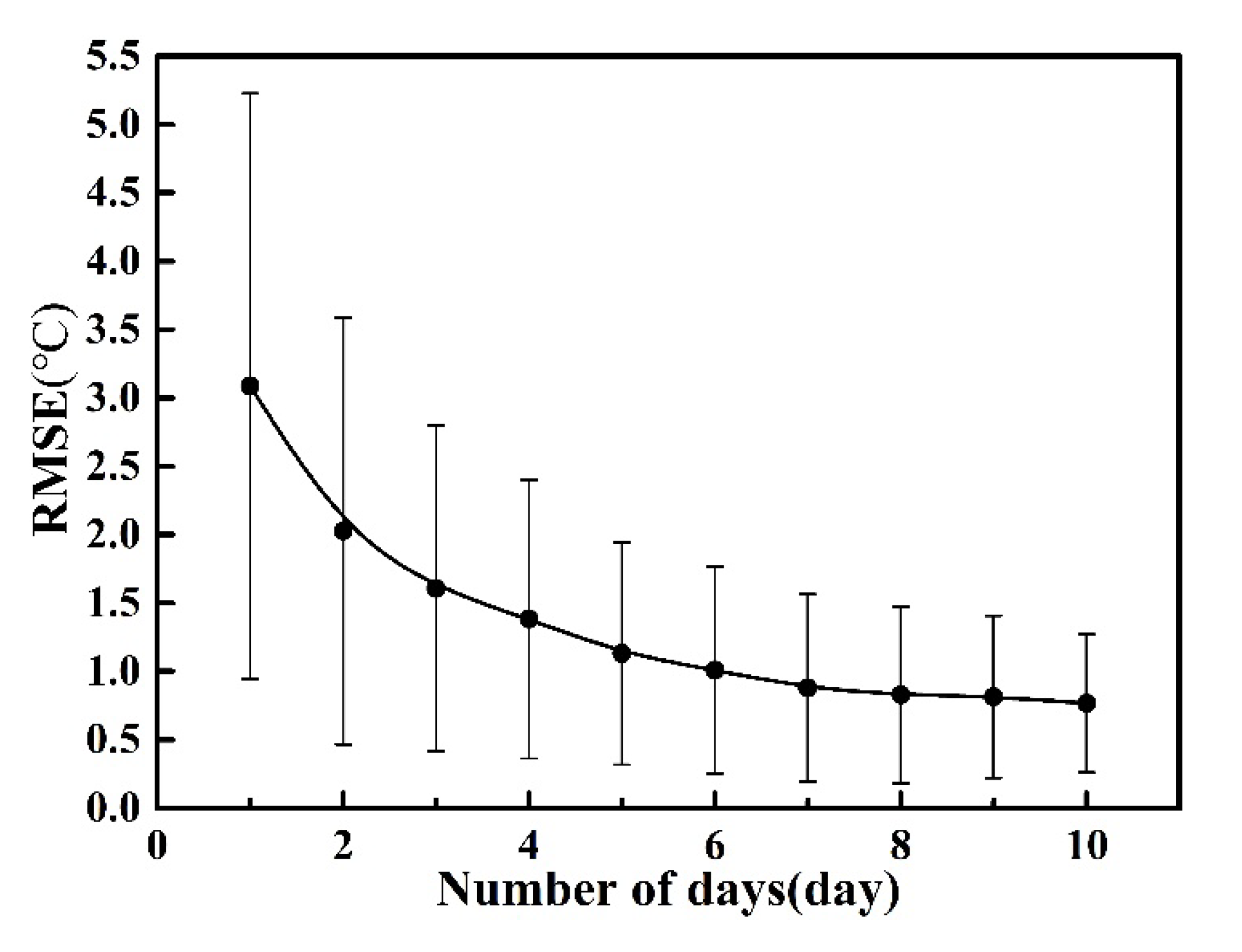
The cloud identification algorithm for the MOD11A1_day products still misses some pixels that are affected by cloud contamination, which is primarily related to thin clouds, cloud shadow contamination, or large view angles [56]. To further improve the data quality and reduce the impact of other sources of uncertainty on the data, following Williamson et al. [30], a 3 × 3 grid cell moving window was used to compare values between each central pixel and its 8 surrounding pixels; the central pixel was excluded if the difference between the central value and the mean (or mean plus standard deviation) of all the surrounding pixels exceeded 5 °C (or 3 °C). After screening for “abnormal” data, the three months have different numbers of valid days with sufficient remaining MODIS pixels. To determine the number of valid days required to adequately represent the monthly mean LST value, the pixel with the greatest number of valid days was selected to calculate the RMSE between the LST averages of randomly selected days and the monthly averages based on the entire dataset. The sample size for each number of days is 10,000. From Figure 3, the RMSE shows a rapid decline when the number of days increases from 1 day to 6 days, and then begins to level off. When the number of days is set to 6 as the threshold for the pixels to be used in this study, the RMSE is around 1. This provides acceptable accuracy for monthly average temperature, while permitting more pixels to be studied. Therefore, in this study, those pixels with at least 6 valid days per month are used to calculate the monthly average LST.
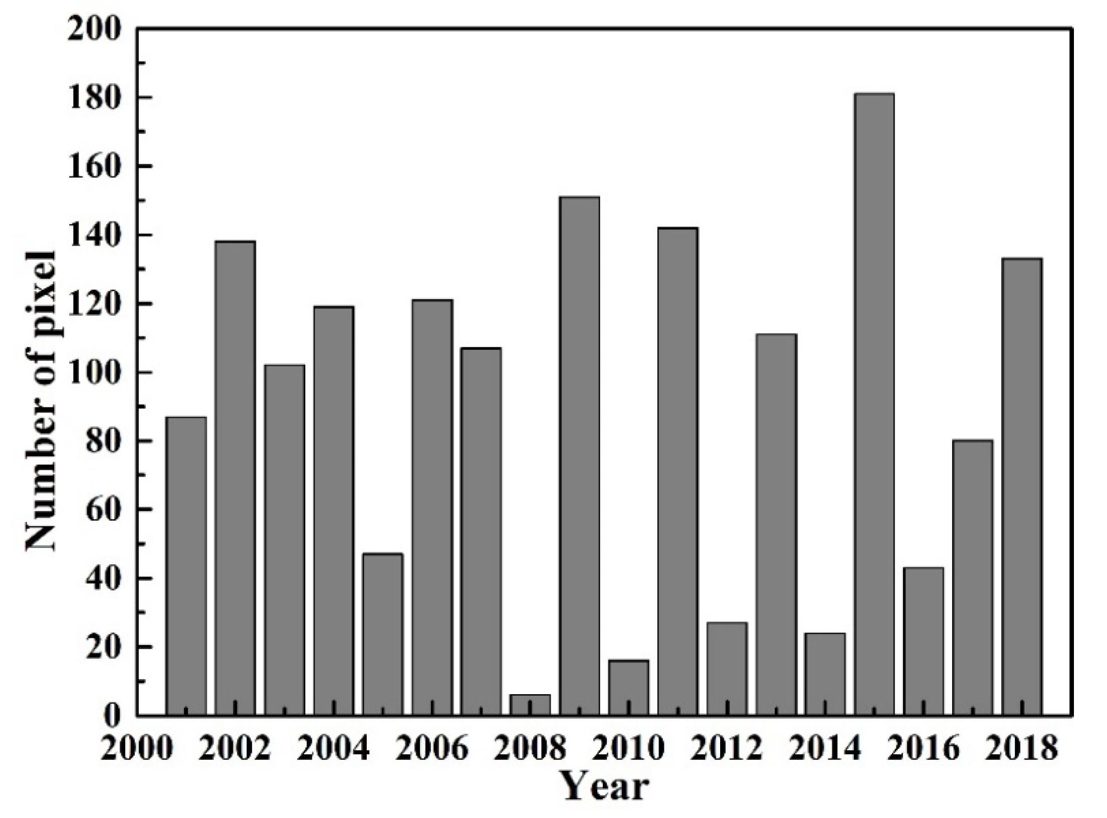
The number of pixels available (more than 6 days of data) from 2001 to 2018 is shown in Figure 4. In some years, excessive cloud cover has reduced the number of pixels, such as 2008 with only 6 pixels available, which may cause large uncertainty in the LST analysis. Therefore, the years of 2005, 2008, 2010, 2012, 2014, and 2016 with too few pixels are excluded in the analysis of LST variations. After data screening, there are 26 pure snow/ice pixels with six days or more of data in December, January, and February together. The analysis of the LST trend in this paper is carried out on those 26 pure ice pixels (shown in Figure 5).
3.2. MODIS Albedo Products
In this study, the MODIS/Terra Snow Cover Daily L3 Global 500m SIN Grid product (MOD10A1 V6) was employed to analyze the trend of albedo; this is available from the NASA DAAC at the National Snow and Ice Data Center (NSIDC). The MOD10A1(V6) contains snow extent, snow albedo, fractional snow cover, and quality assessment data at 500 m resolution and the albedo algorithm within the MOD10A1 algorithm suite was developed by Klein et al. [57]. The MOD10A1 product is generated when the viewing and illumination angles are at the best conditions in a day [58]. The MOD10A1 albedo substantially improved in relative accuracy from V5 to V6 [59]. A description of the MOD10A1(V6) and algorithm can be found in Riggs et al. [60]. The MOD10A1 has been widely validated and is commonly used in the analysis of albedo variation for the surface of snow/ice [61,62]. The MODIS Albedo product is preprocessed with the same method as the MODIS LST data sets.
3.3. Meteorological Data
As there are no long-term meteorological observation data on the Purog Kangri ice field, the monthly mean 2 m air temperatures calculated by averaging the hourly measurements of the two nearest meteorological stations, Nagqu (33°30´N, 92°00´E, altitude 4507 m, 380 km from the ice field) and Tuotuohe (33°12´N, 92°24´E, altitude 4533 m, 310 km from the ice field), was utilized in this study (2001–2018); these data are available from the China Meteorological Science Data Sharing Service Network.
3.4. The High Asia Refined Data
The LST product of High Asia refined (HAR) data is also utilized to be compared with the MODIS LST, which is provided by the Technical University of Berlin [63]. The HAR used a daily reinitialization strategy to prevent drift from observed synoptic conditions during its total simulation period (from October 2000 to October 2014) over the Qinghai–Tibetan Plateau region. The 10-km resolution HAR Surface Skin Temperature (i.e., LST) dataset was dynamically downscaled from the global analysis data using the Weather Research Forecasting model. Although the estimation of the LST trend using HAR data may have some uncertainty, it can still enrich our understanding of temperature variations over the Purog Kangri ice field with no in situ observation.
3.5. Digital Elevation Data
The Advanced Spaceborne Thermal Emission and Reflection Radiometer Global Digital Elevation Model (ASTER GDEM) V2.0 product (2011) with a spatial resolution of 30 m was employed to analyze the relationship between LST and altitude in order to determine if there is an EDW effect in the temperature increase of the Purog Kangri ice field. These data have been widely used for glacier height extraction and topographic analysis in High Mountain Asia [64].
4. Results
4.1. Spatial Pattern in LST Trends of the Purog Kangri Ice Field
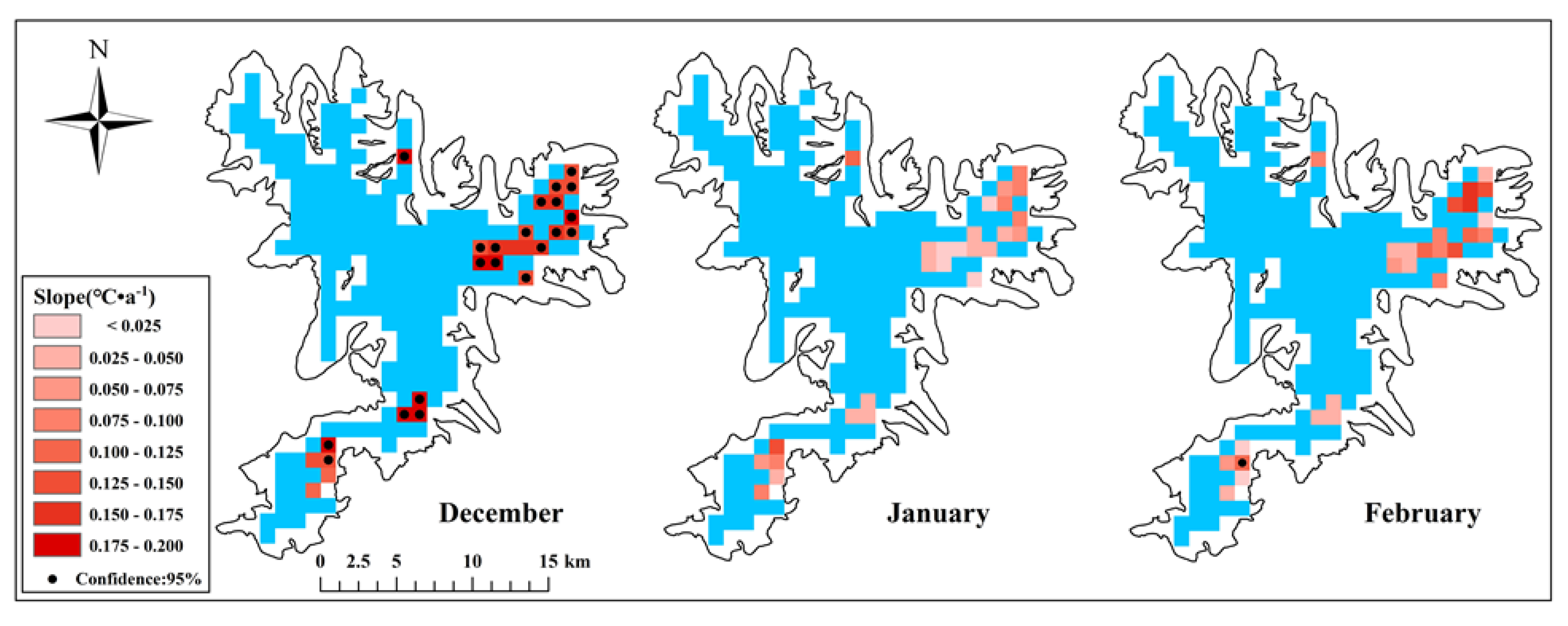
The trend in the wintertime monthly LST during clear daytime over the Purog Kangri ice field is shown in Figure 5, and the nonparametric Mann–Kendall test was used to estimate the significance of the LST trend. December showed the highest rate of warming, with 26 pixels of the ice field having an increasing LST trend of over 0.1 °C·a−1 (22 pixels are significant, p < 0.05). In comparison, although LSTs in January showed increasing trends, they were less than 0.05 °C·a−1 and were not statistically significant (p > 0.05). In February, the increasing trends in LST of most pixels ranged between 0.05 °C·a−1and 0.07 °C·a−1, with only one pixel showing a statistically significant increase (p < 0.05).
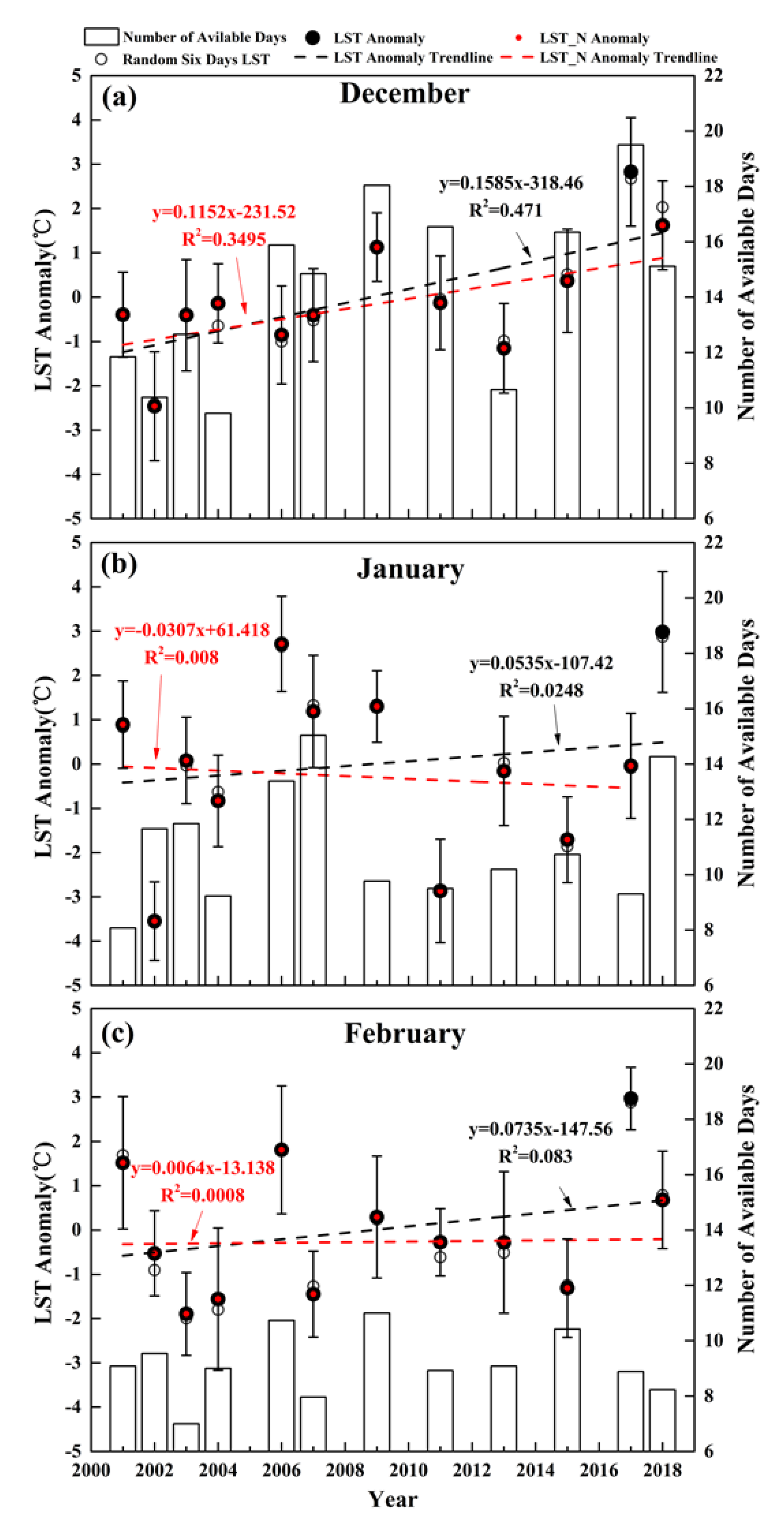
4.2. Variations in the Regional Mean LST of the Purog Kangri Ice Field
The regional mean of all the selected December LST pixels in the Purog Kangri ice field showed an increasing trend of 0.1585 ± 0.053 °C·a−1 (black dashed line in Figure 6a) from 2001 to 2018, with the maximum December LST occurring in 2017, 2.83 °C higher than the 2001–2018 annual average. To avoid the influence of this LST extreme heat on the LST trend, December 2017 was excluded from the trend calculation, and the resultant LST trend still reached 0.1152 ± 0.052 °C·a−1 (red dashed line in Figure 6a), showing a relatively robust trend. In comparison, the LST trend in January was smaller (0.0535 ± 0.106 °C·a−1) and was not statistically significant (black dashed line in Figure 6b). When the year with the maximum January LST (i.e., 2018) was removed, there was even a cooling trend in January (red dashed line in Figure 6b). In February, the overall LST trend of the Purog Kangri ice field was 0.0735 ± 0.077 °C·a−1, which was not statistically significant (black dashed line in Figure 6c), and the temperature trend approached 0 °C·a−1 when the maximum February LST (i.e., 2017) was removed (red dashed line in Figure 6c). Therefore, the warming trends in January and February were sensitive to extremes and were not robust. Of note, although during the period 2001–2018 the LST maximum of all three wintertime months was observed in 2017 or 2018 (Figure 6), a longer data set is needed to determine whether this was an anomaly or just a hint of a warmer phase of Purog Kangri ice field in winter.
Figure 6 shows more available days in December than in January and February, meaning that the monthly mean LSTs of the three winter months are calculated by MODIS LST with different numbers of days, which might affect the consistency of calculated trends among different months. To investigate this issue, the mean LST of 6 random days from December, January, and February for each available pixel was used to represent the corresponding monthly mean LST (gray circles in Figure 6). In fact, there were only small differences (within ±0.2 °C) between the original and the 6-day monthly LST with the exception of some February months that had differences of approximately 0.5 °C, which indicates that using a different number of days (≥6 days) in the calculations of monthly LST has little effect on the calculated trends.
4.3. Influence of Albedo and Number of Clear Days on LST of the Purog Kangri Ice Field
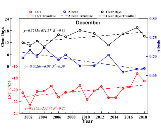
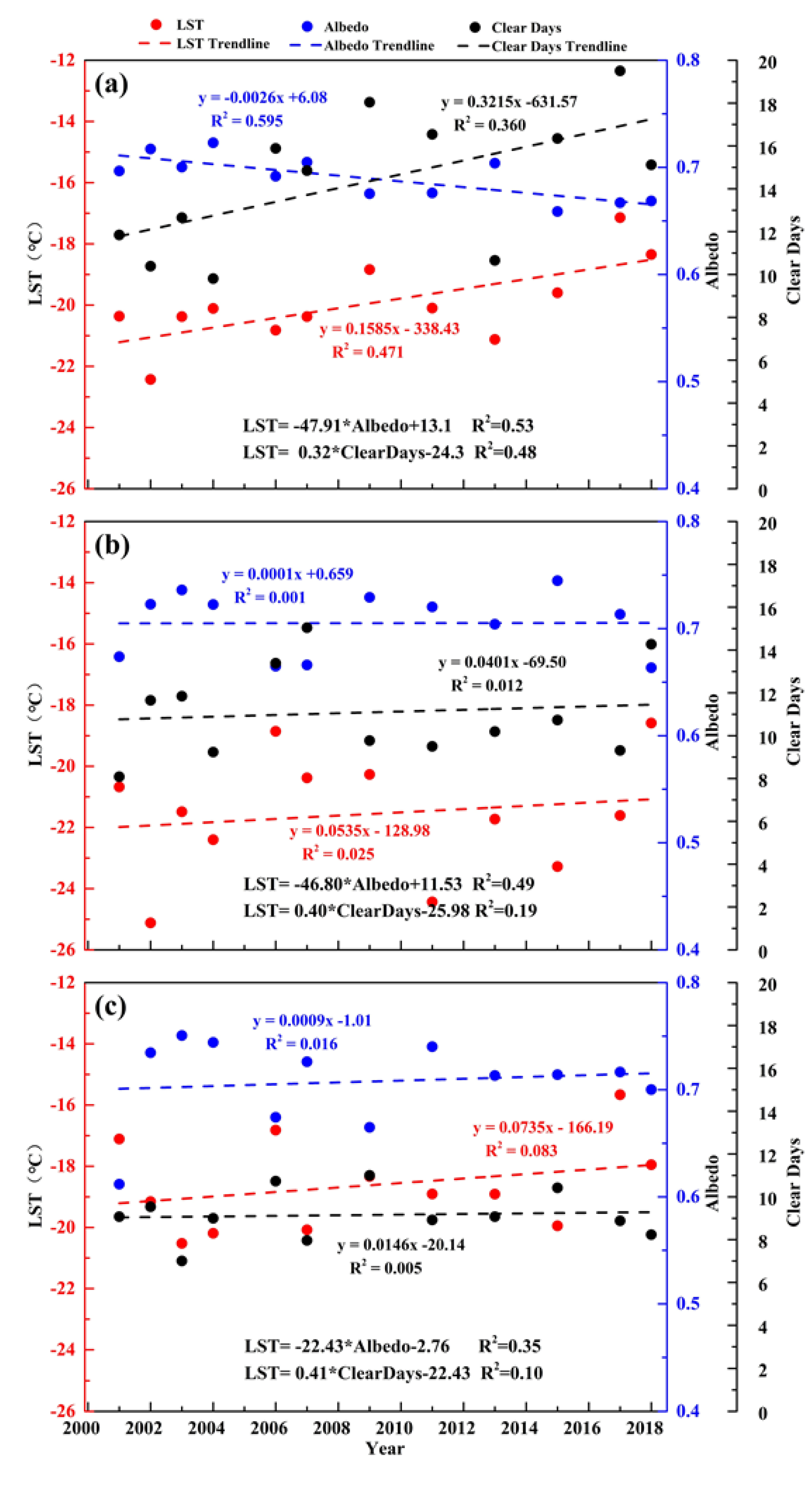
LST is determined partly by surface albedo as it can change the surface energy flux by altering the amount of solar radiation absorbed by the glacier surface [13]. Previous studies (e.g., Nolin et al. [65]) on the Greenland ice sheet indicate that a slight change in ice/snow albedo can trigger substantial fluctuations in the energy flux on the ice surface. From Figure 7, the surface albedo was significantly (p < 0.05) and negatively correlated with LST in all three months of winter during 2001–2018, and the coefficients of determination were 0.53, 0.49, and 0.35 for December, January, and February, respectively. The surface albedo showed a significant decreasing trend in December at a rate of –0.0026 a−1, corresponding with the significant rising trend in LST, whereas for January and February there were no significant trends in either albedo or LST.
In addition, as the main energy source of the ice field, solar radiation (net shortwave radiation) was also controlled by the number of clear days during daytime. From Figure 7, there are positive correlations between the number of clear days and LST for all three months, and the coefficients of determination for December, January, and February were 0.48, 0.19, and 0.10, respectively. Only in December, with a significant LST rising trend, did the number of clear days show a significant increasing trend (about 0.32 d·a−1), whereas in January and February with insignificant LST change trends, the calculated trend of the number of clear days was not statistically significant (p > 0.05).
Therefore, from 2000 to 2018 the significant increasing trend in December LST was evidently affected by the decreasing albedo and the increasing number of clear days, both of which contributed to the increase in solar radiation absorbed by the glacier surface. During the similar time period of our study, the declining trend in winter cloud cover fraction was also consistent with the increasing trend in the number of clear sky days [66,67]. The higher coefficient of determination (0.53) between albedo and LST than that of the number of clear days (0.48) indicated that the LST warming trend in December was more affected by albedo, while the increase of clear days enhanced the effect of the albedo on LST. However, it remains unclear whether the decrease of albedo is the dominant reason for the rising winter LST on glaciers, which needs further field investigation and energy/mass balance simulations.
4.4. Variation of December LST with Elevation on the Purog Kangri Ice Field
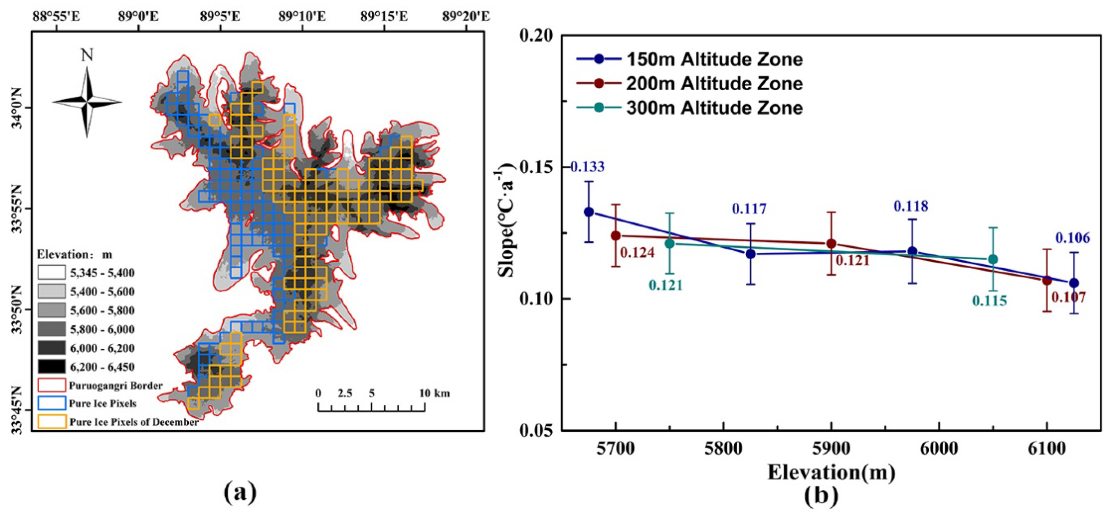
To investigate whether there are variations of LST with elevation in winter for the Purog Kangri ice field, December was taken as an example because it showed a significant warming trend. The altitude range of the Purog Kangri ice field (5600–6200 m) was divided into intervals of 150 m, 200 m, and 300 m so as to separately calculate the LST trend at different altitudes. Note that there are 115 temporally continuous pixels (yellow grid in Figure 8) available in December because they were extracted separately from the MODIS LST product according to the data screening rules (≥6 days). The surface temperature trend was between 0.106 ± 0.012 °C·a−1 and 0.133 ± 0.012 °C·a−1, which decreased slightly with increase in elevation regardless of the interval used in the altitude division.
5. Discussion
5.1. Impact of Data Screening Rules on LST Trends
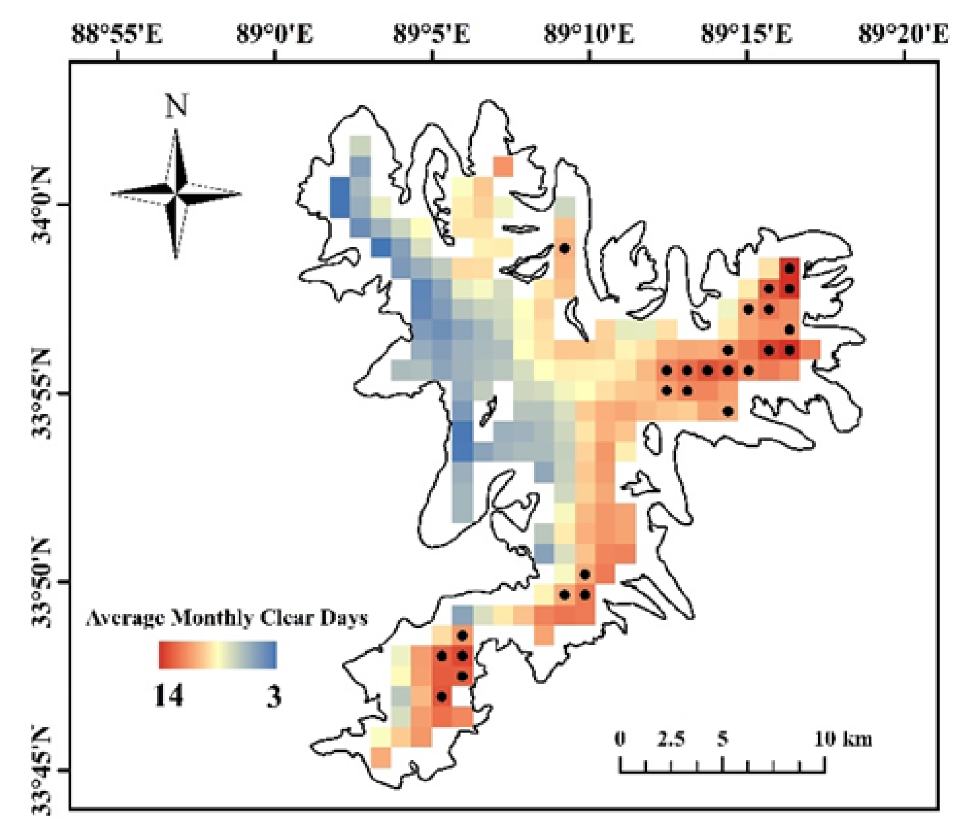
The spatial pattern in the mean number of clear days per winter month (December, January, and February) from 2001 to 2018 shows that the western part of the Purog Kangri ice field is strongly affected by clouds, with only 3–5 clear days available, while the eastern and southern parts are relatively less affected by clouds and thus have 26 pixels selected to study LST variations for all three months (Figure 9).
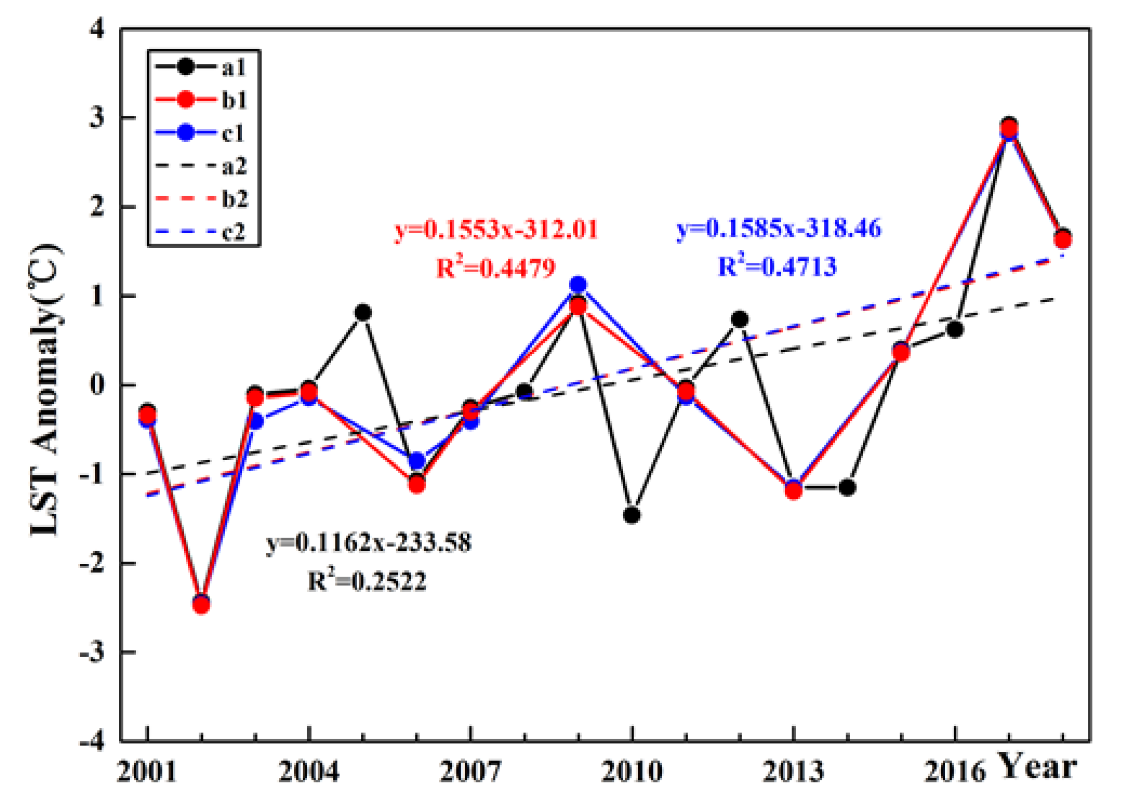
In this study area, the available MODIS data in December was more than in January and February, and 115 pixels were available throughout the period from 2001 to 2018 after data screening. However, the shortage of available MODIS data in January and February meant that six years with too few pixels were removed from trend calculations, which will introduce some errors in the trend analysis when comparing all three winter months. Therefore, the December LST with more available MODIS data was used to estimate the potential influence of data screening with six years missing during the calculation of the LST trend. Comparisons of LST employing three different data sources (using 115 pixels with no years missing, 115 pixels with six years missing, and 26 pixels with six years missing as used in January and February) show almost no difference between the LST variations using 115 pixels and those using 26 pixels (blue and red dots in Figure 10). Therefore, LST using 26 pixels adequately represents the December LST of the corresponding year over the Purog Kangri ice field. However, comparisons show that the December LST trend was overestimated by 0.04 °C·a−1 (the increasing trend was 0.116 ± 0.050 °C·a−1) after excluding six years (black and blue dots in Figure 10). The years with less data availability were often accompanied by an increase of cloud cover. Cloud cover can affect the surface energy balance via radiation forcing, and sometimes increases solar radiation at the surface through multiple reflections between high albedo surface and clouds. Therefore, excluding some years with insufficient data might introduce an error in the LST trend.
5.2. Impact of the Cloud Detection Algorithm of the MODIS LST Product
The cloud detection algorithm in the MODIS LST product cannot identify all types of clouds. Previous research has indicated about 15% undetected cloud contamination in MODIS LST products [68]. Studies on the Arctic Svalbard Archipelago suggest that >40% of the cloud contamination was mistakenly considered as clear sky conditions in the MODIS products, resulting in a large error between the MODIS temperature value and the measured value [27]. The accuracy of the MODIS LST product is mainly limited by the errors from the cloud detection algorithm, and thus it is necessary to employ data screening rules to eliminate potential cloud-contaminated pixels before the trend calculations [25,69].
From Figure 2, it is difficult to retrieve convinced LST trends from the other three MODIS LST products with such insufficient available data, and therefore, only the MOD11A1_day could be used to analyze the LST variations in winter. The availability of MODIS LST products is closely related with cloud cover over the Qinghai–Tibetan Plateau, where there are frequent convective clouds that can blur the glacier LST retrieved from thermal infrared remote sensing. Over the Tibetan plateau, the convective clouds occur primarily at the period of 14:00–20:00, around 02:00, and around 08:00 [70,71], which are basically close to the overpass time of the other three MODIS LST products (i.e., 22:30, 13:30, and 01:30 for MOD11A1 night, MYD11A1_Day, and MYD11A1_night, respectively), while the MOD11A1_Day passes over the ice field (i.e., 10:30) in the period with relatively less convective clouds. Yu et al. [72] found that the mean daily cloud coverage exceeds 45% over the Qinghai–Tibetan Plateau, and the MODIS quality control (QC) data are related to the cloud detection calculation, while Zhang et al. [73] found that high-quality data account for 50%–70% of the total MODIS data. Even with more stringent data quality controls, such as excluding data with errors >1 K, cloud contamination still exists in MODIS LST products. In this paper, the data screening method is only a compromise to remove some of the influence of cloud contamination and will inevitably reduce the amount of available data. Therefore, eliminating the influence of cloud pollution when applying the MODIS LST product in the Qinghai–Tibetan Plateau remains a major challenge.
5.3. Comparisons Between MODIS LST and Station Observations/HAR Dataset
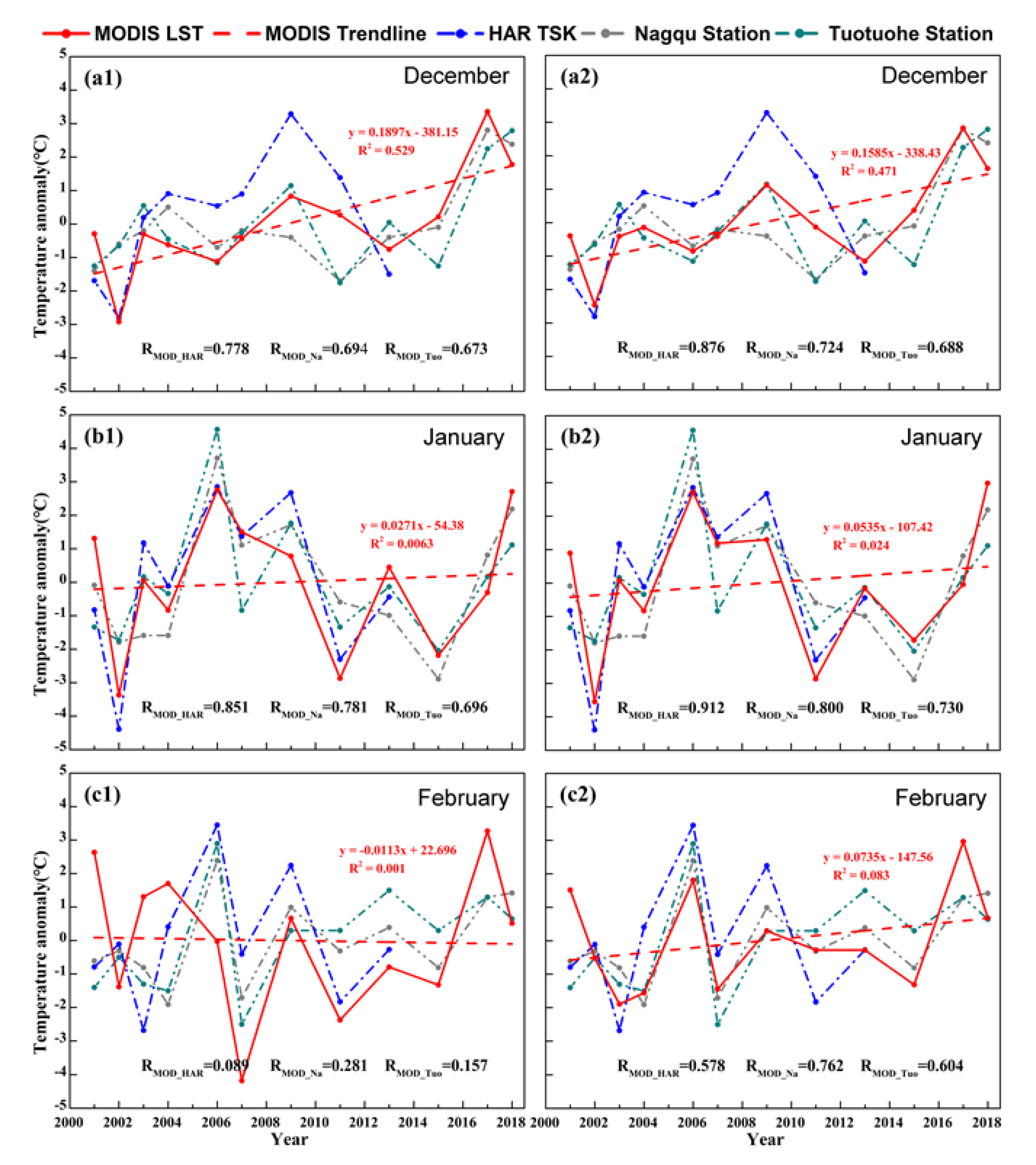
Although the LST trends of the present study were obtained by excluding cloud contamination effects, it is still necessary to check whether they can capture the actual LST variations over the Purog Kangri ice field. As the near-surface temperature is believed to show consistent variations with LST at regional scales [74,75,76], here we compared the 2 m mean air temperature from stations and MODIS LST data with/without data screening, to check if there is a closer relationship between them. In addition, we also added the comparisons between the HAR LST data (10 km) and MODIS LST data on the ice field. Although the estimation of LST trend using HAR data may have some uncertainty, it can still enrich our understanding of temperature variations over the Purog Kangri ice field with no in situ observations. From Figure 11, when the data screening method was utilized, there were obvious increases in correlation coefficients between MODIS LST and the near-surface temperature at both stations and HAR data, especially for February (the month with the most cloud days), which highlights the necessity of a data screening method.
6. Conclusions
Using the MODIS (MOD11A1) daily LST product, this study analyzed the temporal and spatial variations in winter monthly (DJF) LST over the Purog Kangri ice field from 2001 to 2018 by removing MODIS LST pixels that might be contaminated by clouds. The results showed a substantial increasing LST trend (0.116 ± 0.050 °C·a−1) in the ice field during December, while there was no significant LST trend in January and February. The significant reduction in surface albedo of the ice field and the significant increase in the number of clear days may have led to increased solar radiation absorption by the glacier surface, which may be the main reason for the significant warming trend over the ice field in December. This study also showed no evident changes in December LST in different altitude range (5600–6200 m) of the ice field, with only a slight decreasing trend as elevation increases. In addition, the number of pixels available for LST trend calculations was proven to have a limited impact on the trend results, while the elimination of years that were strongly affected by clouds might cause a non-negligible error in the LST trend. Therefore, when using MODIS LST products to analyze LST variations, it is necessary to pay attention to the impact of the eliminated years, and special caution is warranted for results based solely on the years with more clear days. In addition, comparisons between the MODIS LST and near-surface temperature of two nearby stations/HAR LST data showed that it is very necessary to do data screening (6-days cut off and cloud contamination) for MODIS LST products. Given that MODIS LST of only clear days are employed in this study, it is relatively more reliable that December LST was less affected by cloud contamination over the Purog Kangri ice field, while those of other winter months may have some uncertainty. Nevertheless, in the absence of in situ data, the MODIS LST product still offers a valuable data source for us to understand LST variations in high mountain glaciers.
Author Contributions
Conceptualization, N.W.; Data curation, Y.Q. and Y.W.; Formal analysis, Y.W. and A.C.; Funding acquisition, N.W.; Project administration, N.W.; Resources, Y.Q.; Software, A.C.; Supervision, A.C.; Validation, Y.Q. and Y.W.; Visualization, Y.Q.; Writing—original draft, Y.Q.; Writing—review and editing, Y.Q., N.W., and Y.W. All authors have read and agreed to the published version of the manuscript.
Funding
This research was funded by the Strategic Priority Research Program of the Chinese Academy of Sciences (XDA19070302 and XDA20060201), the National Natural Science Foundation of China (41601080), and the Belt and Road Research Program of the Chinese Academy of Sciences (131C11KYSB20160061).
Acknowledgments
The authors would like to acknowledge the National Aeronautics and Space Administration (NASA) for providing MODIS MOD11A1 and MOD10A1 products and ASTER GDEM2 products, the National Snow and Ice Data Center (NSIDC) for offering a platform to download MODIS MOD10A1 products, the Technical University of Berlin for High Asia refined (HAR) data and the China Meteorological Administration for climate data. Special thanks are given to two anonymous reviewers for their fruitful comments and suggestions.
Conflicts of Interest
The authors declare no conflict of interest.
References
- Anderson, M.C.; Norman, J.M.; Kustas, W.P.; Houborg, R.; Starks, P.J.; Agam, N. A thermal-based remote sensing technique for routine mapping of land-surface carbon, water and energy fluxes from field to regional scales. Remote Sens. Environ. 2008, 112, 4227–4241. [Google Scholar] [CrossRef]
- Kalma, J.D.; Mcvicar, T.R.; McCabe, M.F. Estimating land surface evaporation: A review of methods using remotely sensed surface temperature data. Surv. Geophys. 2008, 29, 421–469. [Google Scholar] [CrossRef]
- Li, Z.; Tang, B.; Wu, H.; Ren, H.; Yan, G.; Wan, Z.; Trigo, I.F.; Sobrino, J.A. Satellite-derived land surface temperature: Current status and perspectives. Remote Sens. Environ. 2013, 131, 14–37. [Google Scholar] [CrossRef] [Green Version]
- Wu, Y.; Wang, N.; He, J.; Jiang, X. Estimating mountain glacier surface temperatures from Landsat-ETM + thermal infrared data: A case study of Qiyi glacier, China. Remote Sens. Environ. 2015, 163, 286–295. [Google Scholar] [CrossRef]
- Zhang, R.; Tian, J.; Su, H.; Sun, X.; Chen, S.; Xia, J. Two improvements of an operational two-layer model for terrestrial surface heat flux retrieval. Sensors 2008, 8, 6165–6187. [Google Scholar] [CrossRef] [PubMed]
- Dousset, B.; Gourmelon, F. Satellite multi-sensor data analysis of urban surface temperatures and landcover. ISPRS-J. Photogramm. Remote Sens. 2003, 58, 43–54. [Google Scholar] [CrossRef]
- Hansen, J.R.; Ruedy, R.; Sato, M.; Lo, K. Global surface temperature change. Rev. Geophys. 2010, 48, RG4004. [Google Scholar] [CrossRef] [Green Version]
- Holderness, T.; Barr, S.; Dawson, R. An evaluation of thermal earth observation for characterizing urban heatwave event dynamics using the urban heat island intensity metric. Int. J. Remote Sens. 2013, 34, 864–884. [Google Scholar] [CrossRef] [Green Version]
- Jin, M.; Dickinson, R.E. A generalized algorithm for retrieving cloudy sky skin temperature from satellite thermal infrared radiances. J. Geophys. Res.-Atmos. 2000, 105, 27037. [Google Scholar] [CrossRef]
- Weng, Q. Thermal infrared remote sensing for urban climate and environmental studies: Methods, applications, and trends. ISPRS-J. Photogramm. Remote Sens. 2009, 64, 335–344. [Google Scholar] [CrossRef]
- Kilpatrick, K.A.; Podestá, G.; Walsh, S.; Williams, E.; Halliwell, V.; Szczodrak, M.; Brown, O.B.; Minnett, P.J.; Evans, R. A decade of sea surface temperature from MODIS. Remote Sens. Environ. 2015, 165, 27–41. [Google Scholar] [CrossRef]
- Jimenez, J.C.; Sobrino, J.A.; Skokovic, D.; Mattar, C.; Cristobal, J. Land surface temperature retrieval methods from Landsat-8 thermal infrared sensor data. IEEE Geosci. Remote S. 2014, 11, 1840–1843. [Google Scholar] [CrossRef]
- Nolin, M.; Dickinson, R.E. Land surface skin temperature climatology: Benefitting from the strengths of satellite observations. Environ. Res. Lett. 2010, 5, 044004. [Google Scholar] [CrossRef] [Green Version]
- Roy, D.P.; Wulder, M.A.; Loveland, T.R.; Woodcock, C.E.; Anderson, M.C.; Helder, D.; Irons, J.R.; Johnson, D.M.; Kennedy, R.; Scambos, T.A.; et al. Landsat-8: Science and product vision for terrestrial global change research. Remote Sens. Environ. 2014, 145, 154–172. [Google Scholar] [CrossRef] [Green Version]
- Wang, X. Recent trends in Arctic surface, cloud, and radiation properties from space. Science 2003, 299, 1725–1728. [Google Scholar] [CrossRef] [PubMed]
- Savtchenko, A.; Ouzounov, D.; Ahmad, S.; Acker, J.; Leptoukh, G.; Koziana, J.; Nickless, D. Terra and Aqua MODIS products available from NASA GES DAAC. Adv. Space. Res. 2004, 34, 710–714. [Google Scholar] [CrossRef]
- Hall, D.K.; Williams, R.S.; Luthcke, S.B.; Digirolamo, N.E. Greenland ice sheet surface temperature, melt and mass loss: 2000-06. J. Glaciol. 2008, 54, 81–93. [Google Scholar] [CrossRef] [Green Version]
- Hall, D.K.; Comiso, J.C.; Digirolamo, N.E.; Shuman, C.A.; Box, J.E.; Koenig, L.S. Variability in the surface temperature and melt extent of the Greenland ice sheet from MODIS. Geophys. Res. Lett. 2013, 40, 2114–2120. [Google Scholar] [CrossRef]
- Steig, E.J.; Schneider, D.P.; Rutherford, S.D.; Mann, M.E.; Comiso, J.C.; Shindell, D.T. Warming of the Antarctic ice-sheet surface since the 1957 International Geophysical Year. Nature 2009, 457, 459–462. [Google Scholar] [CrossRef]
- Westermann, S.; Langer, M.; Boike, J. Systematic bias of average winter-time land surface temperatures inferred from MODIS at a site on Svalbard, Norway. Remote Sens. Environ. 2012, 118, 162–167. [Google Scholar] [CrossRef] [Green Version]
- Fu, G.; Shen, Z.; Zhang, X.; Shi, P.; Zhang, Y.; Wu, J. Estimating air temperature of an alpine meadow on the Northern Tibetan Plateau using MODIS land surface temperature. Acta Ecol. Sin. 2011, 31, 8–13. [Google Scholar] [CrossRef]
- Pepin, N.; Deng, H.; Zhang, H.; Zhang, F.; Kang, S.; Yao, T. An examination of temperature trends at high elevations across the Tibetan Plateau: The use of MODIS LST to understand patterns of elevation-dependent warming. J. Geophys. Res.-Atmos. 2019, 124. [Google Scholar] [CrossRef] [Green Version]
- Wan, W.; Li, H.; Xie, H.; Hong, Y.; Long, D.; Zhao, L.; Han, Z.; Cui, Y.; Liu, B.; Wang, C.; et al. A comprehensive data set of lake surface water temperature over the Tibetan Plateau derived from MODIS LST products 2001–2015. Sci. Data 2017, 4, 170095. [Google Scholar] [CrossRef] [PubMed]
- Zou, D.; Zhao, L.; Wu, T.; Wu, X.; Pang, Q.; Qiao, Y.; Wang, Z. Assessing the applicability of MODIS land surface temperature products in continuous permafrost regions in the central Tibetan Plateau. J. Glaciol. Geocryol. 2015, 37, 308–317. [Google Scholar] [CrossRef]
- Adolph, A.C.; Albert, M.R.; Hall, D.K. Near-surface temperature inversion during summer at Summit, Greenland, and its relation to MODIS-derived surface temperatures. Cryosphere 2018, 12, 907–920. [Google Scholar] [CrossRef] [Green Version]
- Koenig, L.S.; Hall, D.K. Comparison of satellite, thermochron and air temperatures at Summit, Greenland, during the winter of 2008/09. J. Glaciol. 2010, 56, 735–741. [Google Scholar] [CrossRef] [Green Version]
- Østby, T.I.; Schuler, T.V.; Westermann, S. Severe cloud contamination of MODIS land surface temperatures over an Arctic ice cap, Svalbard. Remote Sens. Environ. 2014, 142, 95–102. [Google Scholar] [CrossRef]
- Scambos, T.A.; Haran, T.M.; Massom, R. Validation of AVHRR and MODIS ice surface temperature products using in situ radiometers. Ann. Glaciol. 2006, 44, 345–351. [Google Scholar] [CrossRef] [Green Version]
- Zhang, H.; Zhang, F.; Zhang, G.; Ma, Y.; Yang, K.; Ye, M. Daily air temperature estimation on glacier surfaces in the Tibetan Plateau using MODIS LST data. J. Glaciol. 2018, 64, 132–147. [Google Scholar] [CrossRef] [Green Version]
- Williamson, S.N.; Nik, D.S.; Gamon, J.A.; Jarosch, A.H.; Anslow, F.S.; Clarke, G.K.; Rupp, T.S. Spring and summer monthly MODIS LST is inherently biased compared to air temperature in snow covered sub-Arctic mountains. Remote Sens. Environ. 2017, 189, 14–24. [Google Scholar] [CrossRef]
- Liu, S.; Yao, X.; Guo, W.; Xu, L.; Shangguan, D.; Wei, J.; Bao, W.; Wu, L. The contemporary glaciers in China based on the Second Chinese Glacier Inventory. Acta. Geogr. Sin. 2015, 70, 3–16. [Google Scholar] [CrossRef]
- Ye, Q.; Zong, J.; Tian, L.; Cogley, J.G.; Song, C.; Guo, W. Glacier changes on the Tibetan Plateau derived from Landsat imagery: Mid-1970s–2000–13. J. Glaciol. 2017, 63, 273–287. [Google Scholar] [CrossRef] [Green Version]
- Gao, Y.; Chen, F.; Lettenmaier, D.P.; Xu, J.; Xiao, L.; Li, X. Does elevation-dependent warming hold true above 5000 m elevation? Lessons from the Tibetan Plateau. Npj Clim. Atmos. Sci. 2018, 1, 19. [Google Scholar] [CrossRef]
- Pepin, N.; Bradley, R.S.; Diaz, H.F.; Baraer, M.; Caceres, E.B.; Forsythe, N.; Fowler, H.; Greenwood, G.; Hashmi, M.Z.; Liu, X.D.; et al. Elevation-dependent warming in mountain regions of the world. Nat. Clim. Chang. 2015, 5, 424. [Google Scholar] [CrossRef] [Green Version]
- Immerzeel, W.W.; Beek, L.; Bierkens, M. Climate change will affect the Asian water towers. Science 2010, 328, 1382–1385. [Google Scholar] [CrossRef]
- Kehrwald, N.M.; Thompson, L.G.; Yao, T.; Ellen, M.; Schotterer, U.; Alfimov, V.; Beer, J.; Eikenberg, J.; Davis, M.E. Mass loss on Himalayan glacier endangers water resources. Geophys. Res. Lett. 2008, 35, 113–130. [Google Scholar] [CrossRef] [Green Version]
- Yao, T.; Thompson, L.G.; Yang, W.; Yu, W.; Gao, Y.; Guo, X.; Yang, X.; Duan, K.; Zhao, H.; Xu, B.; et al. Different glacier status with atmospheric circulations in Tibetan Plateau and surroundings. Nat. Clim. Chang. 2012, 2, 663–667. [Google Scholar] [CrossRef]
- Chen, D.; Xu, B.; Yao, T.; Guo, Z.; Cui, P.; Chen, F.; Zhang, R.; Zhang, X.; Zhang, L.; Fan, J.; et al. Assessment of past, present and future environmental changes on the Tibetan Plateau. Chin. Sci. Bull. 2015, 60, 3025–3035. [Google Scholar] [CrossRef]
- Kääb, A.; Leinss, S.; Gilbert, A.; Bühler, Y.; Gascoin, S.; Evans, S.G.; Bartelt, P.; Berthier, E.; Brun, F.; Chao, W.; et al. Massive collapse of two glaciers in western Tibet in 2016 after surge-like instability. Nat. Geosci. 2018, 11, 1. [Google Scholar] [CrossRef] [Green Version]
- Liu, X.; Chen, B. Climatic warming in the Tibetan Plateau during recent decades. Int. J. Climatol. 2015, 20, 1729–1742. [Google Scholar] [CrossRef]
- Lu, X.; Kang, S.; Li, Z.; Theakstone, W. Altitude effects of climatic variation on Tibetan Plateau and its Vicinities. J. Earth Sci. China 2010, 21, 189–198. [Google Scholar] [CrossRef]
- Thompson, L.G.; Yao, T.; Mary, E.D.; Ellen, M.; Tracy, A.M.; Lin, P.; Vladimir, N.M.; Victor, S.Z. Holocene climate variability archived in the Puruogangri ice cap on the central Tibetan Plateau. Ann. Glaciol. 2006, 43, 61–69. [Google Scholar] [CrossRef] [Green Version]
- La, B.; Ge, S.; La, B.; You, X.; Pu, B.; De, J. Variation and reasons of the coverage of Puruogangri glacier and its surrounding lakes during 1992-2014. Arid Land Geogr. 2016, 39, 770–776. [Google Scholar] [CrossRef]
- Neckel, N.; Braun, A.; Kropáček, J.; Hochschild, V. Recent Mass Balance of the Purogangri Ice Cap, Central Tibetan Plateau, by Means of Differential X-Band SAR Interferometry. Cryosphere 2013, 7, 1623–1633. [Google Scholar] [CrossRef] [Green Version]
- Lin, L.; Jiang, L.; Sun, Y.; Yi, C.; Wang, H.; Hsu, H. Glacier elevation changes (2012–2016) of the Puruogangri ice field on the Tibetan Plateau derived from bi-temporal TanDEM-X InSAR data. Int. J. Remote Sens. 2016, 37, 5687–5707. [Google Scholar] [CrossRef]
- Xu, Y.; Ding, H.; Li, D. Climatic change over Qinghai and Xizang in 21~(st) Century. Plateau Meteor (In Chinese) 2003, 22, 451–457. [Google Scholar] [CrossRef]
- Li, Z.; Shen, Y.; Wang, F.; Li, H.; Dong, Z.; Wang, W.; Wang, L. Response of glacier melting to climate change-take Ürümqi glacier No.1 as an Example. J. Glaciol. Geocryol. 2007, 29, 333–342. [Google Scholar] [CrossRef]
- Pu, J.; Yao, T.; Wang, N.; Ding, L.; Zhang, Q. Puruogangri ice field and its variations since the Little Ice Age of the Northern Tibetan Plateau. J. Glaciol. Geocryol. 2002, 24, 87–92. [Google Scholar] [CrossRef]
- Yi, C.; Li, X.; Qu, J. Quaternary glaciation of Puruogangri—The largest modern ice field in Tibet. Quat. Int. 2002, 97, 111–121. [Google Scholar] [CrossRef]
- Spiess, M.; Maussion, F.; Marco, M.; Scherer, D.; Schneider, C. MODIS derived equilibrium line altitude estimates for Purogangri ice cap, Tibetan Plateau, and their relation to climatic preditic predictors(2001-2012). Geogr. Ann. Ser. A-Phys. Geogr. 2015, 97, 599–614. [Google Scholar] [CrossRef]
- Wan, Z.; Dozier, J. A generalized split-window algorithm for retrieving land-surface temperature from space. IEEE. Trans. Geosci. Remote. 1996, 34, 892–905. [Google Scholar] [CrossRef] [Green Version]
- Wan, Z. New refinements and validation of the collection-6 MODIS land-surface temperature/emissivity product. Remote Sens. Environ. 2014, 140, 36–45. [Google Scholar] [CrossRef]
- Wan, Z. MODIS Land-Surface Temperature Algorithm Theoretical Basis Document (LST ATBD). Version 3.3; 1999. Available online: https://modis.gsfc.nasa.gov/data/atbd/atbd_mod11.pdf (accessed on 31 March 2020).
- Wan, Z. Collection-6 MODIS Land Surface Temperature Products Users’ Guide. 2013. Available online: https://icess.eri.ucsb.edu/modis/LstUsrGuide/MODIS_LST_products_Users_guide_Collection-6.pdf (accessed on 31 March 2020).
- Guo, W.; Liu, S.; Xu, J.; Wu, L.; Shangguan, D.; Yao, X.; Wei, J.; Bao, W.; Yu, P.; Liu, Q.; et al. The second Chinese glacier inventory: Data, methods and results. J. Glaciol. 2015, 61, 357–372. [Google Scholar] [CrossRef] [Green Version]
- Benali, A.; Carvalho, A.C.; Nunes, J.P.; Carvalhais, N.; Santos, A. Estimating air surface temperature in Portugal using MODIS LST data. Remote Sens. Environ. 2012, 124, 108–121. [Google Scholar] [CrossRef]
- Klein, A.G.; Stroeve, J. Development and validation of a snow albedo algorithm for the MODIS instrument. Ann. Glaciol. 2002, 34, 45–52. [Google Scholar] [CrossRef] [Green Version]
- Riggs, G.A.; Hall, D.K.; Román, M.O. Overview of NASA’s MODIS and visible infrared imaging radiometer suite (VIIRS) snow-cover earth system data records. Earth Syst. Sci. Data 2017, 9, 765–777. [Google Scholar] [CrossRef] [Green Version]
- Casey, K.A.; Polashenski, C.M.; Chen, J.; Tedesco, M. Impact of MODIS sensor calibration updates on Greenland ice sheet surface reflectance and albedo trends. Cryosphere 2017, 11, 1781–1795. [Google Scholar] [CrossRef] [Green Version]
- Riggs, G.A.; Hall, D.K.; Román, M.O. MODIS Snow Products Collection 6 User Guide. 2016. Available online: https://modis-snow-ice.gsfc.nasa.gov/uploads/C6_MODIS_Snow_User_Guide.pdf (accessed on 31 March 2020).
- Stroeve, J.C.; Box, J.E.; Haran, T. Evaluation of the MODIS (MOD10A1) daily snow albedo product over the Greenland ice sheet. Remote Sens. Environ. 2006, 105, 155–171. [Google Scholar] [CrossRef]
- Wang, J.; Ye, B.; Cui, Y.; Yang, G.; He, X.; Sun, W. Accuracy assessment of MODIS daily snow albedo product based on scaling transformation. In Proceedings of the 2011 International Conference on Remote Sensing, Environment and Transportation Engineering, RSETE 2011, Nanjing, China, 24–26 June 2011; pp. 2865–2870. [Google Scholar] [CrossRef]
- Maussion, F.; Scherer, D.; Mölg, T.; Collier, E.; Curio, J.; Finkelnburg, R. Precipitation seasonality and variability over the Tibetan Plateau as resolved by the High Asia Reanalysis. J. Clim. 2013, 27, 1910–1927. [Google Scholar] [CrossRef] [Green Version]
- Hayakawa, Y.S.; Oguchi, T.; Lin, Z. Comparison of new and existing global digital elevation models: ASTER G-DEM and SRTM-3. Geophys. Res. Lett. 2008, 35, 17404. [Google Scholar] [CrossRef]
- Nolin, A.W.; Stroeve, J. The changing albedo of the Greenland ice sheet: Implications for climate modeling. Ann. Glaciol. 1997, 25, 51–57. [Google Scholar] [CrossRef] [Green Version]
- Bao, S.; Letu, H.; Zhao, J.; Shang, H.; Lei, Y.; Duan, A.; Chen, B.; Bao, Y.; He, J.; Wang, T.; et al. Spatiotemporal distributions of cloud parameters and their response to meteorological factors over the Tibetan Plateau during 2003–2015 based on MODIS data. Int. J. Climatol. 2019, 39, 532–543. [Google Scholar] [CrossRef] [Green Version]
- Hua, S.; Liu, Y.; Jia, R.; Chang, S.; Wu, C.; Zhu, C.; Zhu, Q.; Shao, T.; Wang, B. Role of clouds in accelerating cold-season warming during 2000–2015 over the Tibetan Plateau. Int. J. Climatol. 2018, 38, 4950–4966. [Google Scholar] [CrossRef]
- Ackerman, S.A.; Holz, R.E.; Frey, R.A.; Eloranta, E.W.; Maddux, B.C.; Mcgill, M. Cloud detection with MODIS. Part II: Validation. J. Geophys. Res.-Oceans. 2010, 25, 1073–1086. [Google Scholar] [CrossRef] [Green Version]
- Williamson, S.N.; Hik, D.S.; Gamon, J.A.; Kavanaugh, J.L.; Koh, S. Evaluating cloud contamination in clear-sky MODIS Terra daytime land surface temperatures using ground-based meteorology station observations. J. Clim. 2013, 26, 1551–1560. [Google Scholar] [CrossRef]
- Gao, Y.; Jiang, S.; Zhang, Y.; Li, J.; Lin, Z.; Wu, X.; Shen, Z.; Yuan, F.; Huang, C.; Li, C. The Climate of the Tibet; Science Press: Beijing, China, 1984. [Google Scholar]
- Ye, D.; Gao, Y. The Qinghai-Tibetan Plateau Meteorology; Science Press: Beijing, China, 1979. [Google Scholar]
- Yu, J.; Zhang, G.; Yao, T.; Xie, H.; Zhang, H.; Ke, C.; Yao, R. Developing daily cloud-free snow composite products from MODIS Terra-Aqua and IMS for the Tibetan Plateau. IEEE Trans. Geosci. Remote Sen. 2016, 54, 2171–2180. [Google Scholar] [CrossRef]
- Zhang, H.; Zhang, F.; Ye, M.; Che, T.; Zhang, G. Estimating daily air temperatures over the Tibetan Plateau by dynamically integrating MODIS LST data. J. Geophys. Res.-Atmos. 2016, 121, 11425–11441. [Google Scholar] [CrossRef] [Green Version]
- Hall, D.K.; Box, J.E.; Casey, K.A.; Hook, S.J.; Shuman, C.A.; Steffen, K. Comparison of satellite-derived and in situ observations of ice and snow surface temperatures over Greenland. Remote Sens. Environ. 2008, 112, 3739–3749. [Google Scholar] [CrossRef] [Green Version]
- Hall, D.K.; Key, J.R.; Casey, K.A.; Riggs, G.A.; Cavalieri, D.J. Sea ice surface temperature product from MODIS. IEEE Trans. Geosci. Remote Sens. 2004, 42, 1076–1087. [Google Scholar] [CrossRef]
- Shuman, C.A.; Hall, D.K.; DiGirolamo, N.E.; Mefford, T.K.; Schnaubelt, M.J. Comparison of near-surface air temperatures and MODIS ice-surface temperatures at Summit, Greenland (2008–13). J. Appl. Meteorol. Climatol. 2014, 53, 2171–2180. [Google Scholar] [CrossRef]
Figure 1.
(a) Location of the Purog Kangri ice field (red star) and two weather stations (black triangles) and (b) extent of the Purog Kangri ice field. Blue grids denote MODIS (Moderate Resolution Imaging Spectroradiometer) LST (land surface temperature) pixels with underlying surface covered purely by snow/ice.

Figure 2.
Monthly average (DJF) of the available days of MOD11A1_Day (red), MOD11A1_Night (grey), MYD11A1_Day (blue), and MYD11A1_Night data (orange) over the Purog Kangri ice field from 2001 to 2018 after quality control.
Figure 2.
Monthly average (DJF) of the available days of MOD11A1_Day (red), MOD11A1_Night (grey), MYD11A1_Day (blue), and MYD11A1_Night data (orange) over the Purog Kangri ice field from 2001 to 2018 after quality control.

Figure 3.
Variations in RMSE (Root Mean Square Error) with the number of valid days and its error bar (±1 standard deviation).
Figure 3.
Variations in RMSE (Root Mean Square Error) with the number of valid days and its error bar (±1 standard deviation).

Figure 4.
Number of pixels with more than 6 days data available from the 2001 to 2018 winter monthly average LST (land surface temperature) of the Purog Kangri ice field.
Figure 4.
Number of pixels with more than 6 days data available from the 2001 to 2018 winter monthly average LST (land surface temperature) of the Purog Kangri ice field.

Figure 5.
Spatial pattern in LST (land surface temperature) trends for selected pixels during three months (December, January, and February) from 2001 to 2018. Stippled areas show statistically significant trends (p < 0.05). Excluded pixels are shown in blue.
Figure 5.
Spatial pattern in LST (land surface temperature) trends for selected pixels during three months (December, January, and February) from 2001 to 2018. Stippled areas show statistically significant trends (p < 0.05). Excluded pixels are shown in blue.

Figure 6.
Variations in LST (land surface temperature) anomalies (dots) and their linear trend (dashed lines) in (a) December, (b) January, and (c) February over the Purog Kangri ice field. The monthly mean LSTs of all available days during the entire study period are shown in black dots, while those excluding the year with the maximum value are shown in red dots. The histogram indicates the number of days used to calculate the monthly average LST for each month, and the mean LST anomalies calculated from 6 randomly selected days in the month are shown by gray circles.

Figure 7.
Comparison of LST (land surface temperature) (red), surface albedo (blue), and the number of clear days (black) in December, January, and February from 2001 to 2018.
Figure 7.
Comparison of LST (land surface temperature) (red), surface albedo (blue), and the number of clear days (black) in December, January, and February from 2001 to 2018.

Figure 8.
Variations in December LST (land surface temperature) with altitude in the Purog Kangri ice field. (a) The yellow grid shows the 115 temporally continuous pixels of the MODIS LST selected in December. (b) LST trend as a function of altitude of the ice field for three intervals: 150 m, 200 m, and 300 m. Error bars are the ± 1 standard error.

Figure 9.
Average number of clear days per winter month (December, January, and February) from 2001 to 2018. The black dots indicate the 26 pixels that were selected to calculate the LST (land surface temperature) trends for all three winter months.
Figure 9.
Average number of clear days per winter month (December, January, and February) from 2001 to 2018. The black dots indicate the 26 pixels that were selected to calculate the LST (land surface temperature) trends for all three winter months.

Figure 10.
Variations in the December LST (land surface temperature) anomalies (dots) and their linear trends (dashed lines) under different conditions. Those using 115 pixels with no missing years are shown in black (a1 and a2), those using 115 pixels with six years missing are shown in red (b1 and b2), and those using 26 pixels (as used in January and February) with six years missing are shown in blue (c1 and c2).

Figure 11.
Comparisons of anomalies in regional mean MODIS LST (land surface temperature) and HAR (High Asia refined) data over the Purog Kangri ice field as well as the near-surface temperature from two nearby stations (Nagqu and Tuotuohe) in three winter months. Left column: the regional MODIS LSTs are obtained from all the available data after quality control, (a1–c1) for December, January and February; right column: the regional mean MODIS LSTs are obtained from the available data after quality control and data screening, (a2–c2) for December, January and February.

© 2020 by the authors. Licensee MDPI, Basel, Switzerland. This article is an open access article distributed under the terms and conditions of the Creative Commons Attribution (CC BY) license (http://creativecommons.org/licenses/by/4.0/).
Share and Cite
MDPI and ACS Style
Qie, Y.; Wang, N.; Wu, Y.; Chen, A. Variations in Winter Surface Temperature of the Purog Kangri Ice Field, Qinghai–Tibetan Plateau, 2001–2018, Using MODIS Data. Remote Sens. 2020, 12, 1133. https://doi.org/10.3390/rs12071133
AMA Style
Qie Y, Wang N, Wu Y, Chen A. Variations in Winter Surface Temperature of the Purog Kangri Ice Field, Qinghai–Tibetan Plateau, 2001–2018, Using MODIS Data. Remote Sensing. 2020; 12(7):1133. https://doi.org/10.3390/rs12071133
Chicago/Turabian StyleQie, Yufan, Ninglian Wang, Yuwei Wu, and An’an Chen. 2020. "Variations in Winter Surface Temperature of the Purog Kangri Ice Field, Qinghai–Tibetan Plateau, 2001–2018, Using MODIS Data" Remote Sensing 12, no. 7: 1133. https://doi.org/10.3390/rs12071133
Note that from the first issue of 2016, this journal uses article numbers instead of page numbers. See further details here.