Single Channel Source Separation with ICA-Based Time-Frequency Decomposition †


1
Institute of Technical Sciences and Aviation, The State School of Higher Education in Chelm, 22-100 Chelm, Poland
2
Faculty of Mechanical Engineering, Rzeszow University of Technology, 35-959 Rzeszow, Poland
3
Faculty of Mechanical Engineering, Lublin University of Technology, 20-618 Lublin, Poland
*
Author to whom correspondence should be addressed.
†
This paper is an extended version of conference paper. Mika, D.; Budzik, G.; Józwik, J. ICA-based single channel source separation with time-frequency decomposition. In Proceedings of the 6th IEEE Workshop Metro Aerospace, Pisa, Italy, 22–24 June 2020.
Sensors 2020, 20(7), 2019; https://doi.org/10.3390/s20072019
Submission received: 4 March 2020
/
Revised: 25 March 2020
/
Accepted: 2 April 2020
/
Published: 3 April 2020
(This article belongs to the Special Issue Selected papers from the 2020 IEEE International Workshop on Metrology for AeroSpace)
Abstract
:This paper relates to the separation of single channel source signals from a single mixed signal by means of independent component analysis (ICA). The proposed idea lies in a time-frequency representation of the mixed signal and the use of ICA on spectral rows corresponding to different time intervals. In our approach, in order to reconstruct true sources, we proposed a novelty idea of grouping statistically independent time-frequency domain (TFD) components of the mixed signal obtained by ICA. The TFD components are grouped by hierarchical clustering and k-mean partitional clustering. The distance between TFD components is measured with the classical Euclidean distance and the distance of Gaussian distribution introduced by as. In addition, the TFD components are grouped by minimizing the negentropy of reconstructed constituent signals. The proposed method was used to separate source signals from single audio mixes of two- and three-component signals. The separation was performed using algorithms written by the authors in Matlab. The quality of obtained separation results was evaluated by perceptual tests. The tests showed that the automated separation requires qualitative information about time-frequency characteristics of constituent signals. The best separation results were obtained with the use of the distance of Gaussian distribution, a distance measure based on the knowledge of the statistical nature of spectra of original constituent signals of the mixed signal.
1. Introduction
Blind signal separation (BSS) is one of the areas of blind signal processing (BSP), a rapidly developing and very promising field of signal processing. The term “blind” refers to the fact that BPS methods make it possible to separate source signal from mixed signals without the aid of any information or training data. These methods have numerous applications in many research fields, including medical imaging and engineering [1,2,3,4], image processing and speech recognition [5,6] and communication systems [7], as well as astrophysics [8]. In audio engineering, besides speech recognition, BSS can also be used for automatic transcription or speech and musical instrument identification [9].
One of the BSS methods is independent component analysis (ICA) [10], which has gained popularity in a wide range of applications due to its conceptual simplicity and results quality. The ICA technique is a method that uses linear transformation to find statistically independent components from multidimensional mixed data (mixed multichannel signals), assuming that the source signals are statistically independent too. Examples of such multichannel data are audio or vibration signals generated by microphones or vibration sensors recording signals from different measurement points. Standard ICA consists in finding the extreme value of the cost function describing statistical independence, which means that the obtained components will be maximally statistically independent. The efficiency of ICA depends on the cost function selection and the employed optimization strategy [10].
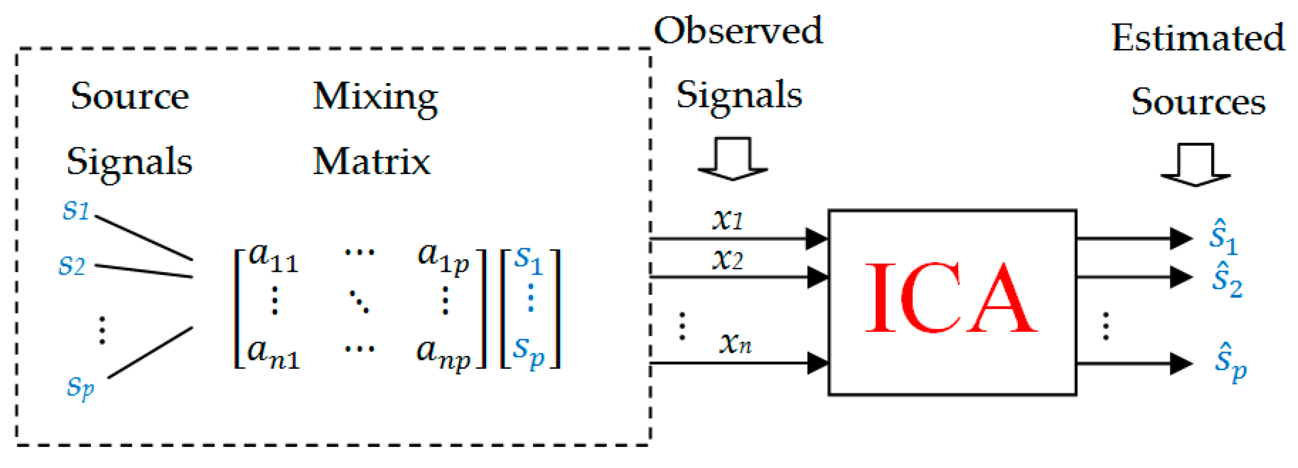
Standard ICA makes use of a multichannel signal, with the number of channels n (the number of microphones or sensors) not being lower than the number of source signals p. ICA consists in calculating statistically independent components (source signals) and a mixing matrix A for only based on n values of observed signals (signals generated by microphones or sensors) . A standard linear ICA model has the form of Equation (1):
where is a vector of observed signals, is a vector of source signals, is an mixing matrix (Figure 1). The separation problem is solved by ICA as Equation (2):
where is an estimation of and matrix is an estimation of the inverse of called filtration matrix. When , the filtration matrix belongs to the general linear group of non-singular matrices .
Usually, the computational complexity of ICA is reduced at the pre-processing stage by so-called whitening the observed signal, which yields a signal , where is the whitening matrix characterized by unitary variance and decorrelation . Assuming that for source signals we obtain Equation (3):
This shows that , or , is an orthogonal matrix (transformation from to takes place via an orthogonal matrix ). Therefore, if , then the matrix is a permutation matrix, and thus a new filtering matrix (after whitening) must also satisfy the orthogonality condition. The solving of the ICA task (when ) is therefore reduced to an optimization on the orthogonal group or the special orthogonal group when compared to the original optimization problem on the group (matrices only satisfying the invertibility condition ). This is connected with a reduction of the degrees of freedom in the problem containing for the matrix on for the matrix .
Standard ICA is based on the assumption that the number of source signals is known and equal to the number of observed signals , i.e., . Still, the ICA estimation can also be performed for a more general case, i.e., when the number of estimated sources p is unknown. In this case, it is possible that . When , i.e., when the number of observed signals is lower than that of source signals, we are dealing with over-complete ICA bases, but when we are dealing with under-complete ICA [11,12]. From a mathematical point of view, such problem can be considered an unconstrained optimization on the Stiefel manifold [13,14,15,16,17].
Many ICA-based methods were used to separate mixed signals [18,19,20,21]. In audio engineering, observed (mixed) signals usually have the form of double channel (stereophonic) or single channel signals. In the case of a single channel signal, which is an “extremely over-complete” ICA model, Equations (1) and (2) cannot be directly employed. In the case of a stereophonic signal, which is known as the problem of under-complete ICA (), differences between channels in intensity and phase of the signals are used for demixing [22,23,24,25]. Wang and Brown [26] introduced a perceptually motivated technique known as the computational auditory scene analysis (CASA) for single channel separation. Nevertheless, it must be emphasized that the effectiveness of such methods is limited and thus some additional a priori information about source signals is required. Most studies in this field are devoted to the extraction (separation) of speech signals [27,28], a commonly used approach is the so-called the W-disjoint orthogonality of signals that assumes their non-overlapping in the time-frequency plane [25,29,30]. Jang and Lee [20] proposed a single channel separation method that use the basis signals obtained by learning the probabilistic properties of sources [31]. Taghia and Doostari [32] used band-wide decomposition of mixed signal components and used ICA for signals mixed in time domain. Davies and James [33] proposed the Single Channel ICA (SCICA) method which is also based on the time domain. In [19] Casey used a single channel separation method that is based on the use of spectrograms of observed signals. In this method, the time-frequency representation of a signal (spectrogram) is treated as a multichannel observed signal and can this be separated by ICA. ICA-obtained statistically independent time-frequency components are then grouped by the Kullback–Liebler measure in order to reconstruct source signals. A similar albeit less complicated approach was adopted by Barry et al. [21]. They separate two signals by using only two spectrogram rows (spectrogram matrix) separated by 330 ms assuming additionally that spectrum of the signals was stationary over this time. A similar approach was taken by Wang and Plumbley [34]. They employed the nonnegative matrix factorisation (NMF) method on the Short Time Fourier Transform (STFT) representation of a single channel observed signal. Their algorithm, however, required the use of an additional training data. In [35], Mijovic employed both wavelet transforms and a combination of empirical mode decomposition (EMD) and ICA for ECG signals decomposition. Methods based on spectral representation of the observed signal are usually known as spectral decomposition-based methods. In [36] Litvin et al. used the bark scale aligned wavelet packet decomposition (BS-WPD) instead of the Fourier transform and at the stage of separation they use the Gaussian mixture model (GMM). In [37], Duan proposed a combination of various single channel separation methods, including some elements of the CASA, spectral decomposition based techniques and model based methods. An excellent overview of single channel source separation methods can be found in [38,39].
The paper is organized as follows. In Section 2 the proposed method of separating single-channel signals is described. There we present subsequent stages of the process and define distance measures used in the method. In addition, the use of linear ICA to solve this type of problem is also explained. In Section 3 the proposed procedure is used to signal source separation of two- and three-component mixed signals, and the quality of obtained separation is discussed in the context of the signal variance used in the analysis. Section 4 presents the results of an auditory test carried out on separated signals. Section 5 discusses the problem of computational complexity of the proposed method and offers a comparative analysis with other simple single-channel separation methods. The results of the analysis are presented in both quantitative and qualitative form. Finally, in Section 6 (Conclusions) the obtained separation results are summarized with respect to the impact of the number of source components, the spectral type of sources, as well as the impact of the signal variance used in the analysis.
2. Model Definition and Procedure
The proposed concept involves the use of ICA for the time-frequency t-f representation (spectrogram) of a single-channel observed signal. The representation of signal in the form of a spectrogram is actually a non-linear transformation (quadratic transformation). In this case, the use of non-linear BSS (non-linear ICA) would be appropriate. It is well known that nonlinear ICA is a difficult problem and it is generally impossible to identify unambiguously true sources [40,41]. However, under certain conditions linear ICA can be used to solve nonlinear BSS. The theoretical conditions for the use of a linear encoder, i.e., cascade PCA and linear ICA to solve a non-linear problem and reconstruct of real independent sources, are presented in [42]. Solutions are asymptotically achieved when the number of sources is high, and the numbers of inputs (mixed signals) and non-linear bases are large relative to the number of sources . In our approach, this condition is satisfied, i.e., , which means that the use of linear ICA is justified in this case.
To this end, the time signal was analysed by the Short Time Fourier Transform (STFT) in compliance with Equation (4):
where is the complex matrix of t-f containing in -rows instantaneous signal spectra ( is the number of STFT time frames). The input data for ICA is a spectrogram (autospectrum) of the signal [43,44]. The rows of the matrix are treated as individual channels in a multichannel signal. By applying the ICA on this multichannel signal, we obtain spectral components of the t-f representation of a single channel signal which are statistically independent. The following relation holds between a and matrix a matrix of statistically independent spectral components as seen in Equation (5):
where is a mixing matrix, is an i-th column of , is an i-th row of , is an i-th t-f component of a mixed one-channel signal.
Throughout this paper, the components are called spectral bases whereas the columns of T describing time variation of are called time bases and denoted by . The matrix , which is the product of the time basis and the spectral basis , is called i-th t-f component. By an appropriate grouping of bases into subgroups generating constituent components of the mixed signal, this mix can be decomposed into components (for comparison, see Equation (1)) using Equation (6):
where are index sets obtained by grouping bases.
In [45,46], the single channel signal decomposition was done by the grouping of time bases and frequency bases .
For practical reason, to reduce computational complexity, it is convenient to only use the bases which “carry” a specified variance of the mixed signal. Assuming that in the analysis we use of signal variance, Equation (5) has the following form in Equation (7):
where the index corresponds to the number of bases “carrying” variance of the mixed signal. The selection of determines the number of bases that are subsequently used in ICA estimation. These bases span a subspace of the primary which is maximally energetic.
The grouping of bases is, in fact, a clustering process, i.e., collecting elements into clusters [47,48]. Clustering results depend on many factors, such as the employed distance measure and clustering algorithm. The distance between base components can be defined in many ways. The selection of a given distance measure type depends on many factors, including the frequency composition of signals, degree of overlapping of signals in time and frequency, the required quality of separation and frequency-related similarity of constituent signals of the mix. In the present experiment, two types of grouping were applied. The first was based on the use of clustering algorithms (hierarchical and k-mean clustering), while the other involved the maximization of negentropy of separated components. ICA-based single channel separation methods primarily use component grouping based on similarity in time or frequency domain. We suggest the use of a time-frequency structure to measure the similarity features in both time and spectral domain. We cluster the (TFD)^i bases using two types of distance between bases, i.e., the classic Euclidean distance and the distance , which we call in this study as the distance of Gaussian distribution. The Euclidean distance is defined as Equation (8):
where denotes the Frobenius norm. The generalized Gaussian distribution is expressed by Equation (9) [49]:
where are the expected value and the standard deviation of a random variable , respectively. The parameter describes the type of a random variable , i.e., its deviation from normal distribution. The parameters and are defined by Equations (10) and (11):
where is the Gamma-Euler function.
By treating a signal spectrogram as a random variable one can describe its distribution in parametric terms, i.e., it is possible to estimate the parameters based on the model in Equation (9). When the source spectrograms are known, we can find the parameter . The distance is defined as the difference between and the parameter characterising the spectrogram of a constituent signal reconstructed after grouping (index was defined in Equation (6)) in the following way in Equation (12):
By minimizing the distance for individual constituent signals one can group bases so that the reconstructed signals are statistically as close as possible to the original signals. The parameter we estimated by a posteriori determination of the maximum of . When observations of the random variable are available the a posteriori distribution of the parameter is given by Equation (13) [10,18]:
where denotes a data likelihood [18] and is an a priori distribution of the parameter. The study [18] offers practical recommendations (solutions) for calculating the distribution.
The other way of grouping bases consists in maximizing negentropy (negative entropy) of reconstructed constituent signals . Statistically independent constituent signals have the maximum negentropy [10,50]. By finding of reconstructed constituent signals with the maximum negentropy, we group the bases in a correct way. The negentropy function was approximated as Equation (14) [10]:
where is the normalized Gaussian random variable () and is a nonlinear function of the random variable usually having the form or . This type of approximation has numerous advantages including conceptual simplicity and rapid calculation rate [10]. As a result, it is very often used as a cost function in algorithms for solving ICA problems [51].
3. Experiment
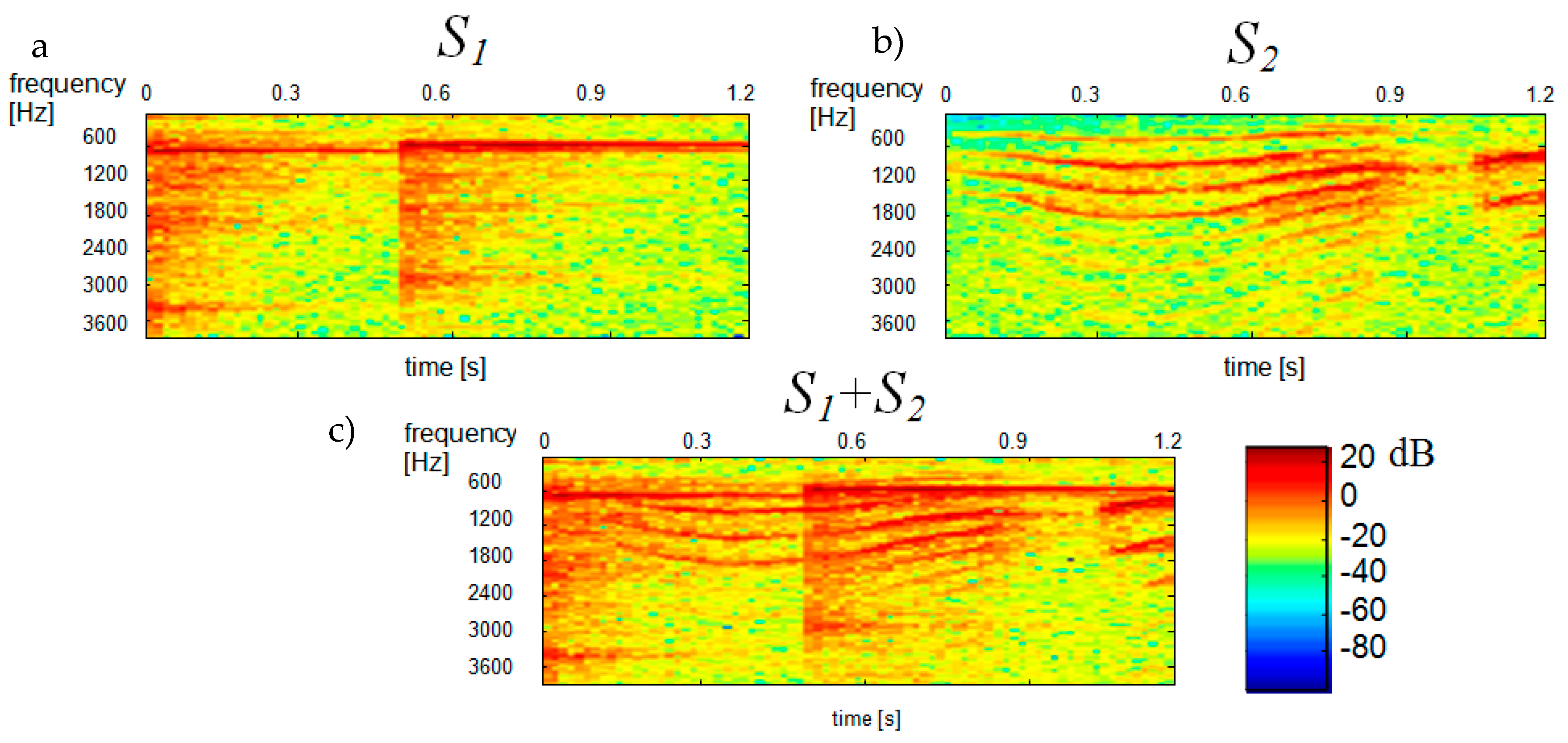
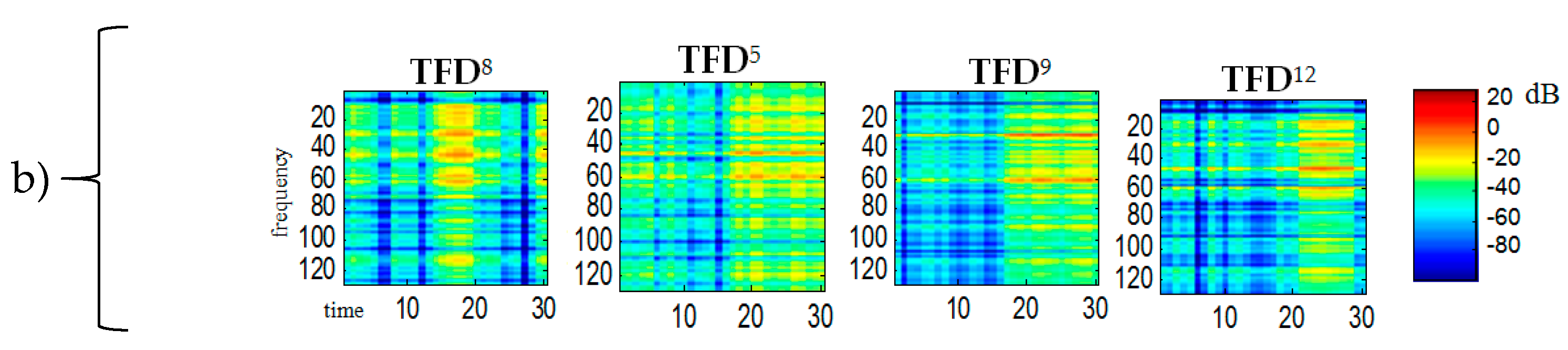
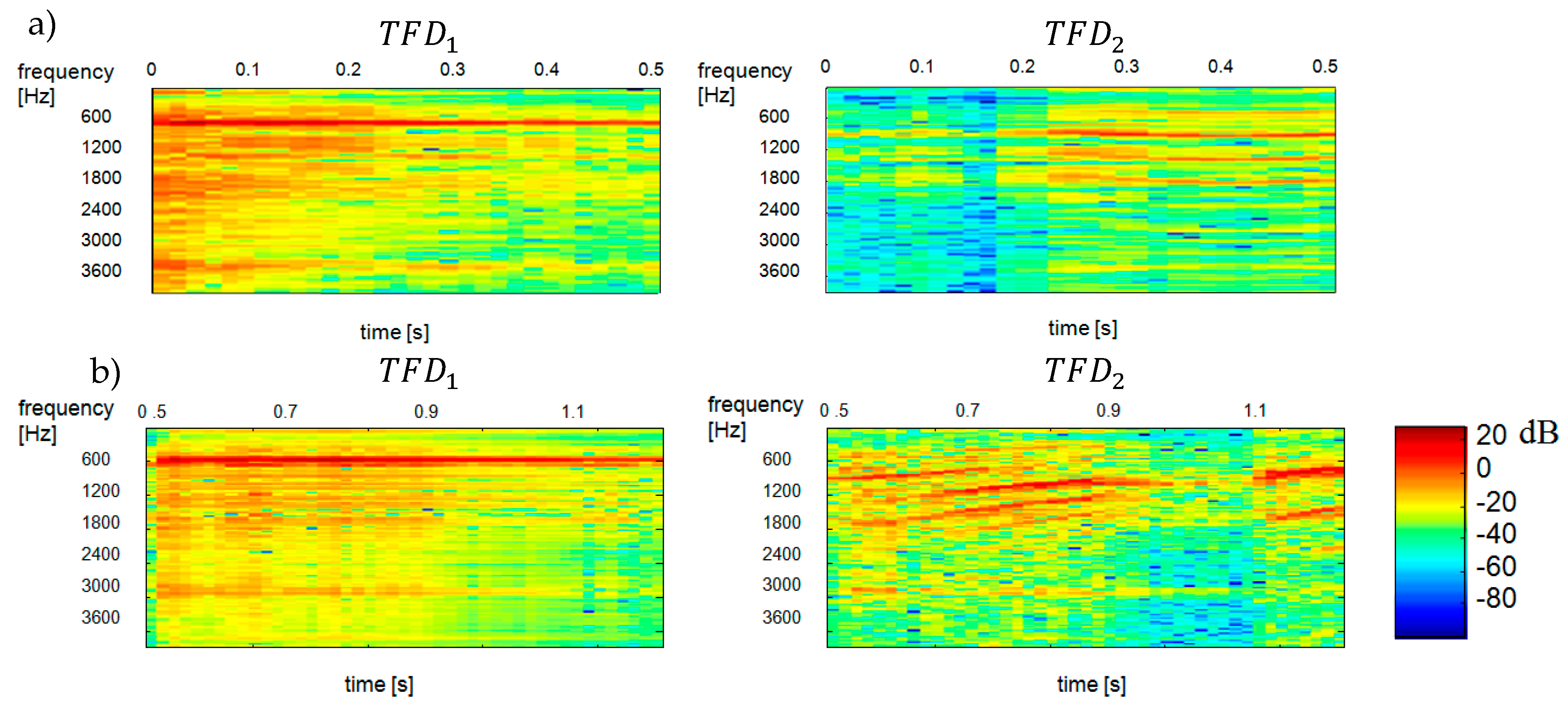
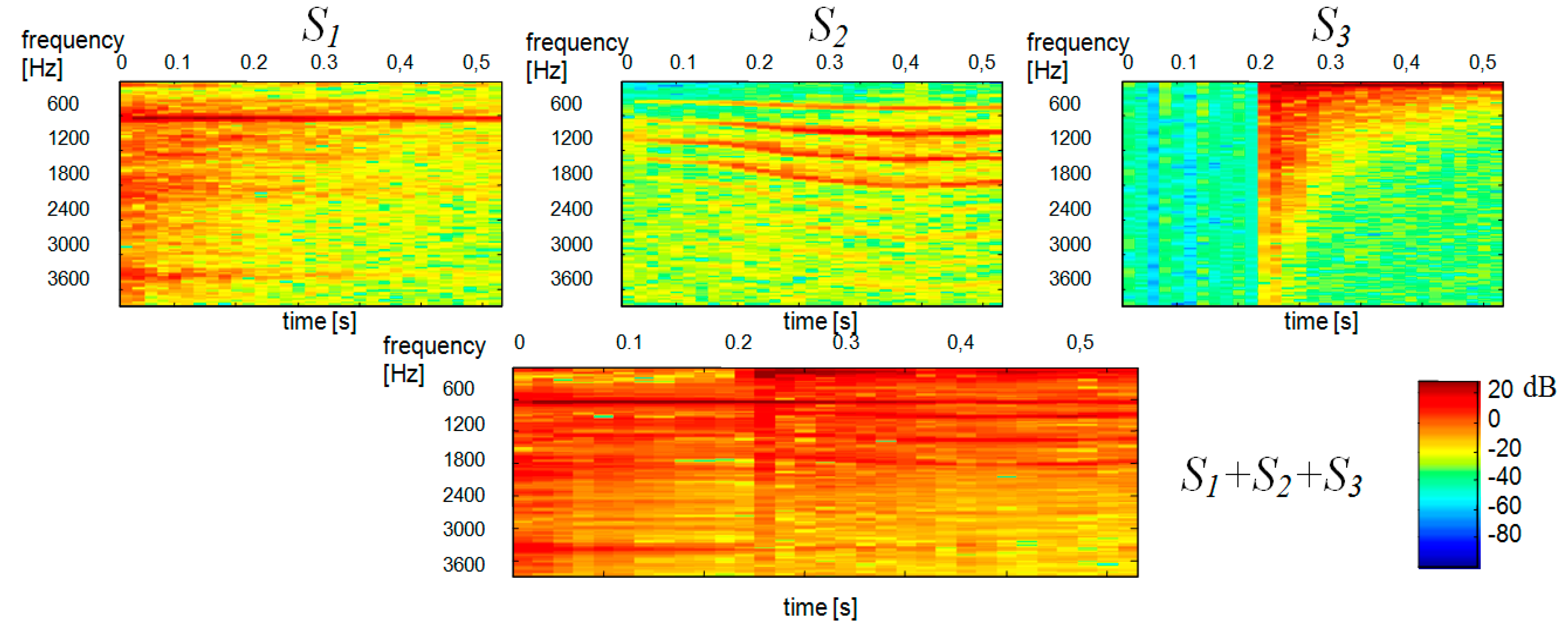
The proposed idea of single channel separation was verified by experimental tests. The experiments involved demixing single-channel signal consisting of two and three constituent signals. The constituent signals , and were selected so that their spectral composition and their respective types of sources were different. The signal (“ringer”) was generated by an electric device and was a recording of an electric ringer, while the signal (”baby”) was a baby cry, which means that it had a specific stochastic variation of the spectre, as do all sounds generated by living beings. The signal (“tom”) was a sound generated by a percussion instrument and, as such, was a typical impulsive signal. The above constituent signals were mixed in the following combinations: and . The signals were recorded at the sampling frequency and their duration was 1.2 s. Mixed single channel signal was transformed to the frequency domain using the STFT. We use blocks 256 samples long, 50% overlapped. The t-f analysis was performed in two separate blocks of 3968 and 5888 samples corresponding to the time intervals of 0–0.51 s and 0.51–1.2 s, respectively, in order to ensure higher stationarity of signal spectra in individual blocks. We used full signals of 9856 samples to determine the distance. Figure 2 shows the spectrograms of constituent signals and , with the spectrogram on the left showing the signal (“ringer”) and the spectrogram on the right showing the signal (“baby”).
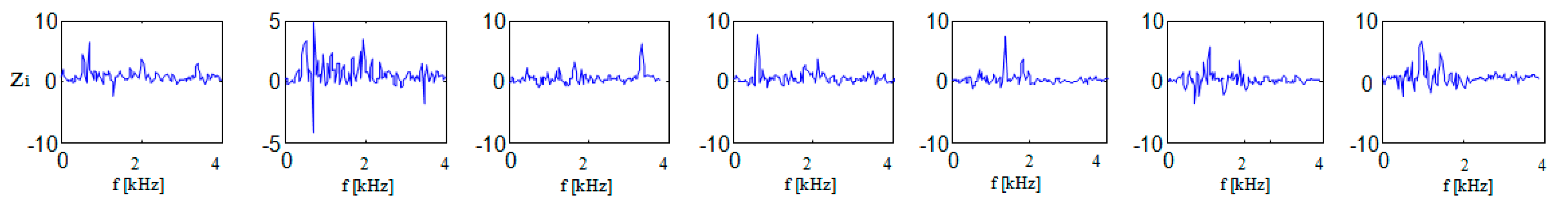
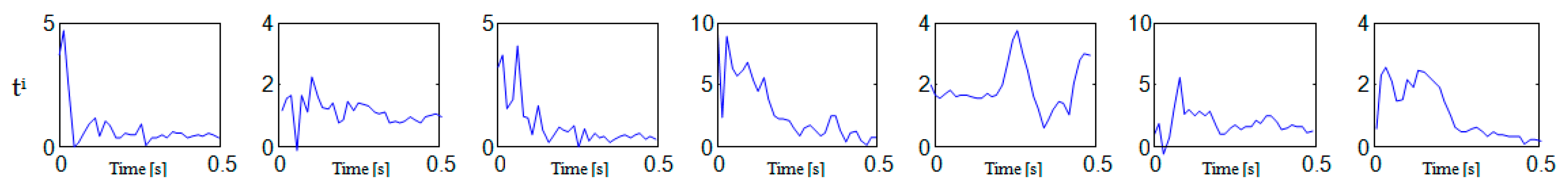
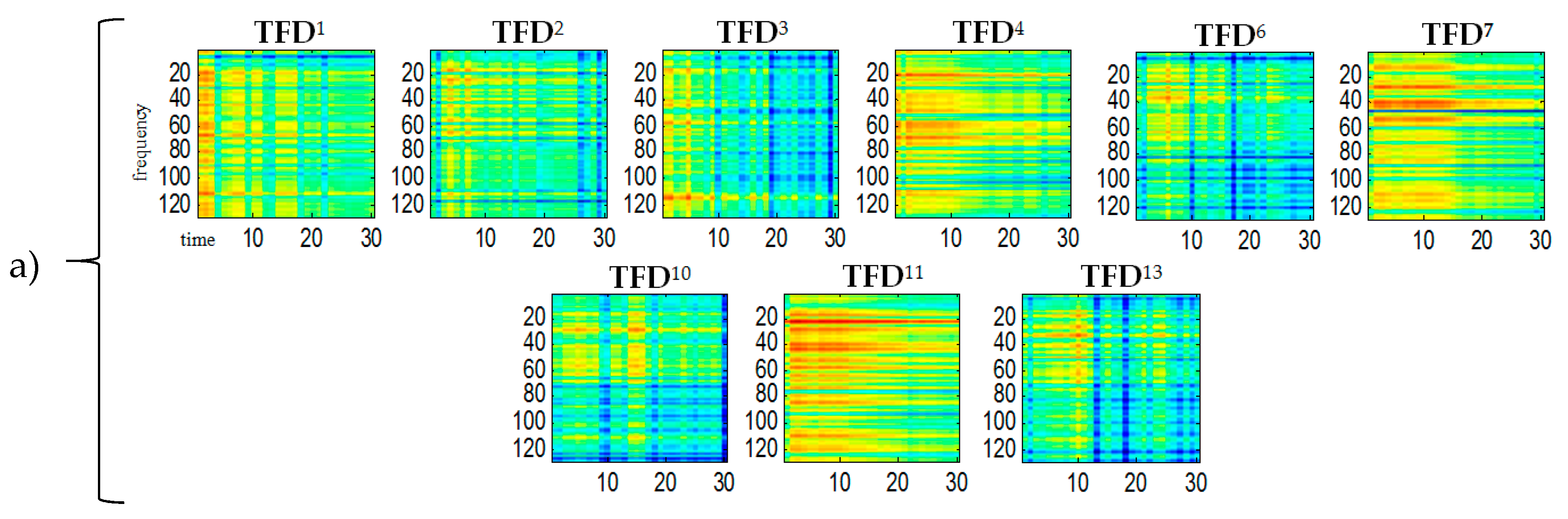
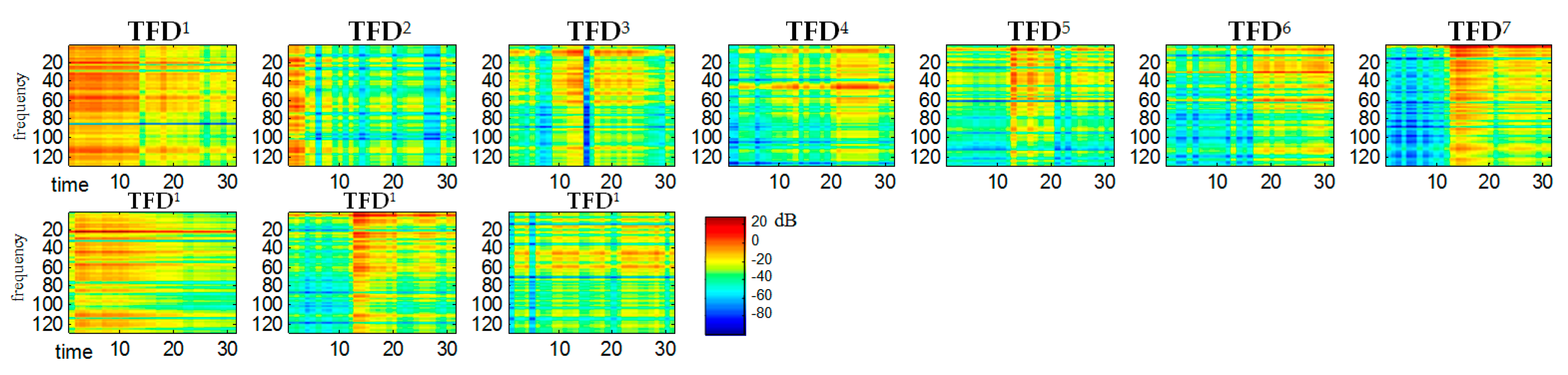
The STFT-generated spectrogram of (bottom diagram in Figure 2) was treated as a multichannel signal and estimated by ICA. This was done using the FastICA Matlab function algorithm based on [14]. Signal whitening was performed by singular value decomposition (SVD) using the Matlab function svd. ICA-generated statistically independent spectral bases , time bases and time-frequency bases for the variance of the input signal are shown in Figure 3, Figure 4 and Figure 5, respectively.
For all shown in the Figure 5 the ordinate axes scales range 0–129, which corresponds to the frequency range 0–4 kHz. The time scale range 0–30 corresponds to the range 0–0.51 s. A comparison of the obtained bases in Figure 2 reveals that bases 4, 7, 11 belong to the spectrogram of the S1 signal (ringer). Both this figure and some subsequent figures show the ICA results made in the first sample block (from 0 to 0.51 s).
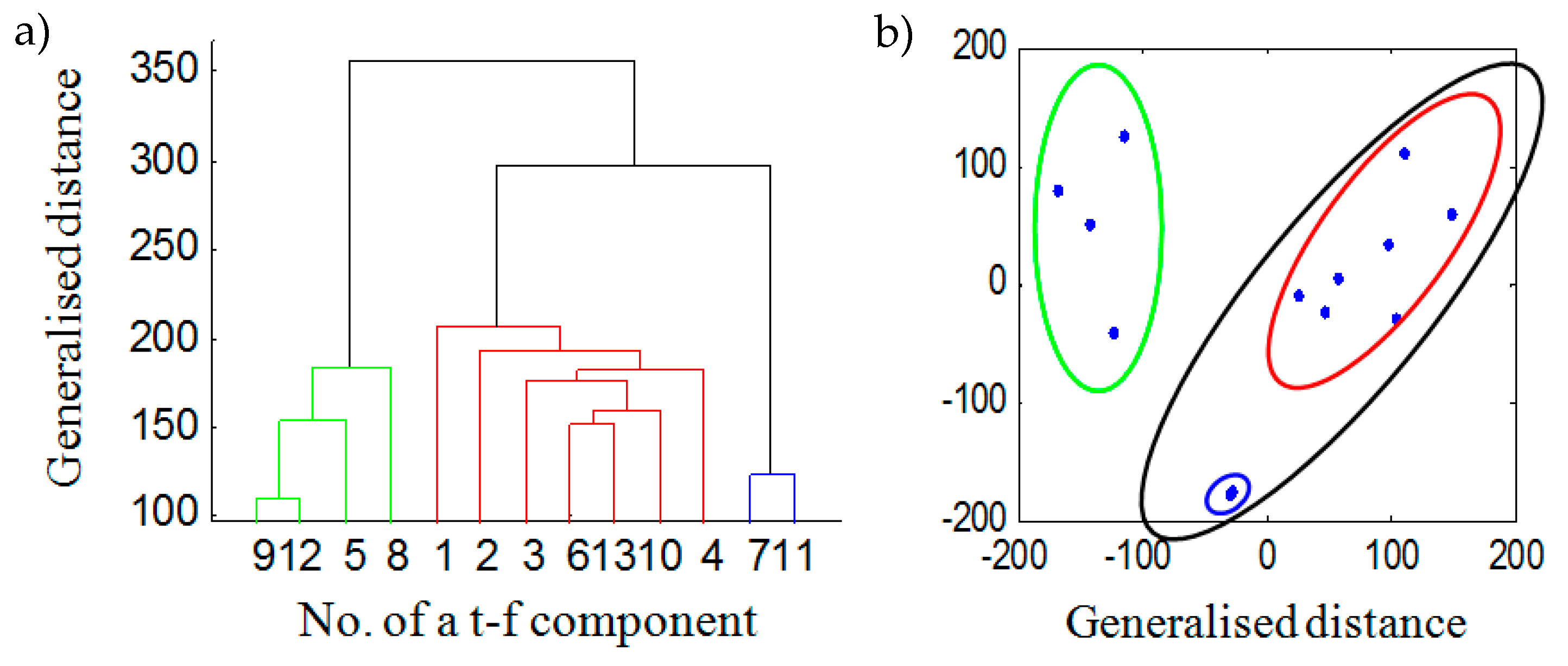
The clustering was performed by hierarchical [48] and k-mean partitional clustering [52] using two standard Matlab functions: dendrogram and kmeans. Figure 6a shows the separation results obtained with the Euclidean distance between components and a dendrogram obtained by hierarchical clustering. Figure 6b illustrates the “distances” between components obtained by multidimensional scaling [53]. Ellipses correspond to components collected in the dendrogram shown in Figure 6a. By summing the components grouped in Figure 6b and shown as green and black ellipses, we obtain spectrograms of two separated components seen in Equation (15):
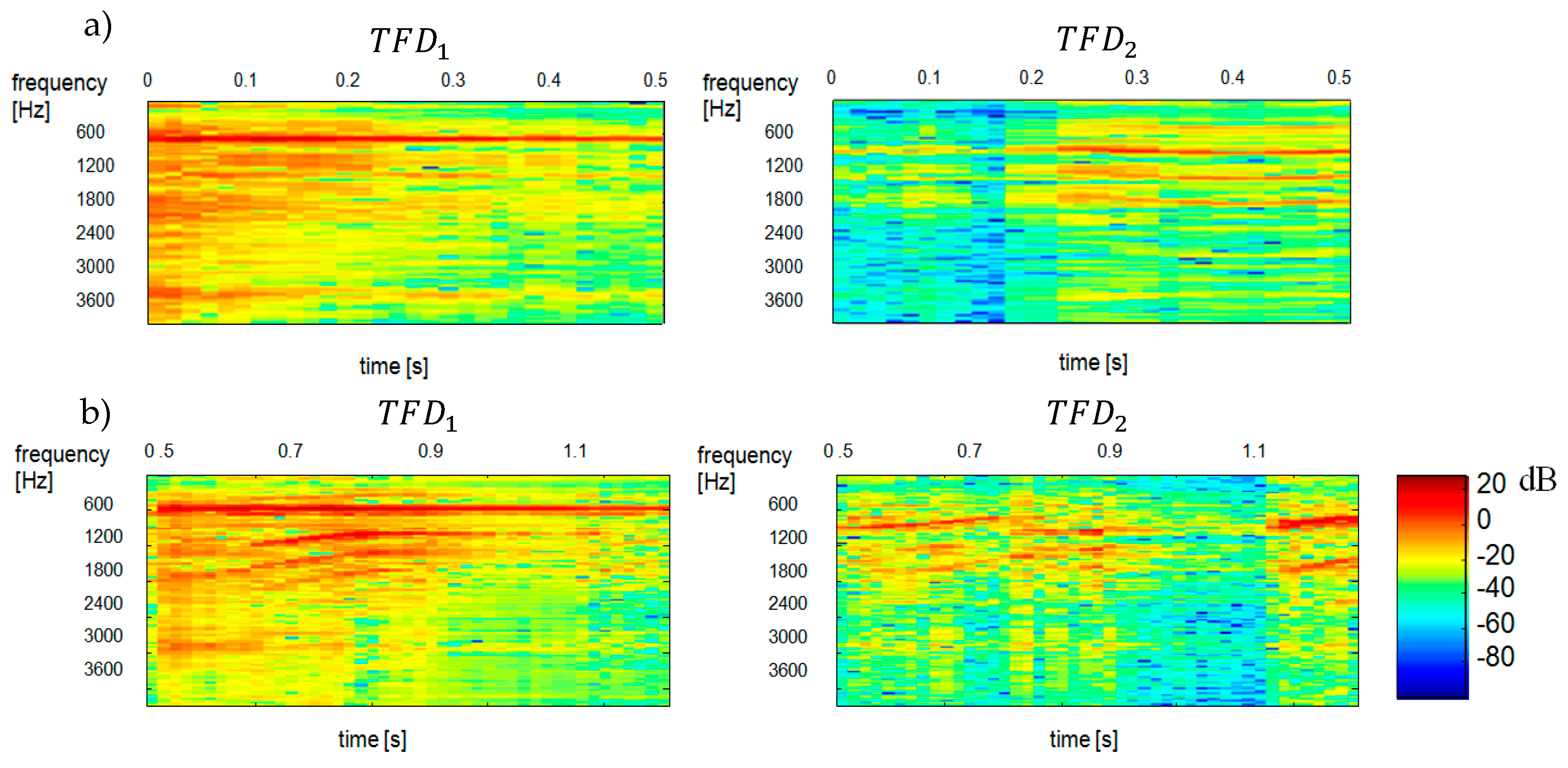
Figure 7 shows the reconstructed spectrograms of and components. Figure 8 shows the results of separation obtained by maximizing the negentropy of components and .
An analysis of the data in Figure 9 demonstrates that the separation is effective yet it depends on the length and the variance (parameter ) of the analysed signal, and hence on the number of obtained bases. The lower the number of these bases is, the more effective the grouping results are obtained. Nevertheless, a decrease in the variance results in a reduced quality of reconstruction spectrograms. The quality of separation is considerably lower for the variance of the mixed signal, which is manifested in the interpenetration (interference) of spectra of the constituent signals.
Figure 9 shows the results of clustering process with β distance of Gaussian distribution . As it results from the presented Figure 9 results of the separation seems to be efficient. They depend however on the length of the analysed signal and the used variance value of the analysed signal (parameter α) and therefore on the number of received bases. The smaller the number, the better the grouping results. However, lowering the value of variance α also causes a reduction in the quality of spectrogram reconstruction. The quality of separation is significantly worse when using variance of the mixed signal, which is manifested by the interpenetration (interference) of spectra of the signal components.
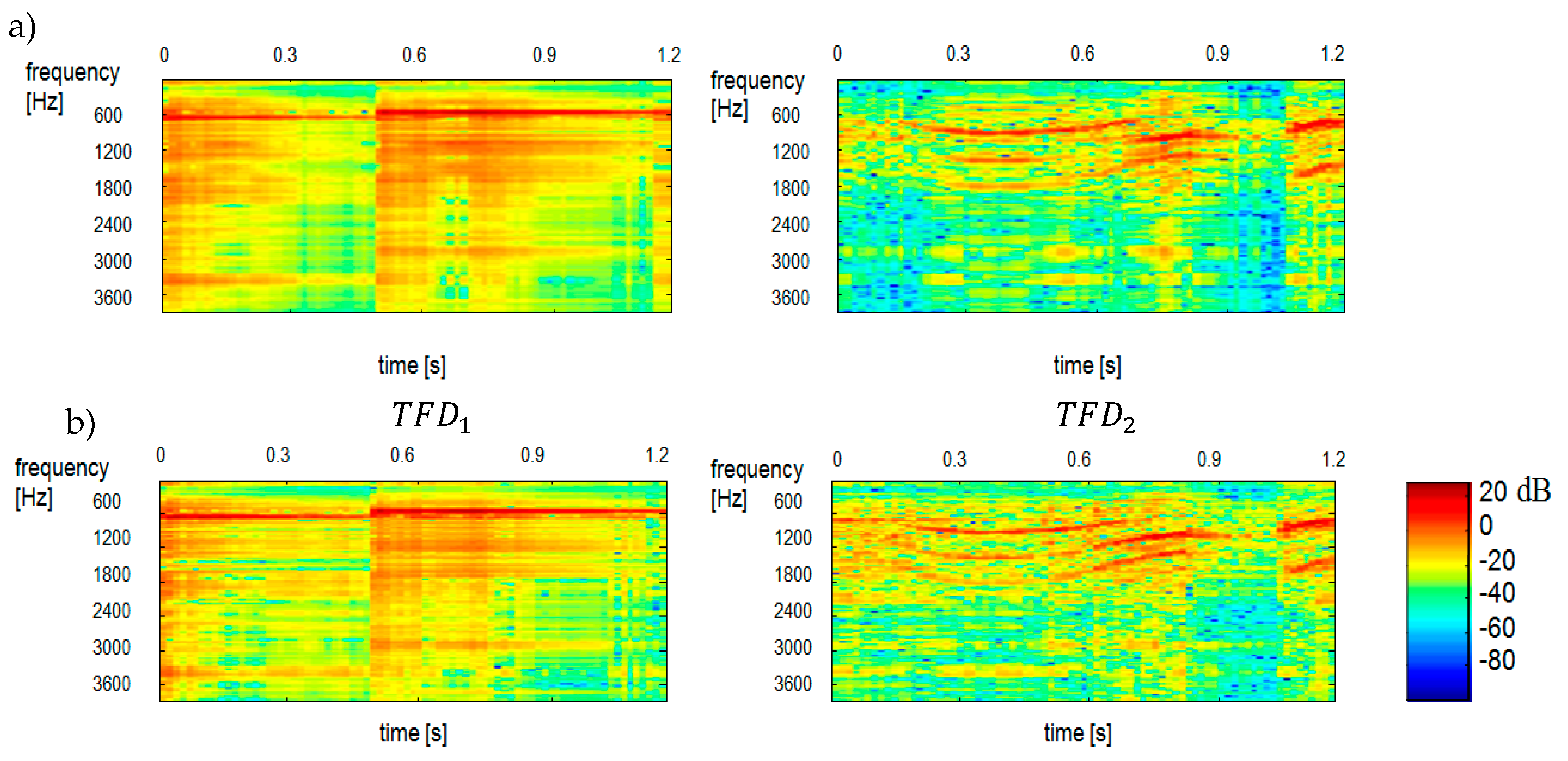
We used our method for the demixing a single-channel signal consisting of three component signals . The spectrogram of the mixed signal as well as the spectrograms of its constituent signals were shown in Figure 10. Like in Figure 5 the scales range 0–129 for all corresponds to the frequency range 0–4 kHz. The time scale range 0–30 corresponds to the range 0–0.51 s. Statistically independent bases are shown in Figure 11. One can notice a sharp similarity between bases and the constituent sounds of the mixed signal. To give an example, , , are ringer sounds, , and are tom sounds, while other bases are baby sounds. Hence, at the clustering stage, the bases were grouped into 3 classes (clusters) by k-mean partitional clustering. Figure 12 shows the results of separation of a three-component signal.
4. Perceptual Evaluation
For each of the decomposition versions presented in Section 3, the inverse STFT for every separated was used. The proposed separation method has been implemented in Matlab. The inverse STFT involved reconstructing time signals based on the spectrograms of separated bases. Given that such transformation is only based on amplitude information (spectrograms do not contain phase information), the time signals were additionally burdened with the error of “imprecise” invertibility of the STFT. In order to eliminate the effect of “imperfect” invertibility of the STFT (phase distortion), the reference signal’s sounds of the mix were also re-synthesized with zero phase. The RMS values of all separated and reference signals were normalised. All sounds were Microsoft Windows system sounds and were resampled to 8 kHz.
For the purpose of the test, 9 pairs of reference (original) and separated sound were prepared. These pairs are called “samples”. We generated 5 sets of samples (one set per every listener), each containing 9 samples. Sequence of samples was random and different in each set. The samples were separated by 3 to 4 s of silence. Each of five participants listened to five sets of samples. The participants included one sound engineer, two instrumental musicians and two individuals not related to music. Every listener listened to samples at the same loudness (over 80 dBA) over the AKG K271 closed-back (studio) headphones in studio room. Degradation category rating scale [54] was used to rate the quality of separation by the listener. The original five-point scale was extended to six-point, as suggested by the listeners. A score of 1 means “very distorted” while a score of 6 means “inaudibly distorted”. Before the final test, each listener underwent a short training session.
Table 1 gives the scores (mean values and standard deviations) of perceptual quality of separation with distance of Gaussian distribution and the Euclidean distance for components. Table 2 shows the impact of the mixed signal variance used ( or ) on the perceptual quality of separation.
The best results were obtained for the separation performed with the use of the distance. The ringer sound was most efficiently unmixed for every mixed signal type and distance measure. The results of the baby sound are worse. The tom sound was the most difficult to separate. These results demonstrate that the proposed method is the most effective for signals (sounds) with a quasi-stationary signals with harmonic spectrum (ringer) and the least effective for non-stationary signals with a noise-like spectrum (tom). The quality of separation is higher when the variance of the mixed signal is higher (Table 2) and, as expected, when separating from two-component mixes. In this case, specifically, the results are 0.5 points higher on the average.
5. Computational Complexity and Comparison Analysis
In this section, we evaluate the computational complexity of the proposed methods and compare our results with those obtained by other simple single-channel source separation methods. Our approach consists of five stages of processing: transformation of the time signal into a spectrogram, ICA stage with whitening as pre-processing, calculation of distance measure, grouping and inverse transform to the time domain. We consider the approximate number of floating point operations (flops). The code is implemented on a 2.8 GHz (CPU), 8 GHz (RAM) platform. At the transformation stage, we employ STFT with the FFT algorithm which is a very effective method because it involves overall (only the most significant terms are retained) flops for the time window (time segment), where 2n is the number of samples in the time window used in STFT. Using the big notation, the computational complexity of this stage is . In the ICA stage, we used the Singular Value Decomposition (SVD) as pre-processing which involves flops, where is the number of time segments used in STFT stage. At the SVD sub-stage, we reduced the dimension of the analysis based on the desired signal variance value . In the ICA stage, we used the FastICA algorithm which is a very effective algorithm and requires only [55] per iteration, where is a dimension of ICA reduced in the SVD sub-stage. This means that the approximation of complexity in the ICA stage is of order . In the stage of calculating the distance between the bases we used two types of distances: the classic Euclidean distance and the distance , that require approximately and flops, respectively. In the clustering stage, we used the hierarchical clustering algorithm (single-linkage type) or the k-mean algorithm. Both algorithms have computational complexity of order [48] but it includes the complexity of distances and calculating as the main stage of clustering process. At the inverse transform stage, we used IFFT algorithm which requires, similar to FFT, flops.
In order to compare our method with others solutions, we additionally carry out single-channel separation using the method proposed in [19] and the method based on analysing the similarity of time bases which are called here as TFD-SCSS, KL-SCSS and T-SCSS, respectively. In the KL-SCSS method, the Kullback–Leibler distance (symmetrical Kullback–Leibler divergence) is used as a measure of distance for the spectral bases . In the T-SCSS method we use the Euclidean distance for time bases . Separation efficiency is measured using the root mean square error indicator (RMSE) compared to the original sources. Considering the spectrograms of the original sources and separate sources, the RMSE is calculated as:
where are the row and column indices of the and indices.
The same set of source and mixed signals as in the auditory tests (Section 4) as well as the same analysis parameters are used in the comparative analysis. Table 3 presents the average results of the RMSE index for four combinations of mixed signals. It can be stated that our method based on the time and frequency domain similarity generally yields better separation results than those obtained with the methods that only use time or spectral similarity. For the mixed signal ringer + tom, better separation results are obtained using T-SCSS. This probably results from the clear differences in the time structure of the signal sources and better matching of distance in the T-SCSS method.
In addition, the time-course results are subjected to auditory testing. Table 4 gives the scores (mean values and standard deviations) of the perceptual quality of separation of our methods with the distance of the Gaussian distribution and the KL-SCSS and T-SCSS methods.
6. Conclusions
This study proposed a new ICA-based method for single channel separation in time-frequency domain. In terms of the grouping of bases and distance measure types, the methods can be divided into those which require some information about the source signals (the distance) and those which only exploit the similarity between bases (Euclidean distance and negentropy minimization). The aim should be to group the bases without the use of any information about constituent signals. Nevertheless, the selection of a distance depends on the constituent signals , which means that some information about the mixed signal is required. If the signal amplitude varies in time to a significant extent, the Euclidean distance should be employed. This distance is by nature predisposed to group the spectral and time features of a signal. It has been shown that clustering analysis (in hierarchical and k-means forms) can be effectively used to group basis components of the signals. In order for the decomposition to be successful, the source components of mixed signals should have a stationary spectrum in the analysed period. Although this limitation can be overcome by shortening the analysed period, it causes in the deterioration in audible quality of reconstructed signals. The main limitation of the method is the lack of universality of the procedure. The selection of a distance measure and a clustering algorithm depends on the time-frequency structure of component signals of the mix. In addition to that, the results of separation greatly depend on the variance parameter . If a value of is too high and thus the number of bases is high too, the clustering will yield worse results. This is caused by the scattering of characteristics of the constituent signal spectra with a greater number of bases. On the other hand, if a value of is too low, the quality of reconstructed signal spectra will be lower too. The quality of separation also depends on ICA limitations. As the number of mixed signals increases, the quality of separated component signals decreases, which is evidenced in the interpenetration of the component signal spectra.
Author Contributions
Conceptualization, G.B., D.M., J.J.; formal analysis, J.J.; funding acquisition, J.J.; investigation, J.J.; methodology, D.M., G.B.; project administration, J.J.; resources, D.M.; software, D.M.; supervision, J.J.; validation, J.J.; visualization, D.M.; writing—review and editing J.J. All authors provided critical feedback and collaborated in the research. All authors have read and agreed to the published version of the manuscript.
Funding
The project/research was financed in the framework of the project Lublin University of Technology; Regional Excellence Initiative, funded by the Polish Ministry of Science and Higher Education (contract no.030/RID/2018/19).
Conflicts of Interest
The authors declare no conflict of interest.
References
- Al-Baddai, S.; Al-Subari, K.; Tomé, A.M.; Volberg, G.; Lang, E.W. Combining EMD with ICA to Analyze Combined EEG-fMRI Data. In Proceedings of the MIUA, Egham, UK, 9–11 July 2014; pp. 223–228. [Google Scholar]
- James, C.J.; Hesse, C.W. Independent component analysis for biomedical signals. Physiol. Meas. 2005, 26, R15–R39. [Google Scholar] [CrossRef]
- Jimenéz-Gonzaléz, A.; James, C. Source separation of Foetal Heart Sounds and maternal activity from single-channel phonograms: A temporal independent component analysis approach. In Proceedings of the 2008 Computers in Cardiology, Bologna, Italy, 14–17 September 2008; pp. 949–952. [Google Scholar]
- Zeng, X.; Li, S.; Li, G.J.; Zhou, Y.; Mo, D.H. Fetal ECG extraction by combining single-channel SVD and cyclostationarity-based blind source separation. Int. J. Signal Process 2013, 6, 367–376. [Google Scholar]
- Draper, B.A.; Baek, K.; Bartlett, M.S.; Beveridge, J.R. Recognizing faces with PCA and ICA. Comput. Vis. Image Underst. 2003, 91, 115–137. [Google Scholar] [CrossRef]
- Liu, X.; Srivastava, A.; Gallivan, K. Optimal Linear Representations of Images for Object Recognition. In Proceedings of the 2003 Conference on Computer Vision and Pattern Recognition Workshop, Madison, WI, USA, 18–20 June 2003. [Google Scholar]
- Yang, J.; Williams, D.B. MIMO Transmission Subspace Tracking with Low Rate Feedback. In Proceedings of the IEEE International Conference on Acoustics, Speech, and Signal Processing, Philadelphia, PA, USA, 23 March 2005. [Google Scholar]
- Wilson, S.; Yoon, J. Bayesian ICA-based source separation of Cosmic Microwave Background by a discrete functional approximation. arXiv 2010, arXiv:1011.4018. [Google Scholar]
- Eronen, A. Musical Instrument Recognition Using ICA-Based Transform of Features and Discriminatively Trained HMMs. In Proceedings of the Seventh International Symposium on Signal Processing and Its Applications, Paris, France, 4 July 2003. [Google Scholar]
- Hyvarinen, A.; Karhunen, J.; Oja, E. Independent Component Analysis; John Wiley & Sons: New York, NY, USA, 2001. [Google Scholar]
- Amari, S.-I. Natural gradient learning for over- and under-complete bases in ICA. Neural Comput. 1999, 11, 1875–1883. [Google Scholar] [CrossRef]
- Lewicki, M.S.; Sejnowski, T.J. Learning Nonlinear Overcomplete Representations for Efficient Coding. In Proceedings of the Advances in Neural Information Processing Systems, Denver, CO, USA, 30 November–5 December 1998; pp. 556–562. [Google Scholar]
- Birtea, P.; Caşu, I.; Comănescu, D. First order optimality conditions and steepest descent algorithm on orthogonal Stiefel manifolds. Optim. Lett. 2018, 13, 1773–1791. [Google Scholar] [CrossRef] [Green Version]
- Edelman, A.; Arias, T.A.; Smith, S.T. The Geometry of Algorithms with Orthogonality Constraints. SIAM J. Matrix Anal. Appl. 1998, 20, 303–353. [Google Scholar] [CrossRef]
- Mika, D.; Jozwik, J. Lie Group Methods in Blind Signal Processing. Sensors 2020, 20, 440. [Google Scholar] [CrossRef] [Green Version]
- Pecora, A.; Maiolo, L.; Minotti, A.; De Francesco, R.; De Francesco, E.; Leccese, F.; Cagnetti, M.; Ferrone, A. Strain Gauge Sensors Based on Thermoplastic Nanocomposite for Monitoring Inflatable Structures. In Proceedings of the 2014 IEEE Metrology for Aerospace (MetroAeroSpace), Benevento, Italy, 29–30 May 2014. [Google Scholar]
- Petritoli, E.; Leccese, F.; Leccisi, M. Inertial Navigation Systems for UAV: Uncertainty and Error Measurements. In Proceedings of the 2019 IEEE 5th International Workshop on Metrology for AeroSpace (MetroAeroSpace), Torino, Italy, 19–21 June 2019; pp. 1–5. [Google Scholar]
- Lee, T.W.; Lewicki, M.S. The Generalized Gaussian Mixture Model Using ICA. In Proceedings of the International Workshop on Independent Component Analysis (ICA’00), Helsinki, Finland, 19–22 June 2000; pp. 239–244. [Google Scholar]
- Casey, M.A.; Westner, A. Separation of Mixed Audio Sources By Independent Subspace Analysis. In Proceedings of the ICMC, Berlin, Germany, 27 August–1 September 2000; pp. 154–161. [Google Scholar]
- Jang, G.J.; Lee, T.W. A maximum likelihood approach to single-channel source separation. J. Mach. Learn. Res. 2003, 4, 1365–1392. [Google Scholar]
- Barry, D.; Fitzgerald, D.; Coyle, E.; Lawlor, B. Single Channel Source Separation Using Short-Time Independent Component Analysis. In Proceedings of the 119th Audio Engineering Society Convention, New York, NY, USA, 7–10 October 2005. [Google Scholar]
- Barry, D.; Lawlor, B.; Coyle, E. Sound Source Separation: Azimuth Discrimination and Resynthesise. In Proceedings of the 7th International Conference on Digital Audio Effects, DAFX 04, Naples, Italy, 5–8 October 2004. [Google Scholar]
- Cooney, R.; Cahill, N.; Lawlor, R. An Enhanced Implementation of the ADRess (Azimuth Discrimination and Resynthesis) Music Source Separation Algorithm. In Proceedings of the 121st Audio Engineering Society Convention, San Francisco, CA, USA, 6–8 October 2006. [Google Scholar]
- Master, A.S. Stereo Music Source Separation via Bayesian Modeling. Ph.D. Thesis, Stanford University, Stanford, CA, USA, 2006. [Google Scholar]
- Vinyes, M.; Bonada, J.; Loscos, A. Demixing Commercial Music Productions via Human-Assisted Time-Frequency Masking. In Proceedings of the Audio Engineering Society 120th Convention, Paris, France, 20–23 May 2006. [Google Scholar]
- Wang, D.; Brown, G. Computational Auditory Scene Analysis; Institute of Electrical and Electronics Engineers: Piscataway, NJ, USA, 2006. [Google Scholar]
- Bach, F.R.; Jordan, M.I. Blind One-Microphone Speech Separation: A Spectral Learning Approach. In Proceedings of the Advances in Neural Information Processing Systems, Vancouver, BC, Canada, 13–18 December 2004; pp. 65–72. [Google Scholar]
- Yilmaz, O.; Rickard, S. Blind Separation of Speech Mixtures via Time-Frequency Masking. IEEE Trans. Signal Process. 2004, 52, 1830–1847. [Google Scholar] [CrossRef]
- RIckard, S.; Yilmaz, O. On the Approximate W-Disjoint Orthogonality of Speech. In Proceedings of the 2002 IEEE International Conference on Acoustics, Speech, and Signal Processing, Orlando, FL, USA, 13–17 May 2002. [Google Scholar]
- Brungart, D.S.; Chang, P.S.; Simpson, B.D.; Wang, D. Isolating the energetic component of speech-on-speech masking with ideal time-frequency segregation. J. Acoust. Soc. Am. 2006, 120, 4007–4018. [Google Scholar] [CrossRef] [PubMed] [Green Version]
- Jang, G.-J.; Lee, T.-W.; Oh, Y.-H. Learning statistically efficient features for speaker recognition. Neurocomputing 2002, 49, 329–348. [Google Scholar] [CrossRef]
- Taghia, J.; Doostari, M.A. Subband-based single-channel source separation of instantaneous audio mixtures. World Appl. Sci. J. 2009, 6, 784–792. [Google Scholar]
- Davies, M.E.; James, C. Source separation using single channel ICA. Signal Process. 2007, 87, 1819–1832. [Google Scholar] [CrossRef]
- Wang, B.; Plumbley, M.D. Investigating Single-Channel Audio Source Separation Methods Based on Non-Negative Matrix Factorization. In Proceedings of the ICA Research Network International Workshop, Liverpool, UK, 18–19 September 2006; pp. 17–20. [Google Scholar]
- Mijović, B.; De Vos, M.; Gligorijević, I.; Taelman, J.; Van Huffel, S. Source Separation From Single-Channel Recordings by Combining Empirical-Mode Decomposition and Independent Component Analysis. IEEE Trans. Biomed. Eng. 2010, 57, 2188–2196. [Google Scholar] [CrossRef]
- Litvin, Y.; Cohen, I. Single-Channel Source Separation of Audio Signals Using Bark Scale Wavelet Packet Decomposition. J. Signal Process. Syst. 2010, 65, 339–350. [Google Scholar] [CrossRef]
- Duan, Z.; Zhang, Y.; Zhang, C.; Shi, Z. Unsupervised Single-Channel Music Source Separation by Average Harmonic Structure Modeling. IEEE Trans. Audio Speech Lang. Process. 2008, 16, 766–778. [Google Scholar] [CrossRef]
- Rapaport, G. Codebook-Based Single-Channel Blind Source Separation of Audio Signals; Technion-Israel Institute of Technology, Faculty of Electrical Engineering: Hajfa, Israel, 2011. [Google Scholar]
- Gao, B. Single Channel Blind Source Separation. Ph.D. Thesis, Newcastle University, Newcastle, UK, 2011. [Google Scholar]
- Hyvärinen, A.; Pajunen, P. Nonlinear independent component analysis: Existence and uniqueness results. Neural Netw. 1999, 12, 429–439. [Google Scholar] [CrossRef]
- Jutten, C.; Karhunen, J. Advances in blind source separation (BSS) and independent component analysis (ICA) for nonlinear mixtures. Int. J. Neural Syst. 2004, 14, 267–292. [Google Scholar] [CrossRef]
- Isomura, T.; Toyoizumi, T. On the achievability of blind source separation for high-dimensional nonlinear source mixtures. arXiv 2018, arXiv:1808.00668. [Google Scholar]
- Mika, D.; Jozwik, J. Advanced Time-Frequency Representation in Voice Signal Analysis. Adv. Sci. Technol. Res. J. 2018, 12, 251–259. [Google Scholar] [CrossRef]
- Mika, D.; Jozwik, J. Normative measurements of noise at cnc machines work stations. Adv. Sci. Technol. Res. J. 2016, 10, 138–143. [Google Scholar] [CrossRef]
- Mika, D. Separation of Sounds from Various Sources in a Mixed Acoustic Signal. Ph.D. Thesis, AGH University, Cracow, Poland, 2011. [Google Scholar]
- Mika, D.; Kleczkowski, P. ICA-based Single Channel Audio Separation: New Bases and Measures of Distance. Arch. Acoust. 2011, 36, 311–331. [Google Scholar] [CrossRef] [Green Version]
- Jain, A.K.; Murty, M.N.; Flynn, P.J. Data clustering: A review. ACM Comput. Surv. 1999, 31, 264–323. [Google Scholar] [CrossRef]
- Jain, A.K.; Murty, M.N.; Flynn, P.J. Algorithms for Clustering Data; Prentice-Hall Advanced Reference Series; Prentice-Hall, Inc.: New York, NY, USA, 1988. [Google Scholar]
- Box, G.E.P.; Tiao, G.C. Bayesian Inference in Statistical Analysis; John Wiley & Sons: New York, NY, USA, 2011. [Google Scholar]
- Cover, T.M.; Thomas, J.A. Elements of Information Theory; John Wiley & Sons: New York, NY, USA, 2012. [Google Scholar]
- Petritoli, E.; Leccese, F. High Accuracy Attitude and Navigation System for an Autonomous Underwater Vehicle (AUV). Acta IMEKO 2018, 7, 3–9. [Google Scholar] [CrossRef]
- Macqueen, J. Some Methods for Classification and Analysis of Multivariate Observations; University of California Press: Berkeley, CA, USA, 1967; pp. 281–297. [Google Scholar]
- Seber, G.A.F. Multivariate Observations; John Wiley & Sons: New York, NY, USA, 2009. [Google Scholar]
- Bech, S.; Zacharov, N. Perceptual Audio Evaluation-Theory, Method and Application; Wiley: Hoboken, NJ, USA, 2006. [Google Scholar]
- Zarzoso, V.; Comon, P.; Kallel, M. How Fast is FastICA? In Proceedings of the 2006 14th European Signal Processing Conference, Florence, Italy, 4–8 September 2006; pp. 1–5. [Google Scholar]
Figure 1.
Block diagram of standard independent component analysis.

Figure 2.
Spectrograms of constituent signals, (a) S1—ringer; (b) S2—baby and (c) the mixed signal S1 + S2.
Figure 2.
Spectrograms of constituent signals, (a) S1—ringer; (b) S2—baby and (c) the mixed signal S1 + S2.

Figure 3.
7 spectral bases obtained by ICA on the spectrogram of the mixed signal for variance .

Figure 4.
7 time bases obtained by ICA on the spectrogram of the mixed signal for variance .

Figure 5.
13 statistically-independent bases obtained by ICA on the spectrogram of the mixed signal for a signal variance : (a) bases belonging for S1 source (b) bases belonging for S2 source.
Figure 5.
13 statistically-independent bases obtained by ICA on the spectrogram of the mixed signal for a signal variance : (a) bases belonging for S1 source (b) bases belonging for S2 source.


Figure 6.
The results of hierarchical clustering for the Euclidean distance for components (a), and visualisation of groups of obtained by multidimensional scaling (b).
Figure 6.
The results of hierarchical clustering for the Euclidean distance for components (a), and visualisation of groups of obtained by multidimensional scaling (b).

Figure 7.
Reconstructed spectrograms (spectra) of and components as a results of hierarchical clustering with Euclidean distance for components. —ringer, —baby: (a) results for the time interval of 0.00–0.51 s, (b) results for the time interval of 0.51–1.20 s.
Figure 7.
Reconstructed spectrograms (spectra) of and components as a results of hierarchical clustering with Euclidean distance for components. —ringer, —baby: (a) results for the time interval of 0.00–0.51 s, (b) results for the time interval of 0.51–1.20 s.

Figure 8.
Reconstructed spectrograms (spectra) of and components obtained by minimizing the negentropy of and components. —ringer, —baby: (a) results for the time interval of 0.00–0.51 s, (b) results for the time interval of 0.51–1.20 s.
Figure 8.
Reconstructed spectrograms (spectra) of and components obtained by minimizing the negentropy of and components. —ringer, —baby: (a) results for the time interval of 0.00–0.51 s, (b) results for the time interval of 0.51–1.20 s.

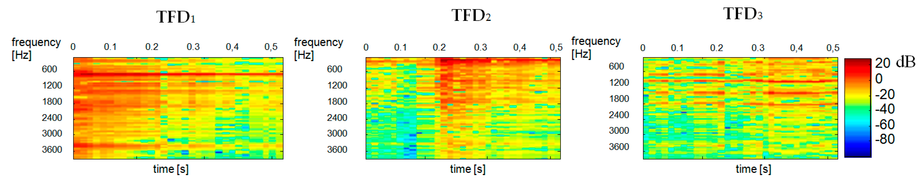
Figure 9.
Reconstructed spectrograms (spectra) of and components obtained by k-mean partitional clustering and the distance of Gaussian distribution. —ringer, —baby. The results were obtained for the variances (a) and (b) , respectively, and the signal duration of 1.2 s.
Figure 9.
Reconstructed spectrograms (spectra) of and components obtained by k-mean partitional clustering and the distance of Gaussian distribution. —ringer, —baby. The results were obtained for the variances (a) and (b) , respectively, and the signal duration of 1.2 s.

Figure 10.
Spectrograms of constituent signals: —ringer, —baby, —tom. The bottom spectrogram shows the mixed signal .
Figure 10.
Spectrograms of constituent signals: —ringer, —baby, —tom. The bottom spectrogram shows the mixed signal .

Figure 11.
Statistically independent bases of a three-component signal for the variance .

Figure 12.
Reconstructed spectrograms of a three-component signal obtained by k-mean partitional clustering and Euclidean distance for bases (duration: 0.51 s): —ringer, —tom, —baby.
Figure 12.
Reconstructed spectrograms of a three-component signal obtained by k-mean partitional clustering and Euclidean distance for bases (duration: 0.51 s): —ringer, —tom, —baby.


Table 1.
Results of test in the form of mean scores and standard deviations for each sound obtained with the Euclidean distance and the distance of Gaussian distribution for bases.
Table 1.
Results of test in the form of mean scores and standard deviations for each sound obtained with the Euclidean distance and the distance of Gaussian distribution for bases.
| Euclidean Distance | Distance | |
|---|---|---|
| baby | mean = 2.4400; σ = 0.9025 | mean = 3.4160; σ = 1.1158 |
| ringer | mean = 3.1200; σ = 1.0375 | mean = 4.4480; σ = 0.9875 |
| tom | mean = 2.5333; σ = 0.6644 | mean = 3.0500; σ = 0.7961 |
Table 2.
The impact of the mixed signal variance used on the perceptual quality of separation.
| Measure of Distance | “Ringer” | “Baby” | “Tom” | |||
|---|---|---|---|---|---|---|
| = 0.9 | = 0.7 | = 0.9 | = 0.7 | = 0.9 | = 0.7 | |
| distance | 5.00 | 4.36 | 4.32 | 3.04 | 2.75 | 2.14 |
| Euclidean distance | 3.44 | 4.00 | 2.44 | 2.64 | 2.42 | 1.63 |
Table 3.
RMSE index mean and standard deviation for separation algorithms used in comparative analysis.
Table 3.
RMSE index mean and standard deviation for separation algorithms used in comparative analysis.
| Separation Algorithm | RMSE (Mean and Std. dev.) | |||
|---|---|---|---|---|
| Baby + Ringer | Ringer + Tom | Baby + Tom | Baby + Ringer + Tom | |
| TFD-SCSS | 0.2120 ± 0.0235 | 0.1138 ± 0.0134 | 0.1821 ± 0.0148 | 0.3125 ± 0.0725 |
| KL-SCSS | 0.2935 ± 0.0455 | 0.3120 ± 0.0436 | 0.3120 ± 0.0445 | 0.5120 ± 0.1215 |
| T-SCSS | 0.2330 ± 0.0145 | 0.0820 ± 0.0212 | 0.2020 ± 0.0135 | 0.3520 ± 0.0935 |
Table 4.
Results of test in the form of mean scores and standard deviations for analysed methods.
| Source Signals | TFD-SCSS | KL-SCSS | T-SCSS |
|---|---|---|---|
| baby | mean = 3.4160; σ = 1.1158 | mean = 2.8420; σ = 1.3457 | mean = 3.2180; σ = 1.3651 |
| ringer | mean = 4.4480; σ = 0.9875 | mean = 3.8490; σ = 0.9961 | mean = 4.5460; σ = 0.9354 |
| tom | mean = 3.0500; σ = 0.7961 | mean = 2.7533; σ = 0.9832 | mean = 2.9544; σ = 0.8794 |
© 2020 by the authors. Licensee MDPI, Basel, Switzerland. This article is an open access article distributed under the terms and conditions of the Creative Commons Attribution (CC BY) license (http://creativecommons.org/licenses/by/4.0/).
Share and Cite
MDPI and ACS Style
Mika, D.; Budzik, G.; Józwik, J. Single Channel Source Separation with ICA-Based Time-Frequency Decomposition. Sensors 2020, 20, 2019. https://doi.org/10.3390/s20072019
AMA Style
Mika D, Budzik G, Józwik J. Single Channel Source Separation with ICA-Based Time-Frequency Decomposition. Sensors. 2020; 20(7):2019. https://doi.org/10.3390/s20072019
Chicago/Turabian StyleMika, Dariusz, Grzegorz Budzik, and Jerzy Józwik. 2020. "Single Channel Source Separation with ICA-Based Time-Frequency Decomposition" Sensors 20, no. 7: 2019. https://doi.org/10.3390/s20072019
Note that from the first issue of 2016, this journal uses article numbers instead of page numbers. See further details here.