Numerical Investigations on Wave Remote Sensing from Synthetic X-Band Radar Sea Clutter Images by Using Deep Convolutional Neural Networks

Abstract

X-band marine radar is an effective tool for sea wave remote sensing. Conventional physical-based methods for acquiring wave parameters from radar sea clutter images use three-dimensional Fourier transform and spectral analysis. They are limited by some assumptions, empirical formulas and the calibration process while obtaining the modulation transfer function (MTF) and signal-to-noise ratio (SNR). Therefore, further improvement of wave inversion accuracy by using the physical-based method presents a challenge. Inspired by the capability of convolutional neural networks (CNN) in image characteristic processing, a deep-learning inversion method based on deep CNN is proposed. No intermediate step or parameter is needed in the CNN-based method, therefore fewer errors are introduced. Wave parameter inversion models were constructed based on CNN to inverse the wave’s spectral peak period and significant wave height. In the present paper, the numerically simulated X-band radar image data were used for a numerical investigation of wave parameters. Results of the conventional spectral analysis and CNN-based methods were compared and the CNN-based method had a higher accuracy on the same data set. The influence of training strategy on CNN-based inversion models was studied to analyze the dependence of a deep-learning inversion model on training data. Additionally, the effects of target parameters on the inversion accuracy of CNN-based models was also studied.

1. Introduction

Sea wave remote sensing has important scientific significance and practical value [1]. Wave remote sensing is a fundamental part of ocean monitoring and helps to better understand the regular pattern of marine changes. It is also a key factor for safety assessment of offshore operations and real-time prediction of ship and platform motion attitude.

The X-band marine radar is active microwave imaging radar equipment. It has been widely used for wave remote sensing since 1965, when it was used by Wright to obtain wavelength and direction of wave propagation [2]. X-band radar produces Bragg-scattered signals associated with a short surface wave [3]. The echo signal is mainly modulated by hydrodynamic, tilt and shadowing effects [4,5]. The radar system generates sea clutter images according to signal intensity when it receives the echo signal. The sea clutter image contains temporal and spatial information of a wave field that can be used to inverse the wave parameters.

The conventional spectral analysis method based on a three-dimensional Fourier transform is an effective approach for extracting wave parameters from radar images [6,7,8,9]. The basic idea is to use a three-dimensional Fourier transform on a radar image temporal sequence to obtain the wavenumber frequency image spectrum. Spectral analysis is then applied to estimate wave parameters, such as significant wave height, period and wave direction. The Wave Monitoring System (WaMoS), a mature marine radar application system, is based on the above theory. Its second generation product, WaMoS II, can control the relative error of significant wave height inversion by about 10%, and the absolute error of spectral peak period inversion by 0.5 s [10].

In the existing approach, a modulation transfer function (MTF) is necessary for obtaining the wave spectrum. The wave spectral peak period can be read from the frequency spectrum directly. However, because of the difference between the image spectrum and actual wave spectrum, there needs to be an MTF to correct the image spectrum [5]. Nieto Borge et al. proposed an empirical linear MTF by comparing the radar image spectrum and in situ sensor heave spectrum. In real situations, the sea waves are nonlinear; a linear MTF would produce inversion errors. Therefore, Chen et al. [11] derived a quadratic MTF to improve the inversion accuracy.

X-band marine radar’s signal-to-noise ratio (SNR) is a basic parameter in the determination of significant wave height. A survey conducted by Ziemer [12] showed that SNR was proportional to the significant wave height of the observed wave field. Nieto Borge [13] introduced undetermined coefficients to investigate the relation between SNR and significant wave height. The determination of these coefficients required a calibration phase with data measured by buoys or other sensors. To simplify the calibration process, Dankert and Rosenthal [4] proposed an empirical method to determine significant wave height without calibration, which was based on the determination of the surface tilt angle in the antenna look direction at each pixel of the radar images. Qi et al. addressed another method based on concurrent phase-resolved wave-field simulation, which helps to improve the consistency and fidelity of the results [7].

In the above method, initially, the MTF is determined by empirical formulas and a calibration process. Meanwhile, a calibration process is also necessary to estimate the SNR. However, the empirical formulas introduce unknown empirical parameters which must be calibrated for a given radar, wave environment and the range and azimuthal angle of the sampled subdomain relative to the radar and wave field [7]. The calibration processes are expensive and generally available for only a (small) subset of the conditions that may be obtained under deployment. Moreover, normally, a continuous sequence of 32 or 16 radar images is needed to obtain an image spectrum by three-dimensional Fourier transform. The inversion results can be obtained only after a sequence of radar images are acquired.

The convolutional neural networks (CNN) deep-learning technique provides a feasible way to overcome the above deficiencies involved in the physical-based inversion method. The CNN technique is end-to-end. The inputs are radar images while the outputs are the wave parameters. No additional parameters such as SNR or MTF are needed in the inversion process. The nonlinear relationship between the radar images and the wave parameters are represented by the trained CNN model. Since 2006, with the improvement of computer performance, the deep-learning technique has experienced breakthroughs. The CNN technique is extensively used in extracting characteristic information from images. A number of researchers have proven that CNN has satisfactory performance in image classification, face recognition, handwriting recognition and some other image processing issues [14,15,16]. The LeNet-5 model, a kind of neural networks model developed by LeCun [14,17], established the basic network architecture of CNN. Nevertheless, LeNet-5 was not ideal for dealing with complex images due to the lack of training data and the backwardness of computer performance at that time. With the continuous improvement of computer performance and low-cost digital image capture technology, deeper networks were developed. Krizhevsky et al. developed the AlexNet model by deepening the network architecture of LeNet-5 and applying the nonlinear activation function ReLu and Dropout method [18]. AlexNet won the ILSVRC (ImageNet Large Scale Visual Recognition Challenge) championship in 2012, raising the accuracy rate from 70% to 80% in the million-scale ImageNet data set. Afterwards, some deeper and more complex models were proposed, such as VGGNet [19], GoogleNet [20], ResNet [21], to deal with more complex problems.

To address deficiencies of the conventional method, and in view of the advantages of CNN in image processing, we developed a CNN-based technique for wave parameter inversion from radar sea clutter images. In this problem, the synthetic radar images are the inputs and the outputs are values of spectral peak period and significant wave height. In essence, it is a two-parameter regression problem because the outputs are two continuous parameters. In the CNN-based method, convolutional and pooling layers are used to extract the characteristics of images, and fully-connected layers are used to combine these characteristics and target parameters. Moreover, a training process replaces the calibration process and avoids the errors introduced by unknown empirical parameters and the shape of empirical formulas. The proposed method is compared with conventional spectral analysis method. The training data dependence and the general performance using different test samples are also discussed.

The rest of the paper is organized as follows. In Section 2, the principle and procedure of both wave spectral peak period and significant wave height inversion by conventional spectral analysis method are introduced. Section 3 gives a theoretical introduction into the CNN method. In Section 4, the numerical simulation of radar images is presented. Results and discussion are described in Section 5 and Section 6. Finally, Section 7 gives the conclusions of the present study.

2. The Spectral Analysis Method for Radar Images Inversion

Presently, the most popular approach for inversing a wave’s spectral peak period and significant wave height from radar sea clutter images is based on the theory proposed by Young et al. and Nieto Borge et al. [5,6]. The theoretical process and formulas are summarized as follows.

Firstly, as shown in Equation (1), a three-dimensional fast Fourier transform is applied on a radar image sequence $I(x,y,t)$ to obtain its image spectrum $F(kx,ky,\omega )$:

$$F(kx,ky,\omega )={\displaystyle \underset{-\infty }{\overset{\infty }{\int }}{\displaystyle \underset{-\infty }{\overset{\infty }{\int }}{\displaystyle \underset{-\infty }{\overset{\infty }{\int }}I(x,y,t)\cdot e^{-i(kxx+kyy-\omega t)}dxdydt}}},$$

(1)

where $\Delta kx=\frac{2\pi }{Lx}$, $\Delta ky=\frac{2\pi }{Ly}$, $\Delta \omega =\frac{2\pi }{T}$, $Lx$ and $Ly$ are the wave lengths in the X and Y directions, respectively. T is the time duration of the radar image data.

Secondly, filters are used to extract the signal about the wave from the image spectrum. It eliminates the low-frequency energy induced by radar image long-range dependence modulation effects. Then, the filtered three-dimensional image spectrum $I^{(3)}(k_{xn},k_{ym},{\omega }_p)$ and the energy of noise can be obtained.

Thirdly, the two-dimensional image spectrum is calculated by integrating the three-dimensional image spectrum in the range of $\omega >0$. The two-dimensional image spectrum is formulated as Equation (2). The image spectrum can be converted into wave spectrum through an MTF $M(k)$ by using Equation (3).

$$I^{(2)}(k_x,k_y)=2{\displaystyle {\int }_{\omega >0}{I}^{(3)}(k_{xn},k_{ym},{\omega }_p)d\omega },$$

(2)

$$F(k)=I(k)\cdot M(k),$$

(3)

where $F(k)$ is the wavenumber spectrum and $I(k)$ is the image spectrum. The MTF is usually obtained by comparing the filtered radar spectrum and the in situ measured buoy spectrum. Nieto Borge et al. offered an empirical formula [5]:

$$M(k)=k^{-q},$$

(4)

where q is a constant parameter related to the sea states.

Fourthly, the wave frequency spectrum can be derived from wavenumber spectrum by coordinate transformation:

$$S^{(2)}(\omega ,\theta )=2\frac{{\omega }^2}{g}{F}^{(2)}\left(\frac{{\omega }^2}{g}\cos (\theta ),\frac{{\omega }^2}{g}\sin (\theta )\right)\frac{\omega }{g},$$

(5)

$$S(\omega )={\displaystyle \underset{0}{\overset{2\pi }{\int }}{S}^{(2)}(\omega ,\theta )d\theta },$$

(6)

The wave’s spectral peak period can be estimated directly from the wave frequency spectrum $S(\omega )$.

Finally, the SNR is determined based on Equation (7):

$$SNR=\frac{SIG}{BGN},$$

(7)

where the SIG is the sum of corrected wave spectrum energy and BGN is the sum of the filtered noise, and subsequently used to inverse the significant wave height as shown in Equation (8). Significant wave height H_S can be calculated by the formula:

$$H_s=A+B\sqrt{SNR},$$

(8)

where A and B are assumed constants that can be determined by calibration.

In the present work, background noise does not exist in the numerical program that produces radar images. So, it is not proper to calculate H_S based on SNR. Instead, we calculate H_S based on the zeroth moment of the wave frequency spectrum $S(\omega )$, as shown in Equation (9):

$$H_s=4\sqrt{m_0}.$$

(9)

In the above inversion method, the observed wave field is assumed to have spatial uniformity and time stationarity. Furthermore, it is necessary to calibrate the radar before measuring. Buoys or some other in situ sensors are required to provide measured data. Moreover, this approach is based on the assumption of linearity and complex physical equations. The calculation process is complicated and involves many uncertain and empirical parameters. Therefore, there are several challenges necessary to improve inversion accuracy.

3. Inversion Method of Wave Parameters with Radar Images Based on CNN

3.1. Convolutional Neural Networks

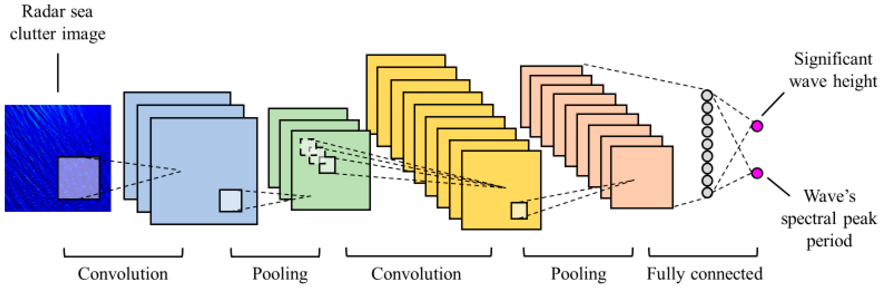
The CNN technique is an important branch of neural networks. It is a feed-forward neural network usually used to solve problems about images. The implementation process of the CNN model is shown in Figure 1. The network architecture of the CNN model mainly consists of the following key elements:

(a) The input layer—Reading images and passing data.

(b) The convolutional layers—Convolutional layers can extract the characteristics of images by convolution. They are the core of CNN. The characteristics of images can be made more prominent through the process of convolution.

(c) Activation function—The use of an activation function is to add nonlinear items so that the networks can effectively deal with nonlinear problems.

(d) Pooling layers—Characteristics output by convolutional layers is large. Pooling layers are used to cut down this number and highlight the main characteristics, which reduces computation.

(e) Fully connected layers—Fully connected layers play the role of finishing classification or regression and outputting the final results. Characteristics of images extracted by pooling convolutional layers are gathered and calculated in fully connected layers.

In fact, there are several methods for extracting geometric features and dissimilarity of remotely sensed imagery [22]. In CNN models, the geometric features and dissimilarity of synthetic radar images are extracted by the convolutional and pooling layers. In short, CNN can be regarded as an input–output mapping, where x represents the input image and y represents the output. The y can be a class, or a numerical value. The f represents the whole network, which is trained by many image data to make the outputs close to actual values. The process of training can be similarly understood as a “function fitting” process.

3.2. Inversion Models of Wave Parameters Based on CNN

Several kinds of network architecture have been proposed, such as AlexNet, GoogLeNet, VGGNet and ResNet. The differences among them mainly lie in the depth of the network and the setting of convolutional layers. In this paper, we chose AlexNet and VGGNet as basic structures to build inversion models under the Tensorflow framework. AlexNet includes five convolutional layers and three fully connected layers, and there are three pooling layers following the three convolutional layers. The ReLU is as the activation function, which is the same as AlexNet. VGGNet includes five convolutional parts and three fully connected layers, although there are several convolutional layers in each convolutional part. Thus, there are 13 or 16 convolutional layers and three fully connected layers in total. Further, to adapt to this two-parameter regression problem, input layers were modified to receive images in RGB and the size of images was 256 × 256 pixels. Output layers and their activation function were also modified to output two target parameters that have continuous values.

Besides network structure, the quality and quantity of the image data are also key factors in building the models. As for the parameter settings of the data set, we will introduce this in detail in Section 5.

4. Numerical Simulation of Radar Sea Clutter Images

In this paper, a number of radar sea clutter images were generated by a numerical simulation program to build the testing and training data sets required by the methods described in Section 2 and Section 3.

4.1. Imaging Principle of X-Band Marine Radar

X-band maritime radar is an active microwave imaging radar with high resolution, which transmits electromagnetic waves to the observed sea surface and receives the backscattered echo signals to realize the observation of sea waves.

The process of X-band radar receiving echo signals can be explained by the Bragg model and two-scale model [3,23]. Moreover, the process involves modulation effects, mainly including hydrodynamic modulation, tilt modulation and shadowing modulation [4,5]. In this section, our numerical simulation program was based on the Bragg model and two-scale model, and involves tilt modulation and shadowing modulation at the same time. Background noise was not considered.

4.1.1. Bragg Model

Bragg scattering is a phenomenon of superposition and interference of backscattered signals. When the wavelength of a sea wave satisfies the condition:

$${\lambda }_s=\frac{n{\lambda }_r\cos \varphi }{2\sin \theta },$$

(10)

then radar echo signals reflected by each wave surface have superposition in the same phase. In Equation (10), ${\lambda }_s$ is the wavelength of the sea surface wave, ${\lambda }_r$ is the wavelength of the radar signal, $\theta$ is the incident angle of radar signal, $\varphi$ is the angle between the direction of the sea wave propagation and the direction of radar signal, and n is a natural number greater than 0.

4.1.2. Two-Scale Model

In two-scale model theory, it is assumed that the sea surface is composed of two scales of waves; microscale waves are superimposed on the long waves. Due to the modulation effect of the tilted wavefront on the microscale wave, the long wave changes the local incident angle of the radar, which affects the backscattering cross section, and finally affects the backscattering signal.

In the calculation, the local scattering cross section in a small area was calculated first, and then the probability density function of the long wave surface slope was used to integrate the whole area. The local scattering cross section is given by:

$${\sigma }^0({\theta }_i)=16\pi k_R^4{\cos }^4{\theta }_i{\left|g({\theta }_i)\right|}^2\psi \prime ,$$

(11)

where the g is the polarization function, $\psi \prime$ is the microscale spectrum and ${\theta }_i$ is the local incident angle,

$${\theta }_i=\arccos \left[\cos \left(\theta +{\delta }_1\right)\cos {\delta }_2\right],$$

(12)

where ${\delta }_1$ is the angle that the local scattering unit normal deviates from the vertical line in the incident plane caused by long wave, and ${\delta }_2$ is the angle of the normal deviating from the vertical line in a plane perpendicular to the incident plane.

Therefore, the backscattering cross section of each little square can be calculated as

$${\sigma }_{PP}^0(\theta )={\displaystyle {\int }_{-\infty }^{\infty }d\left(\tan {\delta }_1\right)}{\displaystyle {\int }_{-\infty }^{\infty }d\left(\tan {\delta }_2\right)}{\sigma }_{PP}^0({\theta }_i)p(\tan {\delta }_1,\tan {\delta }_2),$$

(13)

where $p(\tan {\delta }_1,\tan {\delta }_2)$ is the joint probability density function of the long wave slope.

4.1.3. Tilt Modulation

The Bragg scattering of radar signal to the microamplitude wave is affected by the existence of the long wave. In particular, the angle of the long wave surface changes the normal direction of the backscattering surface, leading to a change of the local incident angle and a change of the backscattering cross section.

4.1.4. Shadowing Modulation

When the incident angle of the radar signal is large and almost parallel to the sea level, then due to the fluctuation of the sea surface, the higher wave will block the sea surface behind it, resulting in a “blind area” that the radar incident signal cannot illuminate. This blind area produces almost no backscattered echo signal.

4.2. Numerical Simulation of Radar Images Data

We developed a numerical program to simulate radar sea clutter images under different sea states based on the above principle. With this program, we could, according to our needs, set the significant wave height and the wave’s spectral peak period of the sea area shown in the radar image. The wave spectrum we chose was the ITTC (International Towing Tank Conference) two-parameter wave spectrum. The model of the ITTC two-parameter wave spectrum is:

$$S(\omega )=\frac{173H_S{}^2}{T_S{}^4{\omega }^5}\exp \left(-\frac{691}{T_S{}^4{\omega }^4}\right),$$

(14)

where H_S is the significant wave height and T_S is the wave’s spectral peak period.

The relation of wave number, wave direction and corresponding wave height is shown in Figure 2.

The left part of Figure 3 shows one synthetic radar image in which the significant wave height H_S is 4 meters and the wave’s spectral peak period T_S is 8.5 seconds. The radius of sea area shown in the image is 3 kilometers. The spatial resolution is 2 × 2 m, and the temporal resolution is 3 seconds.

Figure 4 shows the spatial distributions of water elevation and echo intensity along a radius (Y = 0 m, 300 m < X < 3000 m) of the synthetic image.

Since the size of simulated image was large, we just cut out a square area of 256 × 256 pixels in the image to build training and testing data sets so as to reduce the computational load. Figure 4 also shows the cropping process of the original radar image.

5. Results

5.1. Definitions of the Accuracy Measures

In this paper, accuracy measures including the relative error (RE), mean relative error (MRE), absolute error (AE) and root mean squared error (RMSE) (Equations (15), (16), (17) and (18), respectively), were used to evaluate the performance of both the spectral analysis method and the CNN-based method on wave parameter inversion:

$$\mathrm{RE}=\frac{\left|X_I-X_A\right|}{X_A}\times 100\%,$$

(15)

$$\mathrm{MRE}=\frac{1}{N}{\displaystyle \sum _{i=1}^N\left(\frac{\left|X_I{}^i-X_A{}^i\right|}{X_A{}^i}\times 100\%\right)},$$

(16)

$$\mathrm{AE}=\left|X_I-X_A\right|,$$

(17)

$$\mathrm{RMSE}=\sqrt{{\displaystyle \sum _{i=1}^N{(X_I{}^i-X_A{}^i)}^2}/N},$$

(18)

where $X_I$ is the inversed value of H_S or T_S by the above two methods, while $X_A$ is the actual value and N is the number of samples tested.

5.2. Comparisons of the CNN-Based and Spectral Analysis Methods

Radar sea clutter image sequences under 15 different sea states were generated by the numerical program introduced in Section 4. Each sequence included 16 images continuous in time. The H_S and T_S of these images were set as shown in

Table 1. Parameter settings for the test image sequences.

Sequence Number	HS (m)	TS (s)
1	0.5	6.50
2	1.0	6.79
3	1.5	7.07
4	2.0	7.36
5	2.5	7.64
6	3.0	7.93
7	3.5	8.21
8	4.0	8.50
9	4.5	8.79
10	5.0	9.07
11	5.5	9.36
12	6.0	9.64
13	6.5	9.93
14	7.0	10.21
15	7.5	10.50

. These images were used to test the conventional spectral analysis method.

In the CNN-based method, there needs to be a large number of training data to train the CNN-based models. We used the numerical program to generate 2801 radar images. The H_S of these radar images ranged from 0.5 to 7.5 m, and one image was generated every 0.0025 m. Correspondingly, the T_S ranged from 6.5 to 10.5 s, and was linearly distributed in this range, corresponding to the H_S one-by-one. That is:

$$T_S=4\times \frac{H_S-0.5}{7}+6.5\hspace{1em}\hspace{1em}(\mathrm{s}).$$

(19)

Actually, there was not such a relation between T_S and H_S. We set up this relationship just to make it easier to generate images.

After being cropped in the way introduced in Section 4, 2403 of the 2801 images were used to build the training data set, and 398 of the 2801 were used for validation training. After training, the two CNN-based models, AlexNet-based and VGGNet-based, were tested by test images that were selected from the testing data set of the conventional spectral analysis method. Fifteen test samples were taken from the 15 image sequences, respectively. Using the same test samples to test these two different methods provided more convincing results.

The inversion results of the two methods are shown in

Table 2. Inversion results of the wave’s spectral peak period (T_S).

Sample Number	Actual Value (s)	Spectral Analysis Method		AlexNet-Based Model		VGGNet-Based Model
		Inversed Value (s)	RE 1	Inversed Value (s)	RE 1	Inversed Value (s)	RE 1
1	6.50	8.59	32.15%	6.49	0.15%	6.52	0.35%
2	6.79	8.59	26.58%	6.78	0.02%	6.75	0.46%
3	7.07	9.45	33.61%	7.12	0.71%	7.01	0.85%
4	7.36	6.75	8.27%	7.43	1.01%	7.32	0.55%
5	7.64	5.91	22.74%	7.62	0.28%	7.58	0.86%
6	7.93	9.45	19.17%	7.89	0.50%	7.79	1.74%
7	8.21	9.73	18.48%	8.19	0.29%	7.81	4.88%
8	8.50	9.45	11.16%	8.47	0.35%	8.44	0.73%
9	8.79	8.59	2.23%	8.84	0.62%	8.66	1.47%
10	9.07	9.45	4.16%	9.34	2.98%	8.90	1.92%
11	9.36	7.87	15.85%	9.66	3.26%	9.40	0.47%
12	9.64	10.54	9.33%	10.09	4.66%	9.65	0.11%
13	9.93	9.45	4.84%	9.87	0.61%	10.04	1.11%
14	10.21	9.73	4.72%	10.05	1.57%	9.71	4.98%
15	10.50	10.54	0.40%	10.25	2.39%	10.08	3.96%

¹ RE is the Relative Error.

and

Table 3. Inversion results of significant wave height (H_S).

Sample Number	Actual Value (m)	Spectral Analysis Method		AlexNet-Based Model		VGGNet-Based Model
		Inversed Value (m)	RE	Inversed Value (m)	RE	Inversed Value (m)	RE
1	0.5	0.62	24.75%	0.58	16.14%	0.58	15.22%
2	1.0	1.22	21.77%	1.03	2.52%	1.05	5.34%
3	1.5	1.95	30.31%	1.60	6.99%	1.59	5.70%
4	2.0	1.75	12.71%	2.10	4.78%	2.06	2.80%
5	2.5	1.84	26.58%	2.57	2.74%	2.64	5.80%
6	3.0	2.24	25.23%	3.04	1.21%	3.13	4.49%
7	3.5	4.12	17.61%	3.53	0.91%	3.21	8.30%
8	4.0	3.83	4.33%	3.91	2.30%	4.10	2.52%
9	4.5	4.09	9.04%	4.58	1.78%	4.43	1.49%
10	5.0	6.55	31.03%	5.37	7.47%	4.90	2.03%
11	5.5	4.09	25.72%	5.96	8.41%	5.70	3.56%
12	6.0	6.84	13.93%	6.70	11.68%	6.12	1.96%
13	6.5	8.08	24.37%	6.68	2.73%	6.88	5.91%
14	7.0	5.65	19.33%	6.71	4.12%	6.22	11.17%
15	7.5	5.83	22.22%	7.18	4.26%	7.04	6.07%

.

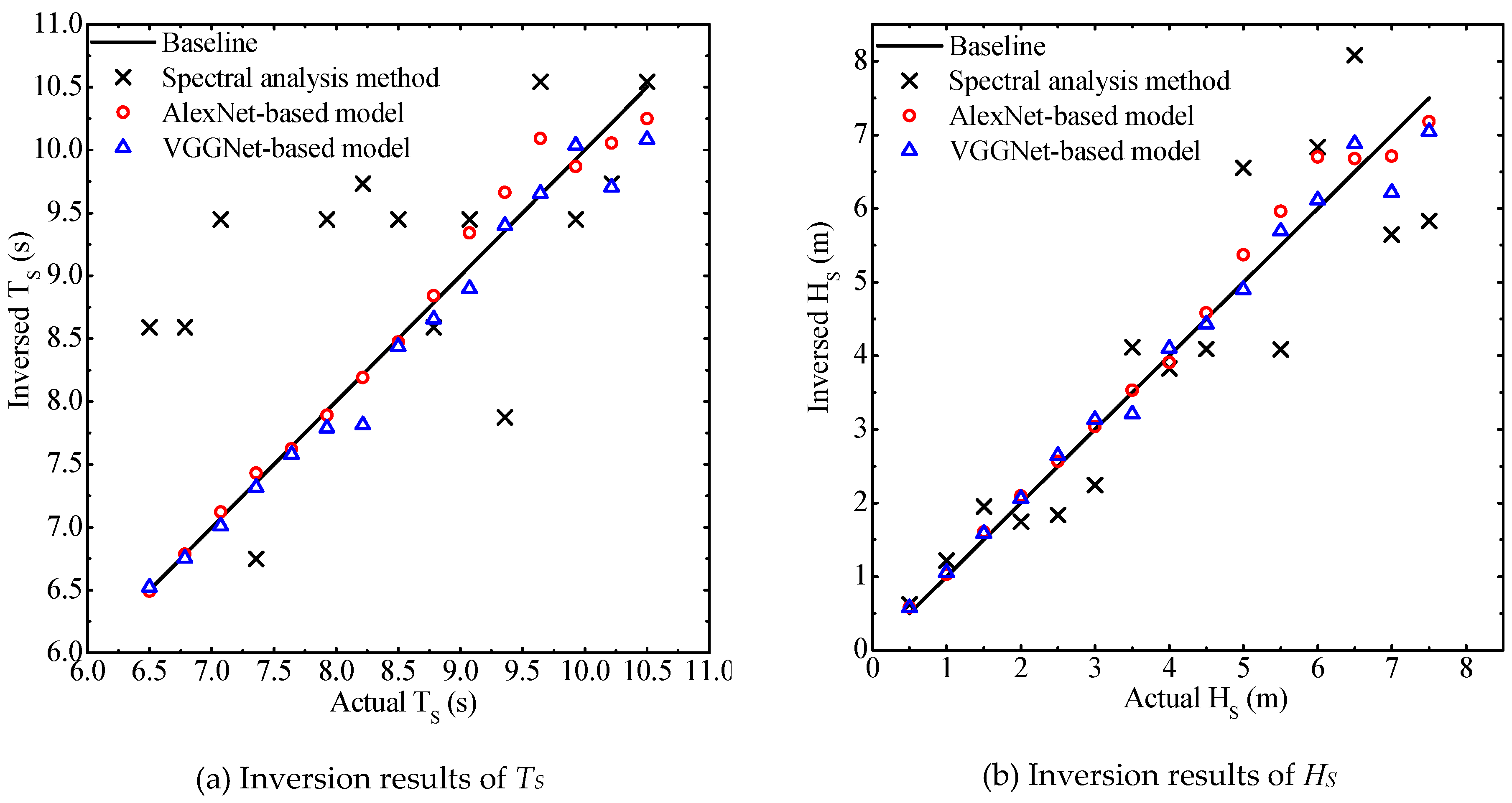
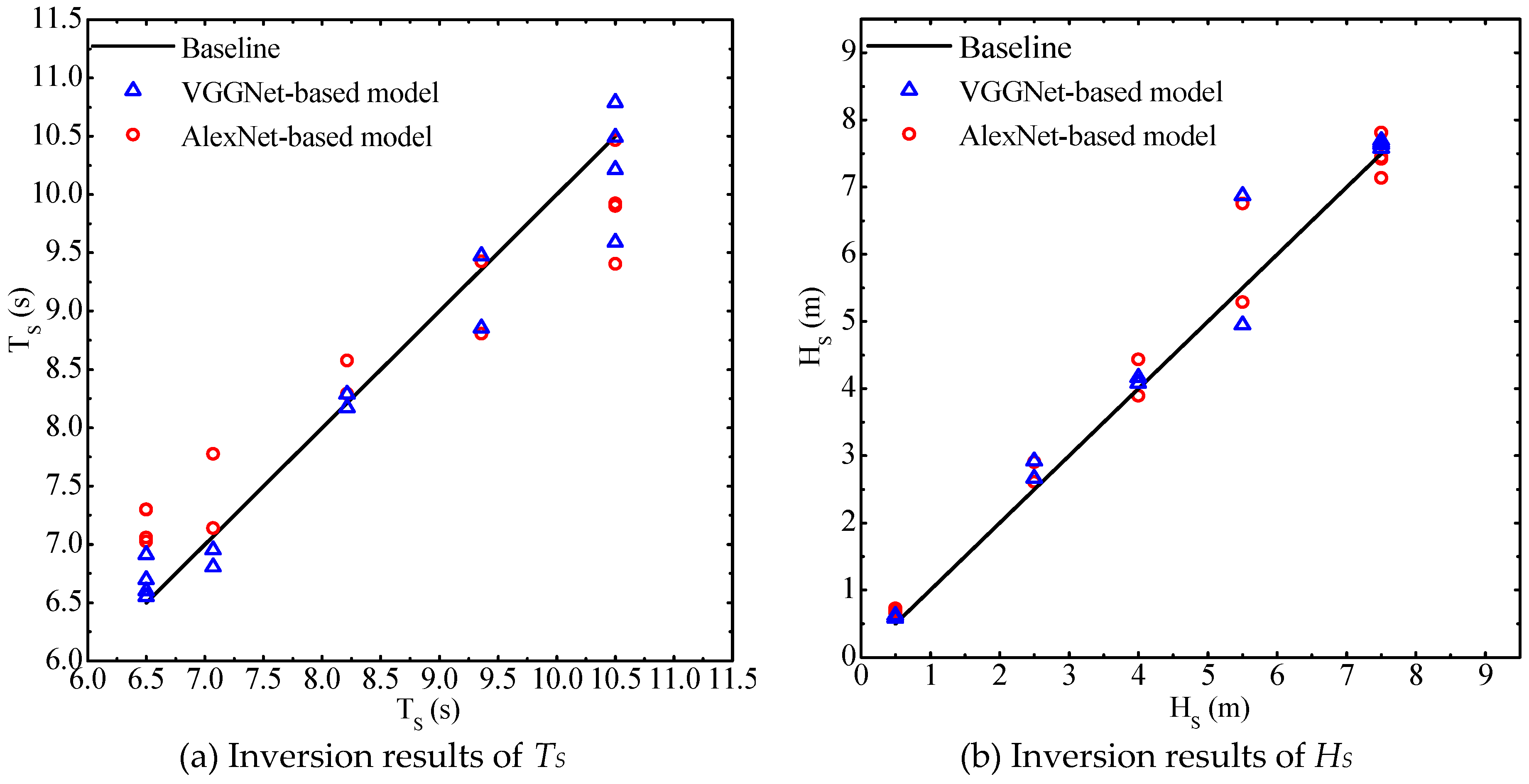
In Figure 5, we can see intuitively the difference between the results of the above methods. The distance between inversion points and the baseline can indicate the inversion errors (Figure 5a,b).

The results’ statistical characteristics of the two methods are shown in

Table 4. Statistical characteristics of results inversed by the spectral analysis and CNN-based methods.

		Mean Relative Error	Root Mean Squared Error
Inversion results of TS	Spectral analysis method	14.25%	1.31 s
	AlexNet-based model	1.29%	0.18 s
	VGGNet-based model	1.63%	0.21 s
Inversion results of HS	Spectral analysis method	20.59%	0.97 m
	AlexNet-based model	5.20%	0.27 m
	VGGNet-based model	5.49%	0.28 m

.

5.3. Training Dependence of the CNN-Based Inversion Models

We developed numerical experiments to study the dependence of CNN-based inversion models on the training data set for two aspects, the parameter setting range of the training images and the position where the training images are cut out from the original radar image.

5.3.1. Dependence of CNN-Based Inversion Models on the Pparameter Setting Range of the Training Images

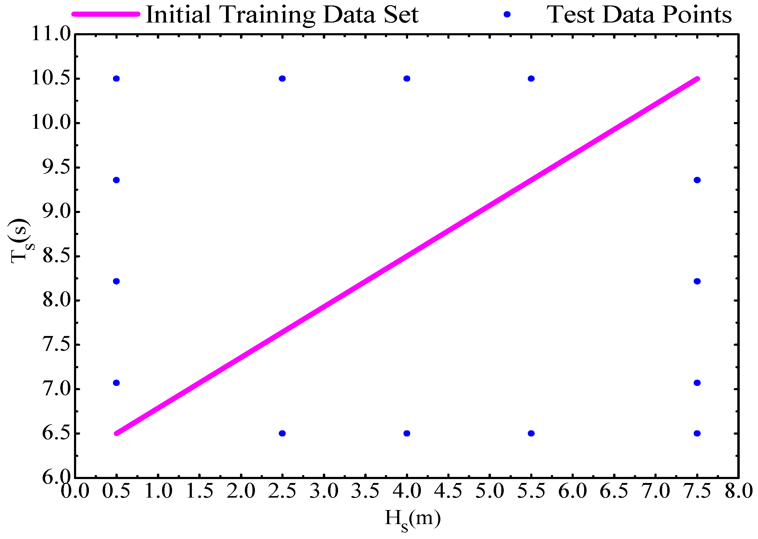
The relationship between the T_S and H_S of images in the training set for CNN-based inversion models introduced in Section 5.2 are represented by the line in Figure 6.

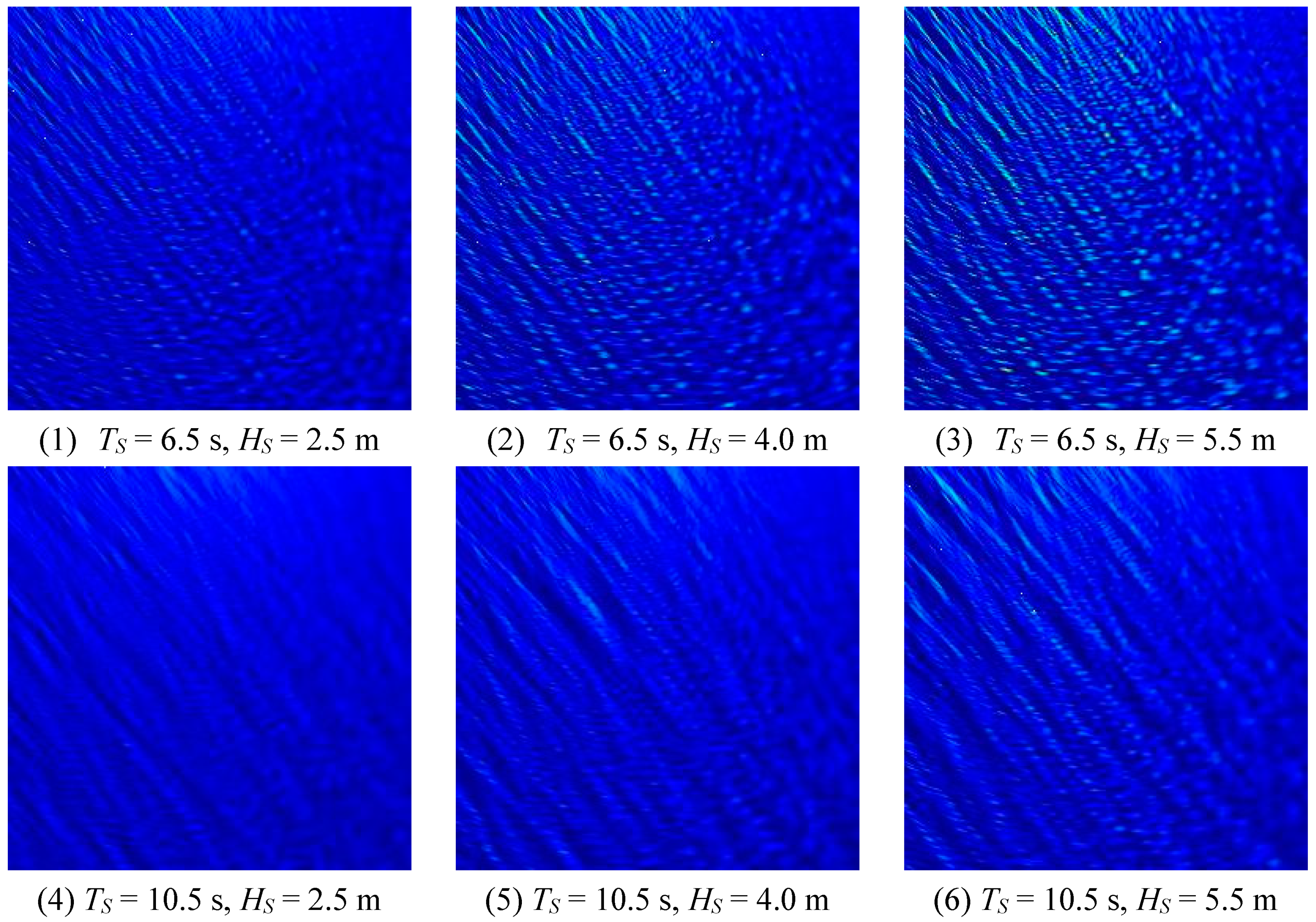
However, the T_S and H_S do not correspond one-to-one to each other in the actual ocean. The relationship shown by the line in Figure 6 is only for the maximum probabilities. We simulated some radar images beyond the coverage shown by this line according to the relationship between the wave’s spectral peak period and the significant wave height [24], to test the CNN models trained by the initial training set. The parameters of the test samples are shown in

Table 5. Parameter settings for the test samples.

Sample Number	HS (m)	TS (s)
1	0.5	7.07
2	0.5	8.21
3	0.5	9.36
4	0.5	10.50
5	2.5	6.50
6	2.5	10.50
7	4.0	6.50
8	4.0	10.50
9	5.5	6.50
10	5.5	10.50
11	7.5	6.500
12	7.5	7.071
13	7.5	8.214
14	7.5	9.357

and the distribution of the test samples is shown as the blue points in Figure 6. Some of the test sample images are shown in Figure 7.

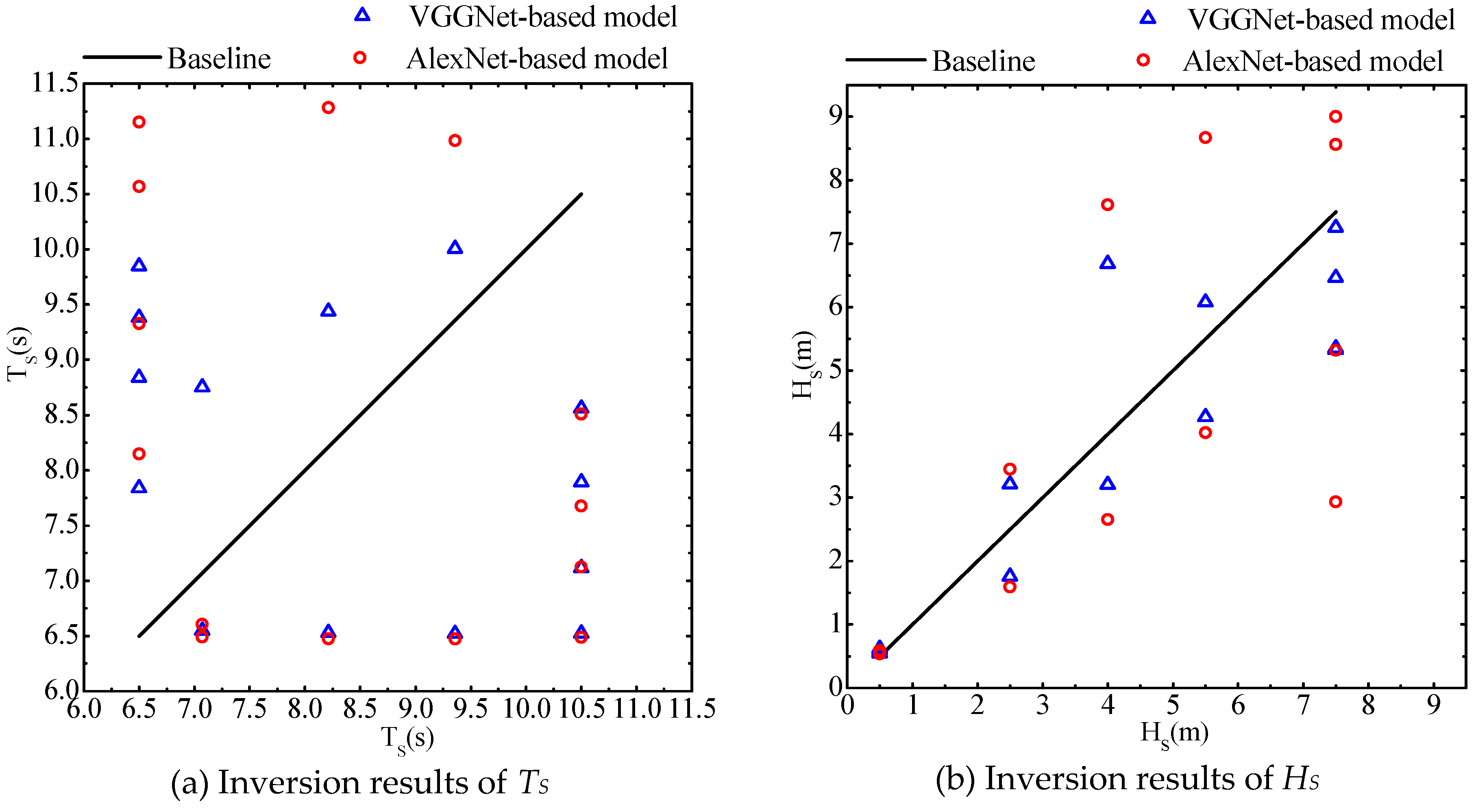
The results of the 14 test samples inversed by the CNN-based models and trained by the initial training data set are shown in Figure 8.

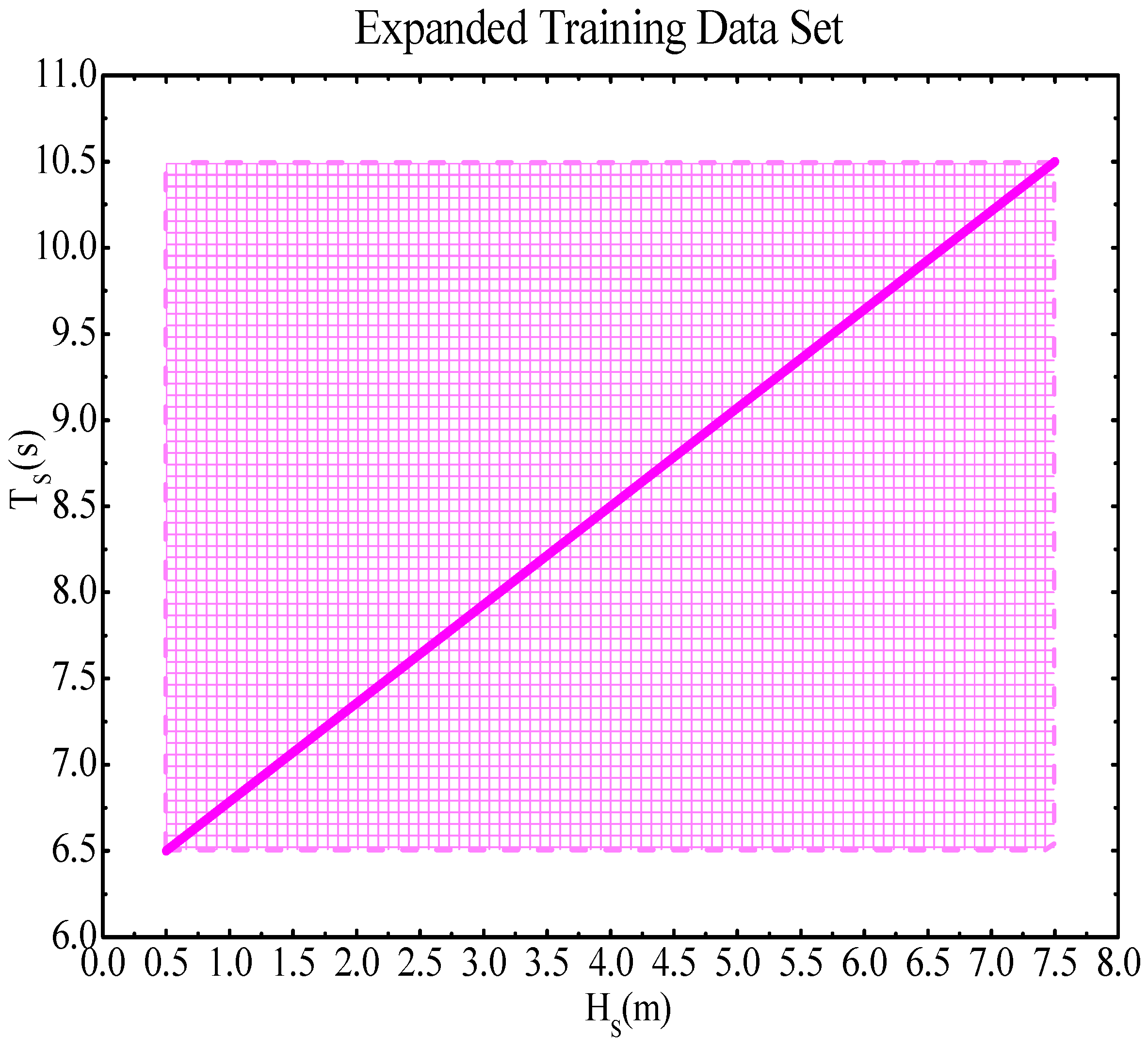
We can see that there were obvious errors because of the difference between the test samples and the training data. To address this problem, we expanded the training data set as shown in Figure 9; one radar image was generated every 0.008 s in T_S at the same H_S, and one radar image was generated every 0.014 m in H_S at the same T_S.

We trained the CNN-based models with the expanded training data set. Afterward, the two models were used to inverse H_S and T_S of the 14 test samples. Results are shown in Figure 10.

From Figure 10, we can see that after being trained by the expanded training set, CNN-based models’ inversion accuracy increased greatly.

Table 6. Inversion MRE (mean relative error) of CNN-based models trained by the initial and expanded training sets.

	AlexNet-Based Model		VGGNet-Based Model
	TS	HS	TS	HS
Trained by initial training set	31.49%	32.46%	26.40%	22.51%
Trained by expanded training set	6.14%	16.24%	2.82%	10.73%

gives the errors in detail.

According to Table 6, we see that the MRE of T_S and H_S inversed by the two CNN-based models trained by the initial training data set were 31.49% and 26.40%, 32.46% and 22.51%, respectively. By comparison, the MRE of T_S and H_S inversed by CNN-based models trained by the expanded training data set were 6.14% and 2.82%, 16.24% and 10.73%, respectively.

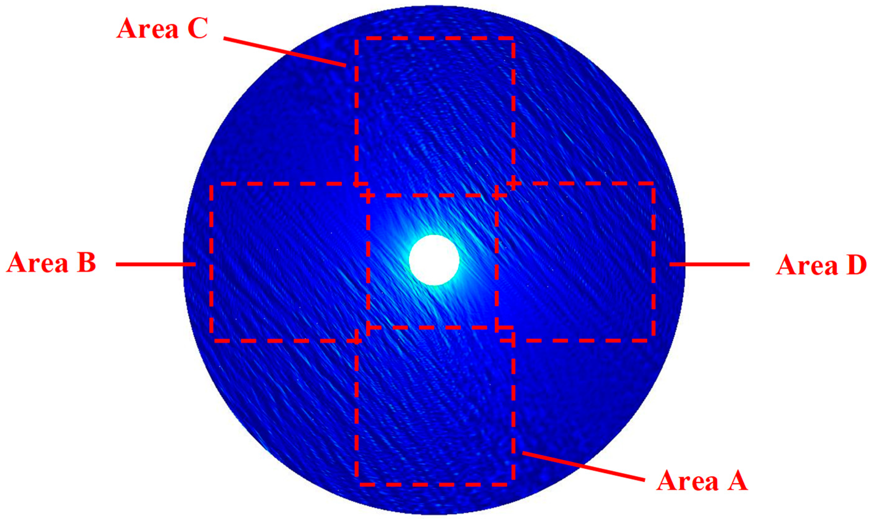
5.3.2. Dependence of CNN-Based Inversion Models on the Cropping Position of Images

In Section 4.2, we introduced a method of cropping the original image to reduce the computation effort. However, in the original radar image the characteristics information contained in various positions may be different. The training images cut out from the original radar images may only contain local information of the wave. In this section we describe a numerical experiment developed to study whether CNN-based models trained by local area images could correctly inverse the information of other area images that were not involved in training.

To begin, we named the area cut out in Section 4.2 Area A. Then, three images with the same size were cut out from the other three areas: B, C and D in the original image, as shown in Figure 11.

The images of Area B, Area C and Area D were used for training, and the images of Area A were used for testing to validate whether CNN-based models could extract global characteristics information from local area images. Test results of two CNN-based models are shown in Figure 12 and

Table 7. Inversion errors of wave’s spectral peak period (T_S) and significant wave height (H_S) by CNN-based models.

	Errors	HS		TS
CNN-Based Model		MRE	RMSE	MRE	RMSE
AlexNet-based model		64.18%	1.25 m	7.46%	0.64 s
VGGNet-based model		7.54%	0.39 m	1.61%	0.20 s

.

5.4. Effects of Wave Parameters on Inversion Accuracy of the CNN-Based Models

CNN-based inversion models showed different inversion accuracy for T_S and H_S. In this section, we explore the influence of changes of two inversion target parameters on the inversion accuracy of CNN-based models. In order to eliminate the influence of training set on the results, the CNN models used in this section were trained by the expanded training data set.

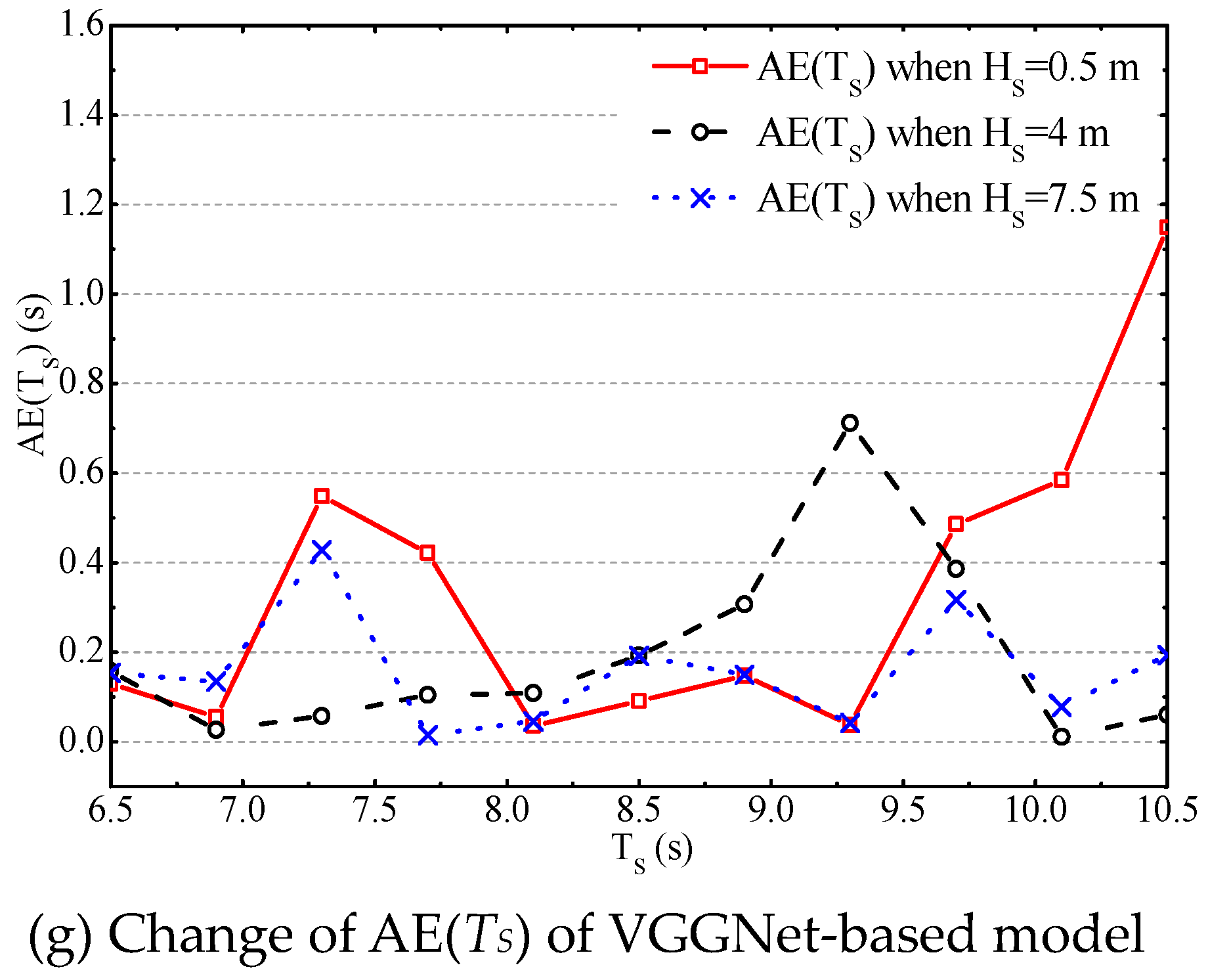
We first considered the influence of the change of T_S on the CNN-based models with the same H_S. In order to avoid the influence of particularity of selected H_S on the results, we used the numerical simulation program to generate radar images under three H_S: 0.5, 4 and 7.5 m. Eleven images with different T_S were generated under each H_S. T_S was set to 6.5, 6.9, 7.3, 7.7, 8.1, 8.5, 8.9, 9.3, 9.7, 10.1 and 10.5s, respectively. After being cropped, the 33 images were used as input to the CNN-based models as test samples.

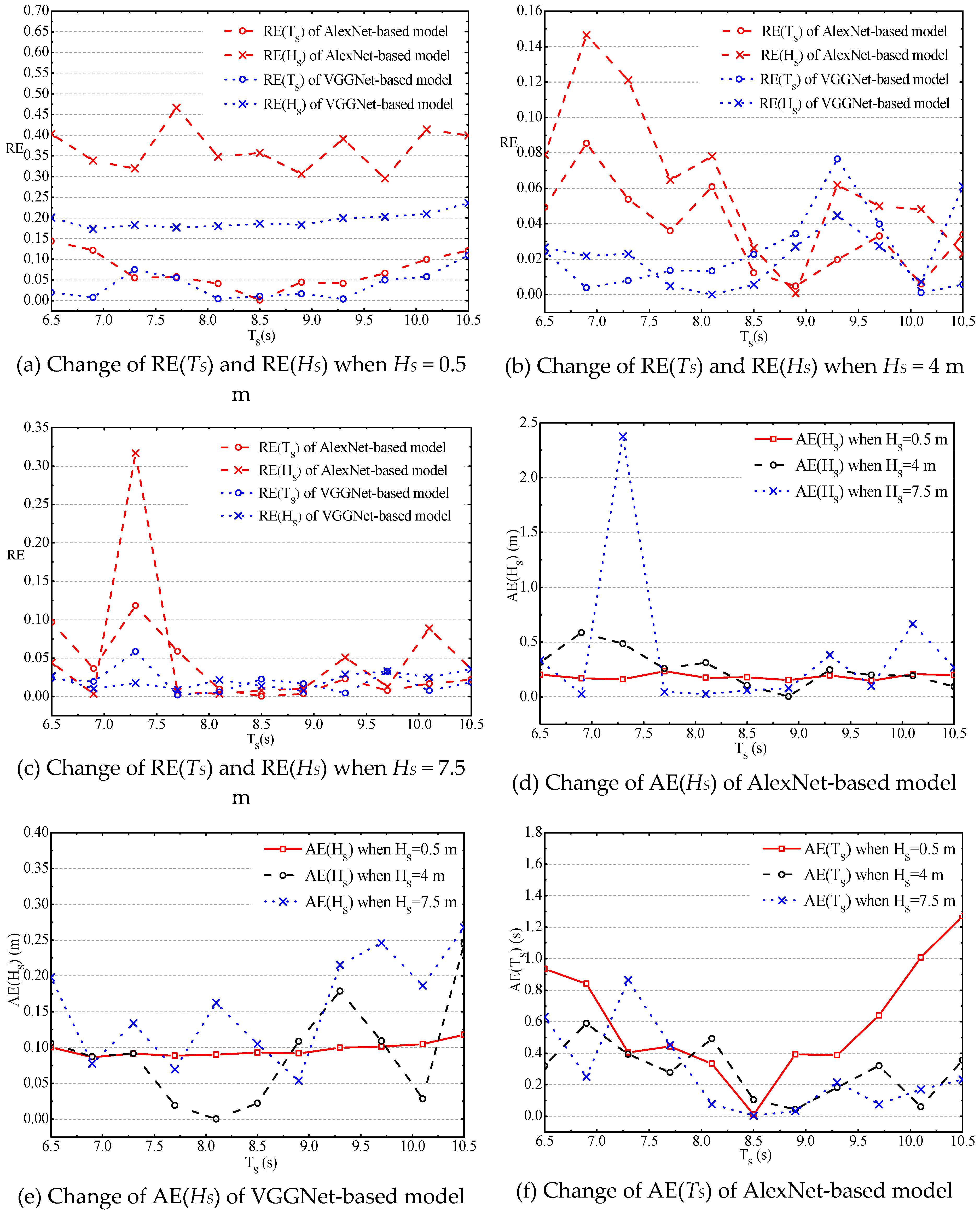
Figure 13 shows the change of RE and AE. For example, Figure 13a shows the changing trend of RE(T_S) and RE(H_S) with changing T_S when H_S = 0.5 m. The red dash lines with cross and circle symbols represent the RE(T_S) and RE(H_S) of the AlexNet-based model, while the blue dot lines with cross and circle symbols represent the RE(T_S) and RE(H_S) of the VGGNet-based model. It is the same in Figure 13b,c except that they were under different H_S. According to Figure 13a–c, regardless of red lines or blue lines, there was no uniform regularity of these changes. The changes of RE for H_S and T_S were generally irregular when T_S changed and H_S was constant.

Figure 13d,e shows the changes of AE(H_S) when applying the AlexNet-based and VGGNet-based models. In this figure, the red lines with squares represent the AE(H_S) when H_S = 0.5 m, while the black lines with circles represent AE(H_S) when H_S = 4 m, and the blue lines with crosses represent AE(H_S) when H_S = 7.5 m. Analogously, Figure 13f,g shows the changes of AE(T_S). The changing trend of AE was also generally irregular.

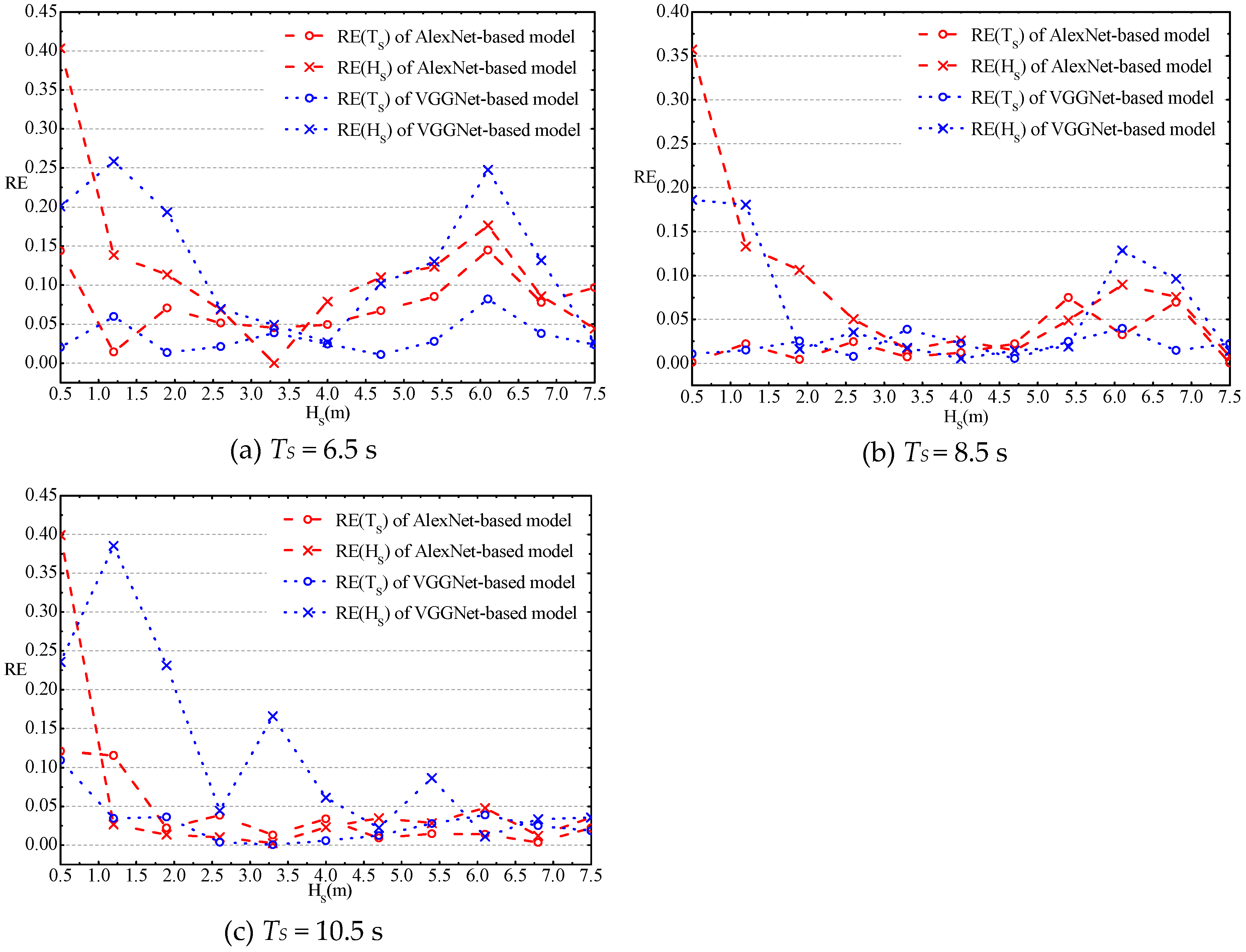
Next, T_S remained constant and the influence of the change of H_S on the CNN-based models was studied. T_S was set to 6.5, 8.5 and 10.5 s, and 11 images with different H_S were generated under each T_S. H_S was 0.5, 1.2, 1.9, 2.6, 3.3, 4, 4.7, 5.4, 6.1, 6.8 and 7.5m, respectively. These images were input into the CNN-based inversion models after being cropped. The changes of inversion RE are shown in Figure 14.

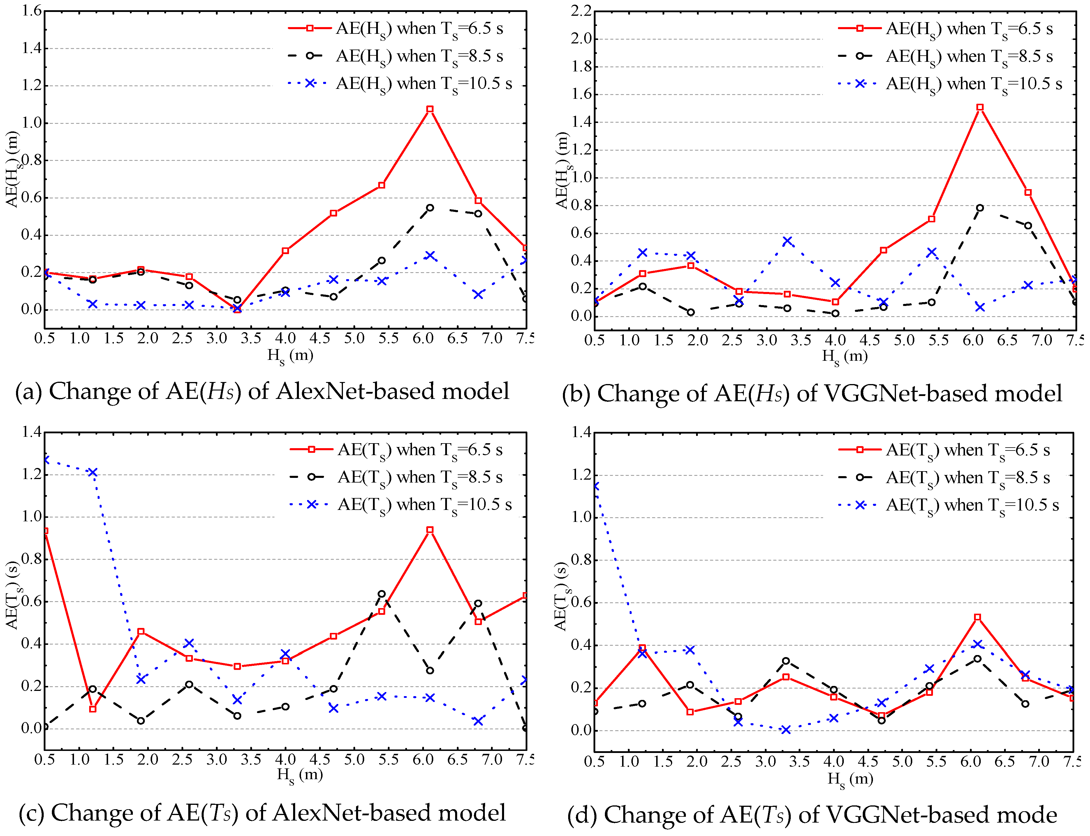
In Figure 14, blue and red lines with circles represent RE(T_S) of the two CNN-based models. Generally, these lines change irregularly. For the inversion RE(H_S), however, which are represented by the red and blue lines with crosses, it decreased with the increase of H_S. The RE(H_S) was large when the value of H_S was small. To research this problem further, we show the change of AE in Figure 15.

According to Figure 15, the change of AE(H_S) did not have the same regularity with RE(H_S). It was generally irregular.

6. Discussion

In Section 5.2, the inversion accuracy of the CNN-based method was compared with the accuracy of the conventional spectral analysis method using the same data set. From Figure 5, we can see that, entirely, the results of H_S and T_S inversed by the CNN-based models were in good agreement with actual values. According to Table 4, the MRE of T_S inversed by the two CNN-based models were 1.29% and 1.63%, and RMSE were 0.18 s and 0.21 s. At the same time, the MRE of H_S were 5.20% and 5.49%, respectively, the RMSE were 0.27 m and 0.28 m. These errors are acceptable. So, we can say that the CNN-based method is a feasible way to inverse wave parameters from our synthetic radar images. In comparison, as for the spectral analysis method, MRE of T_S and H_S were 14.25% and 20.59%, while RMSE were 1.31 s and 0.97 m, respectively. Both CNN-based models had higher accuracy than the spectral analysis method in this inversion problem. For these test samples, the errors of the conventional method, regardless of relative or absolute errors, were greater than those of the CNN-based method. It shows there are advantages of the CNN-based method when compared to the conventional spectral analysis method, to some extent.

In Section 5.3, the dependence of CNN-based inversion models on the training data set was studied in two aspects: the range of parameter settings for the training images and the position where the training images are cut out from the original radar image. In the first aspect, according to the results, it is obvious that the accuracy of the CNN-based model trained by the expanded training data set was much higher than that of the CNN model trained by the initial training data set. The initial training data set did not cover the test samples, while the expanded training data set covered them (but they were not a part of expanded training data). This phenomenon shows that the CNN method is ineffective in dealing with data not covered by the training set. It also reveals that CNN is a data-driven method. Thus, the quantity and quality of training set data are the key factors affecting the performance of the CNN-based models. In the second aspect, it is clear that inversion errors of AlexNet-based model were large. Especially, the MRE of H_S reached 64.18%. That is, the AlexNet-based model could not inverse H_S and T_S of Area A images correctly according to the characteristics information which it learned from the images of Area B, C and D. Therefore, we conclude that the AlexNet-based model was unable to learn the global characteristics information from local images. In contrast, the VGGNet-based model had high accuracy, and its inversion errors were all within an acceptable range. Therefore, we believe that the VGGNet-based model extracted information about H_S and T_S from the images of Area B, C and D and applied it to the inverse parameters of the Area A images. Furthermore, the VGGNet-based model could obtain the global characteristics information from local images. As for the reason for the above phenomenon, we infer that because the architecture of VGGNet is deeper, it is more effective than AlexNet for complex characteristics information. Hence, the VGGNet-based model had better performance in this problem. The more detailed reasons will be studied in our follow-up work.

Finally, in Section 5.4, the influence of changes for two inversion target parameters on inversion accuracy of CNN-based models was studied. When T_S changed and H_S was constant, the changes of RE(T_S), AE(T_S), RE(H_S) and AE(H_S) were all generally irregular. When H_S changed and T_S was constant, it appeared that the RE(H_S) was larger when the value of H_S was smaller. After the changes of AE(H_S) were drawn, we concluded that the reason why RE(H_S) decreases with increasing of H_S was the definition of relative error. According to the definition of RE, when the AE(H_S) is the same, if the value of H_S is smaller, then RE(H_S) will be larger. Therefore, in summary, the changes of T_S and H_S did not obviously affect the inversion AE of the CNN-based models, although the RE(H_S) was affected by the value of H_S. The RE(H_S) was larger when H_S was smaller.

7. Conclusions

Conventional wave inversion methods are limited by assumptions involved in the calibration process. It is challenging to further improve wave inversion accuracy by using these methods. Inspired by the capability of CNN techniques in handling image problems, a machine learning inversion method based on CNN was proposed. Comparison studies, training strategy and training data dependency were investigated. Some concluding remarks are summarized as follows.

The inversed results of both spectral peak periods and significant wave heights by the AlexNet-based and VGGNet-based models were highly correlated to the targets. The mean relative error was within an acceptable range. It was demonstrated that CNN models could effectively extract the characteristic periods and wave heights from radar images. It also verified the feasibility of using CNN to extract information from radar sea clutter images. Furthermore, compared to the conventional spectral analysis method, the CNN-based method produced higher accuracy. The method therefore provides a potential way for accurate wave parameter inversion from radar images.

Results of the training data set dependence on CNN-based inversion models show that CNN models only performed well when the test image data had the same wave parameter ranges as the training data set. There were obvious inversion errors if test samples resulted from wave parameters out of the training data range. These results provide the scope of applicability for the CNN models in wave inversion. Comparatively, the VGGNet-based model could obtain the overall wave characteristics of radar images from local cropped pictures, although the AlexNet-based model failed.

Finally, as for the effects of the target wave parameters on the inversion results, it was indicated that the changes of spectral peak period and significant wave height had little effect on inversion accuracy of the CNN-based method.

However, in this paper, the validation of the method was based on a synthetic image data set. The CNN-based models were effective on the synthetic image data set, but further testing is necessary to establish whether the method is suitable for a real radar image data set. Moreover, the CNN-based method is presently unable to inverse the wave direction. These problems will be important parts of our follow-up study.