Understanding Fields by Remote Sensing: Soil Zoning and Property Mapping


1
AgriCircle, Rapperswil-Jona, 8640 St.Gallen, Switzerland
2
Group of Crop Science, Department of Environmental Systems Science, ETH Zurich, 8092 Zurich, Switzerland
3
LUFA Nord-West, Jägerstr. 23 - 27, 26121 Oldenburg, Germany
4
Water Protection and Substance Flows, Department of Agroecology and Environment, Agroscope, Reckenholzstrasse 191, 8046 Zürich, Switzerland
*
Author to whom correspondence should be addressed.
Remote Sens. 2020, 12(7), 1116; https://doi.org/10.3390/rs12071116
Submission received: 27 February 2020
/
Revised: 28 March 2020
/
Accepted: 29 March 2020
/
Published: 1 April 2020
(This article belongs to the Section Remote Sensing in Agriculture and Vegetation)
Abstract
:Precision agriculture aims to optimize field management to increase agronomic yield, reduce environmental impact, and potentially foster soil carbon sequestration. In 2015, the Copernicus mission, with Sentinel-1 and -2, opened a new era by providing freely available high spatial and temporal resolution satellite data. Since then, many studies have been conducted to understand, monitor and improve agricultural systems. This paper presents results from the SolumScire project, focusing on the prediction of the spatial distribution of soil zones and topsoil properties, such as pH, soil organic matter (SOM) and clay content in agricultural fields through random forest algorithms. For this purpose, samples from 120 fields were investigated. The zoning and soil property prediction has an accuracy greater than 90%. This is supported by a high agreement of the derived zones with farmer’s observations. The trained models revealed a prediction accuracy of 94%, 89% and 96% for pH, SOM and clay content, respectively. The obtained models for soil properties can support precision field management, the improvement of soil sampling and fertilization strategies, and eventually the management of soil properties such as SOM.
1. Introduction
Remote sensing plays an increasing role in near real-time soil, crop, and pest management in precision agriculture [1]. The primary purpose of using remote sensing data for precision agriculture is to identify the in-field variability of soil and plant properties and subsequently optimize crop management to maximize crop performance and minimize environmental effects [2]. Hence, precision agriculture needs effective decision support systems to optimize crop production while optimizing the usage of resources.
In early precision agriculture applications, farmers used set markers with GPS coordinates to understand and correct spatial vegetation variability in their fields. The field input applications started to benefit from satellite and unmanned aerial vehicle (UAV) imagery [3,4,5] by the end of the 1990s. Today, remote sensing data from satellites allow gathering spectral and temporal information. Such data help to interpret not only crop vitality (chlorophyll content) [6,7] and productivity (biomass) [8] but also soil properties, including physical (texture) [9], chemical (pH value or nutrient contents) [10], and biological (soil organic carbon) [11] properties.
In current precision agriculture practices, two of the most commonly used data sources are multi-spectral optical (MS) [1] and synthetic aperture radar (SAR) [12] data. The imagery from MS systems provides reflectance information in the visible and infrared part of the light spectrum, which usually ranges between 300 to 2500 nm. They are considered as passive systems and need an additional illumination source, the sun. Therefore, they cannot provide imagery during the night or cloudy conditions. SAR, on the other hand, is an active system that has >1 cm wavelength. By being an active system and due to its high wavelength, SAR can provide data independent of the time of the day and cloud conditions. SAR data carries intensity and phase information of scattered electromagnetic waves. The intensity shows sensitivity towards the physical/texture properties of the scene, while the phase includes information in the third dimension (surface roughness or crop height) via the attenuation of the waves within the scene. In terms of agricultural practices, MS data provides info on crop vitality and soil properties, and with its polarized waves, SAR data provides info on crop morphology and scene topography [13,14,15]. Considering both systems, the combined use of SAR and MS data broadens the extent of precision agriculture applications.
For precision agriculture applications, the monitoring of relevant soil and crop properties is essential. For soil monitoring, moisture content, pH, soil texture, and soil organic matter (SOM) an indicator for soil organic carbon (SOC) are among the most critical soil parameters needed to optimize crop management [2,16,17,18]. For crop monitoring, remote sensing data often delivers information on vegetative density, biomass, yield, growth stage, and canopy health [1,12,14,19]. It is essential to emphasize the link between crop performance and the properties of the underlying soil to be able to investigate the changes in the field.
Understanding the chemical, biological, and physical properties of soils, such as pH, SOM, and texture, is crucial for optimizing field management. Such properties are particularly important for fertilizer application for most nutrients and cropping systems [20,21,22]. In agricultural fields, the stated soil properties often show significant spatial in-field variations in both, soil surface and in the soil profile. Therefore, soil profiling was used to understand these variances for mapping of soils or agricultural productivity potential. Their texture distinguishes the identified soil horizons, i.e., clay, silt and sand content, pH, and SOM [23,24,25], among others. However, soil profiling is very laborious and time-consuming. Today, remote sensing provides spatial guidance in crop performance, such as biomass maps based on spectral indices such as the normalized difference vegetative index (NDVI) [26,27]. Although crop performance and soil properties are tightly related, soil profiling and biomass maps do not always reflect the same heterogeneity in the field [28]. Remote sensing of soil properties can help to overcome this discrepancy and improve decision support for precision agriculture applications allowing a high resolution and in-season identification of regions, where soil shows similar bio-geochemical properties, often referred to as soil zones.
Soil zoning has been an exciting topic in research [26] for its importance in precision agriculture practices [29,30]. Identification of spatial variation of soil properties in the field is particularly significant for understanding crop dynamics and thus are often the base to defining management zones [28,30].
Current soil property mapping campaigns have gained relatively high accuracy for the detection of chemical, physical, and biological soil properties such as pH [10], SOM [11] and clay content [9], respectively. Although these maps are relatively low in spatial and temporal resolution, they are needed for precision crop management. Management zones can be defined as relatively homogeneous sub-units of a field that can be managed with a different, but uniform customized management practice [1], such as soil tillage, sowing density, fertilizer application, crop protection, and other measures.
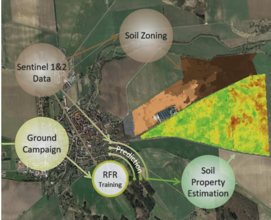
This research investigates the remote detection of soil zones with similar properties that are potentially suitable for precision crop management. The soil zones and their properties are predicted using both MS and SAR data as well as machine learning models. The first part of this research combines MS and SAR data to identify regions of similar properties in fields, group them in zones, and validate zone differences with zone-based soil sampling. The second part focuses on the generated zones and soil properties to predict the soil property distribution through random forest regressor models on the pixel level. The chosen soil properties were soil pH, SOM, and clay content, which are soil properties often used to define management zones or to classify soil properties for agronomic interpretation. The SAR and MS data required for the soil zoning are obtained from the Copernicus satellites via the Google Earth Engine (GEE) platform [31]. This manuscript contributes to precision agriculture as supported by satellite remote sensing. In particular, it delivers unsupervised soil zoning and subsequent zone sampling based soil property prediction enabling improved spatial management of the field inputs.
2. Materials and Data Acquisition
2.1. Satellite Data
2.2. Google Earth Engine
For this research, the S1 and S2 imagery were downloaded using the Google Earth Engine (GEE) Python API. The GEE was established in 2010, aiming to provide an online platform to access, analyze, and visualize up-to-date remote sensing data. Within the GEE platform, S1 images are provided in level-1 Ground Range Detected (GRD) format, which is back-scattering intensity values not having the phase information. S2 images, on the other hand, are downloaded as level-2a surface reflectance values [31].
2.3. Study Areas
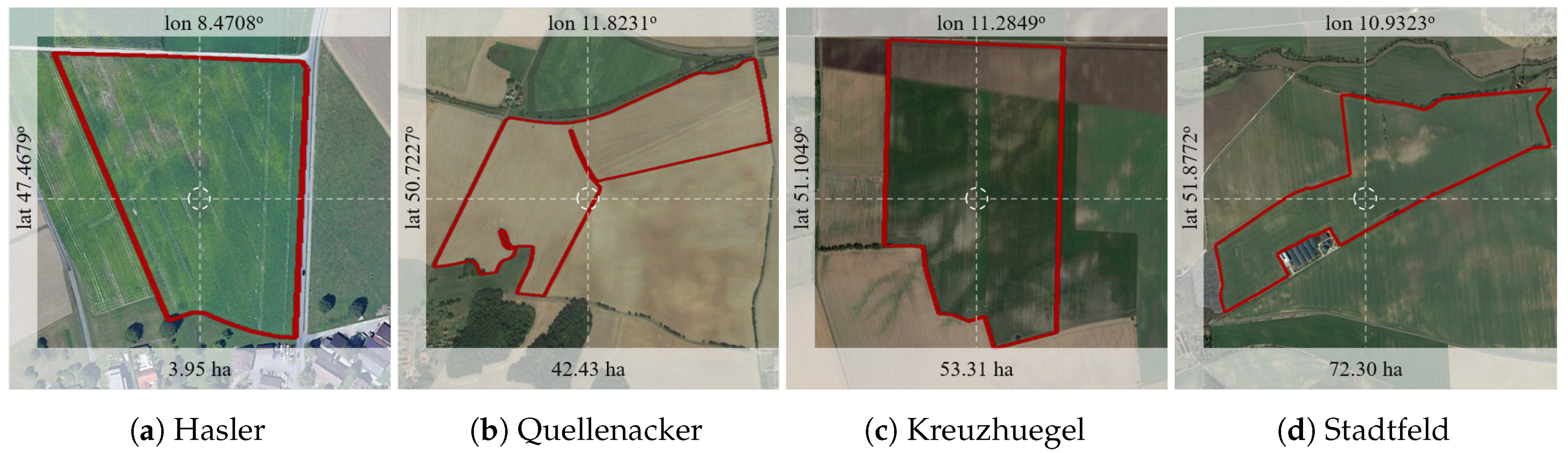
This manuscript evaluates four fields selected from a larger dataset containing a total of 120 fields from Switzerland and Germany. These four fields are managed by local farmers and known to have different soil properties, management practices and sizes. Hasler, Figure 1a, is located in Switzerland and has an area of 3.95 ha. Quellenacker, Kreuzhuegel, and Stadtfeld Figure 1b–d, are located in Germany and have an area of 42.43 ha, 53.31 ha, and 72.30 ha, respectively. All fields were reported to be heterogeneous in their soil characteristics and observed crop performance.
2.4. Soil Sampling and Vegetation Performance
Soil sampling for its properties analyses was conducted by the laboratory of the Chamber of Agriculture of Lower Saxony (LUFA Nord-West) in Germany and by the Swiss Federal Institute of Technology (ETH) Zürich for the Swiss fields. Soils were sampled during two sampling campaigns in 2018 according to the satellite-based soil zoning approach. The first campaign aimed to generate data for training and testing of the soil property prediction model. A minimum of 20 samples was taken from each soil zone with a depth between 25 to 30 cm (according to managed soil depth) from 95 fields in Germany and 25 fields in Switzerland, which sums up to more than 450 distinct zones, meaning soil samples. The fields Hasler, Quellenacker, and Kreuzhuegel were sampled during the first campaign. The mentioned fields lay in a typical arable farming area with heavy soils. The second campaign (only in Germany) aimed to generate an independent validation data set where five independent fields were selected and sampled on precise locations. The locations were identified using the variance of the spectral features to sample them homogeneously. Stadtfeld represents the validation data in this paper. The soil samples were analyzed by LUFA Nord-West and Agroscope laboratories for several soil properties, including clay content, SOM being 1.74x times soil organic carbon (SOC), and pH, which are presented here. Clay content was not measured in the second campaign samples. The soil analysis was done according to reference methods [34]. For monitoring of crop performance, two remote sensing-based vegetation indicator maps are evaluated in the investigated soil zones.
3. Processing and Analysis Methods
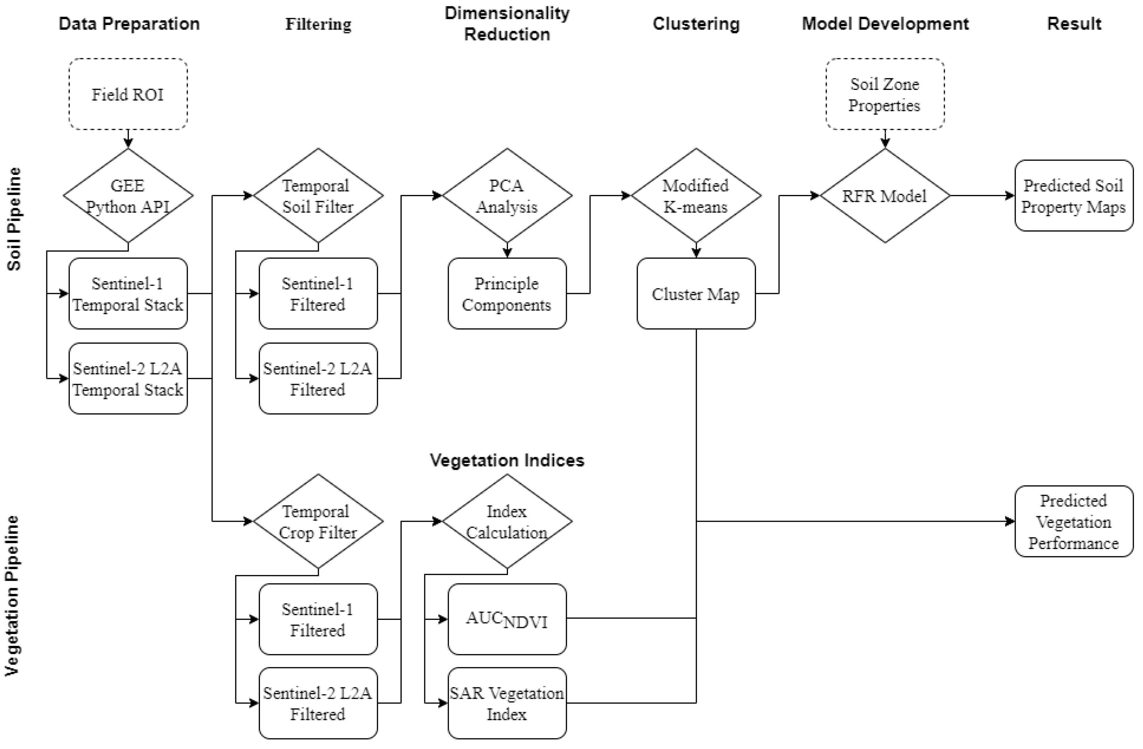
The proposed satellite-based soil zoning approach consists of six sequential steps to be applied to a single field. The developed process chain, shown in Figure 2 as column names, starts with data preparation and continues with data filtering, dimensionality reduction, clustering, and finally, the generation of soil similarity maps. The process chain requires only the geo-referenced field shape from a selected region of interest (ROI) as an input.
3.1. Data Preparation
The current implementation of the proposed soil zoning algorithm works at the field scale and requires the field shape, i.e., ROI, as an input. On the provided ROI, the Python API of the GEE platform was used to collect the available S1 and S2 data between 1 April 2015, and 31 December 2018. S1 data have around 36 degree incidence angle and VV-VH polarizations. The polarization pair of VV-VH was chosen due to its sensitivity to bare-soil and vertically structured vegetation [35]. S2 data comes as a Level-2a product, which corresponds to bottom-of-atmosphere reflectance, filtered before download with its derived cloud band to have clear sky images directly on the GEE servers.
Before filtering, downloaded S1 and S2 data is used to form a four-dimensional image stack. The dimensions of the image stack correspond to image x-size, image y-size, image-bands, and the number of images, respectively.
3.2. Soil Pipeline
3.2.1. Soil Filter
In the filtering step of the soil pipeline, we use NDVI as decision parameter to identify non-vegetated, i.e., bare-soil images [36]. Therefore, the images in the S2 temporal stack that have a mean NDVI value less than 0.4 were considered in the subsequent, dimensionality reduction step. However, it is not possible to filter the S1 back-scattering intensity data due to a lack of co-polar phase information. Hence, the S1 image stack filtering was done based on the results of the S2 filter. All S1 images that are within a time window of ±3 days of the remaining S2 images were kept for the next processing step.
3.2.2. Dimensionality Reduction
The principal component analysis (PCA) is used to reduce the temporal dimensionality of soil scene filtered S1 and S2 imagery stacks. The PCA re-projects the data to several orthogonal dimensions, which are called principal components. Each principal component carries the variation of particular information from the input dataset [37]. Also, the components are arranged from the highest variation to the lowest variation. For example, considering the soil scene filtered S2 temporal stack, one of the aspects that varies most over time is the color of the soil. Thus, one of the first principle components will represent the variation in soil color.
After PCA, the re-projected S1 and S2 temporal stacks become independent of time. The four-dimensional arrays become p times 2D arrays, where p stands for the number of components. For the soil-zone calculation, the first two components of the S2 temporal stack and the first component of the S1 temporal stack were considered for the subsequent clustering step. From this point onward, the S2 based components are named optical index 1 and 2, while the S1 based component is called the SAR index.
3.2.3. Clustering
Clustering approaches group data segments that have similar properties within a dataset. Towards this aim, the optical indices and the SAR index are combined to form an index-RGB image. In this image, the red and green channels are used for the optical indices, while the blue channel is used for the SAR index.
The zones that behave temporally similar within a field were identified using a modified version of the K-means clustering [38]. The modified K-means was chosen due to its capability of handling image location-independent data and its simplicity compared to other clustering algorithms. K-means is an unsupervised clustering algorithm. The algorithm finds user-specified a number of clusters K iteratively within an unlabelled dataset. Because defining the number of clusters is a subjective approach, the elbow-method was chosen to find the optimum number of clusters. The elbow-method is a graphical technique to calculate the optimal number of clusters considering the structure and shape of the dataset [39]. In the elbow method, first, the percentage of the explained variance is calculated. Next, the infliction point is detected in the graph between the number of clusters and the explained variance. The number of clusters that trigger the infliction point is designated as the optimal number of clusters K to the K-means above. The clustered index-RGB with the modified K-means algorithm results in an image that has cluster IDs for every pixel.
3.2.4. Random Forest Regressor Model
The random forest regressor (RFR) [40] is a random feature selection based on regression trees. The model predicts the target parameter fitting numerous decision trees obtained from several sub-sets using averaging to ameliorate the accuracy and prevent over-fitting. Among several tested machine and deep learning methods (e.g., support vector machine, convolution neural network), we found RFR to produce robust predictions with higher accuracy and lower computation needs.
The data was organized using the samples that were collected during the ground campaigns on the zone level. In the first step, pixels from the image stacks were combined with the zone soil properties stemming from the representative soil sample from their corresponding zone. In a second step, the samples were combined with all pixels belonging to a respective soil zone, to augment the RFR training and testing dataset. During this procedure, a random variance of ±1.5% was introduced to each soil property value assigned to a pixel to mimic some variance in the measured soil properties. Now, the dataset reflects the much wider variety of observed data. The variance introduction increased the sample size to more than sixty thousand for each soil property. Afterward, the shape of the probability distribution functions (pdfs) of the data presented to the RFR trainer changed due to sampling data size and introduced spatial weighting.
Later on, the data was divided into three groups: training (50 percent), testing (25 percent), and validation (25 percent). Training of the model was done using the scikit-learn Python package [41] with a maximum depth of 200, maximum features of 0.9, and the number of estimators of 1500. The temporal zeroth, first and second moments of bands, were used as model input, while the output was set to be the soil property. During the training process, data from a single field was left out in each iteration (as a measure of leave-one-out error) to avoid over-fitting. The best accuracy was obtained for each parameter, pH, SOM, and clay content using the same training settings.
3.3. Vegetation Pipeline
3.3.1. Vegetation Indices
The Normalized Difference Vegetation Index (NDVI) (1), is a commonly used spectral index [42], generally having a high degree of correlation to vegetation biomass and chlorophyll content. In (1), B4 and B8 stand for the red and NIR channel of S2. The normalized difference provides a scale between −1 and 1; the range between 0 and 1 usually reflects changes between bare soil to dense and healthy vegetation.
3.3.2. Temporal Crop Filter
The crop season needs to be defined to investigate crop performance through spectral indices. Therefore, an NDVI threshold was applied, identifying crop vegetation by values higher than 0.4. Subsequently, the period of the crop season starts when NDVI increases above 0.4 and ends when it falls below 0.4. The area under the NDVI curve () was calculated using the trapezoid method and mapped as an indicator for biomass production in the respective field. To detect the morphological changes in the canopy as well as the topographic effects, the SAR Vegetation Index (SVI) (Equation (2)) for S1 polarizations, was used [13].
In (2), corresponds to the scattering coefficient. The subscripts q and p represent transmitted and received polarizations as in V for vertical and H for horizontal. The images in the S2 temporal stack that have a mean NDVI value starting from 0.4 and end with 0.4 is accepted as a growth cycle. S1 back-scattering intensity data is also filtered with the same dates and used in the analysis.
The SVI index describes the biophysical changes in the canopy, reflecting crop morphology and canopy properties such as height, density, and moisture content. Higher values stand for large and dense vegetation and lower values for sparse and short vegetation. However, in the absence of, or for very sparse vegetation, the SAR data might also reflect soil moisture [43,44].
3.3.3. Weather Data
The precipitation and temperature information of the corresponding growth season were evaluated to check the plausibility of crop growth patterns and derived crop performance. The average daily precipitation and temperature were acquired from the Meteomatics Weather API [45] with a research license. The Weather API was called from Python, and the data was collected at 24-h intervals.
4. Results and Discussion
This manuscript presents a processing chain for soil zoning and property prediction, which relies on S1 and S2 data. In this section, the results of the proposed algorithms are presented and discussed in depth.
4.1. Soil Zoning
The soil zoning approach uses the S1 and S2 images obtained during non-vegetated periods. The matching patterns (Figure 3) show that the satellite-based approach agrees with the field sampling, expert based soil zoning and increases the amount of detail. This valuable information can be used by the farmers to adjust their management practices according to spatial variability.
Although some areas do not match in detail the majority of the field, the satellite-derived information shows more pronounced information. The additional information, or the changed zone borders result very likely from the high spatial resolution of the information derived from the satellite data and to practical limitations of the historical soil zoning mainly based on soil texture and expert evaluation. Thereby, the soil zones were usually kept broad in size to match available field management machinery size. However, the expert might have drawn sub optimal borders and available field management technology has significantly changed.
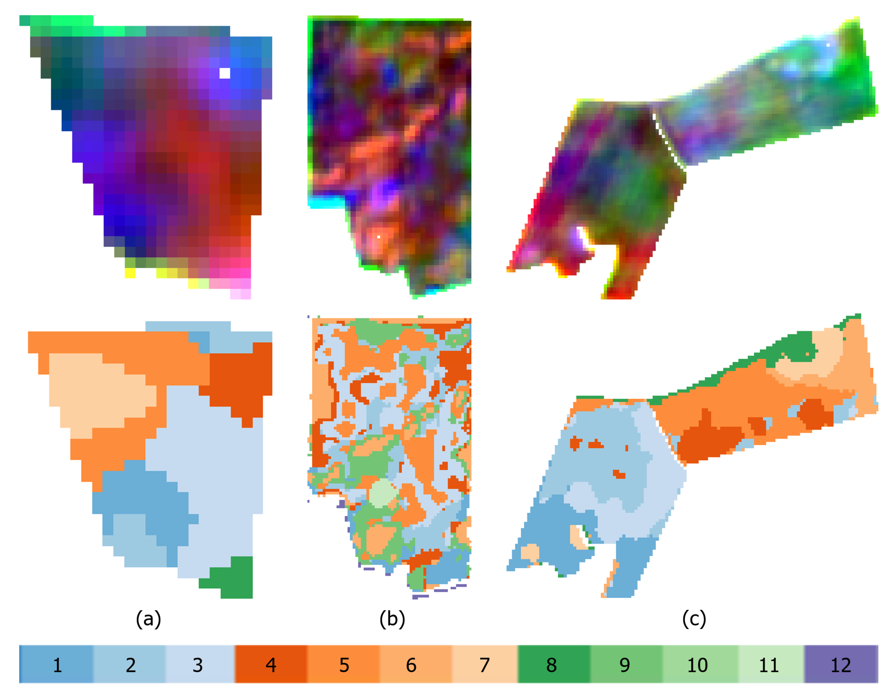
The index-RGB images show the heterogeneity within the fields (Figure 4). In these index-RGB images, every color (i.e., red, orange, pink, etc.) corresponds to a soil characteristic reflecting a similar temporal signature for the combined S1 and S2 input data.
Afterward, this information is used to break down the image into soil zones (second row of Figure 4). The color-coding in the figures is chosen based on the number of zones that are calculated for that field. According to the soil zoning analysis on the fields that belong to the first campaign, Hasler has six, Kreuzhuegel has twelve, and Quellenacker has eight zones. The varying number of zones shows that using the presented approach, the number of zones is related to the temporal-spectral heterogeneity of the field and soil, respectively, and not directly to its size.
Initial validation of the soil zoning approach was done by investigating soil profiles according to the German reference for soil mapping [47] and found distinctive differences supporting the zoning approach. Later on, a plausibility check of the zoning approach was done by presenting the derived zone maps to the owning farmers, during the SolumScire project meeting conducted on the 6 June 2019. The overall evaluation showed that more than 90% of the zones appear to reflect differences known or expected by the farmers reflecting natural background such as soil properties, hydrology parameters or other features like previous amelioration practices.
The incorrectly identified zones are likely related to changes in the soil profile not detectable by remote sensing, remaining plant residues, or the effect of infrastructures on the field border that affects the SAR scattering. Different crop performances reported by farmers might also be due to in-season varying nutrient availability, or to weather conditions affecting soil properties and plant growth at the respective location during the experiment.
4.2. Soil Property Prediction
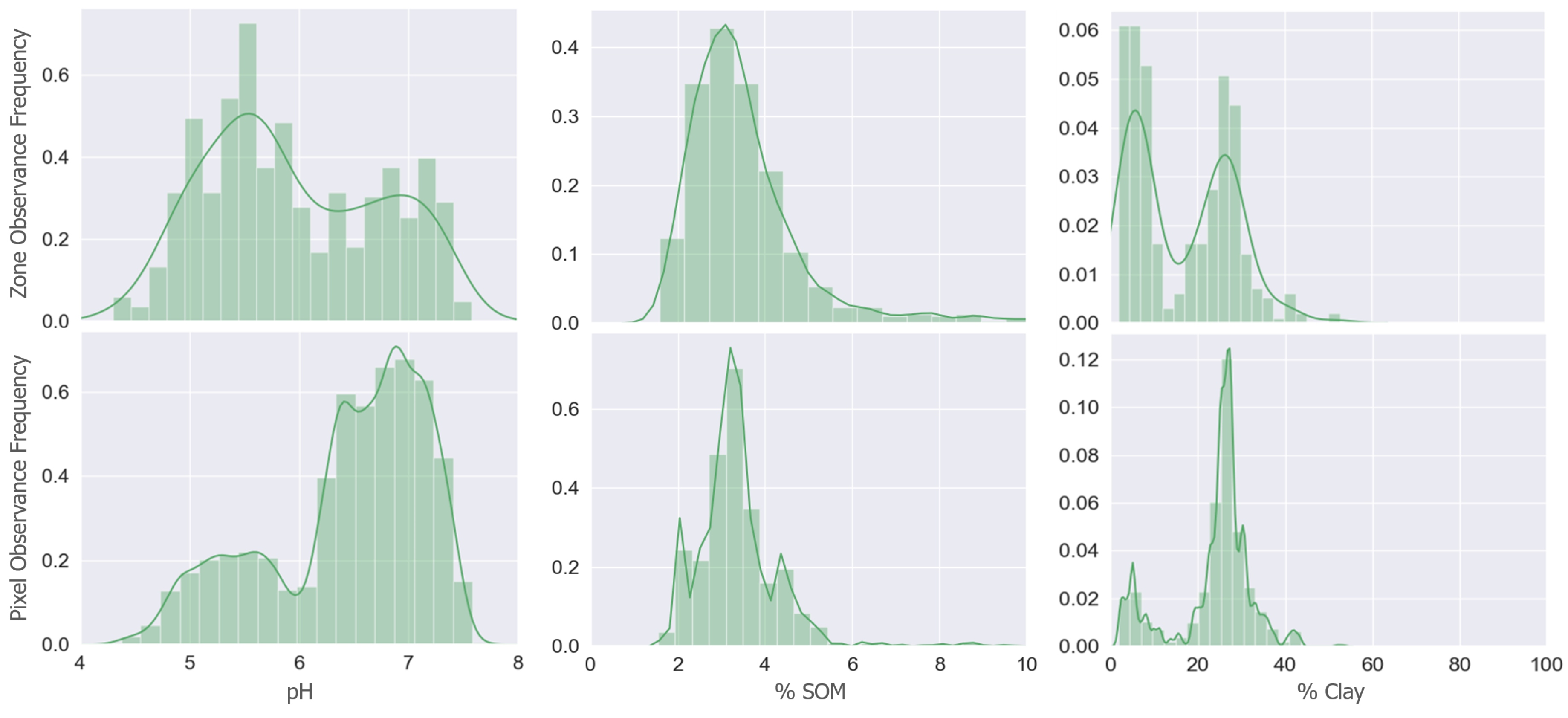
The soil property prediction algorithms were developed by training and optimizing a different model for each soil property and subsequent testing and validation. For the training and testing purposes, the data from the first sampling campaign was used. The first row of Figure 5 presents the probability distribution function for measurements taken per zone (pdf) for pH, SOM and clay content. In the histograms, pH and clay show a bi-modal distribution, while SOM shows a right-tailed uni-modal distribution. The pdf for pH, Figure 5, is calculated from 504 measurements and has peaks around 5.5 and 6.9. The pdf for SOM is calculated from 528 samples and has a peak of around 3.5. Lastly, the pdf for clay is calculated from 387 samples and has peaks around 5.6 and 25.8, corresponding to light sandy soils and heavier soils sampled in our study. Following the soil types, two peaks can also be found in the pdf for pH.
The augmentation of the RFR training and testing dataset requires the assumption of zones having similar soil properties. Hence, the zone level data is combined with the random variance of ±1.5% at each soil property value, resulting in a more realistic distribution and representation of the observed data at pixel level (Figure 5). Therefore the soil properties in the respective zone are weighted for their actual spatial distribution by remotely sensed information. This additional variance has led to a change in the pdf of the data presented to the RFR trainer.
For pH, pdf indicates most values to be between 6 and 7.5 and some less than 6. Optimal pH is dependent on SOM and clay content and is between 6 and 7 for most soils and can be lower for sandy soils. For the percentage of SOM, most samples are observed between 0, and 6 and only very few higher values are measured. Clay content observed in our study ranged from close to zero to shortly above 40%, reflecting a typical range found for arable soils in Europe.
The RFR models were trained using the satellite data as input and variance introduced ground measurement as output both at pixel-level. During the training procedure, leave-one-out cross-validation was applied for testing by selecting complete fields. In every iteration, the fields that correspond to at least 25% of the total sample size were randomly chosen for testing. Also, the fields that correspond to at least 20% of the total samples were left out for validation purposes.
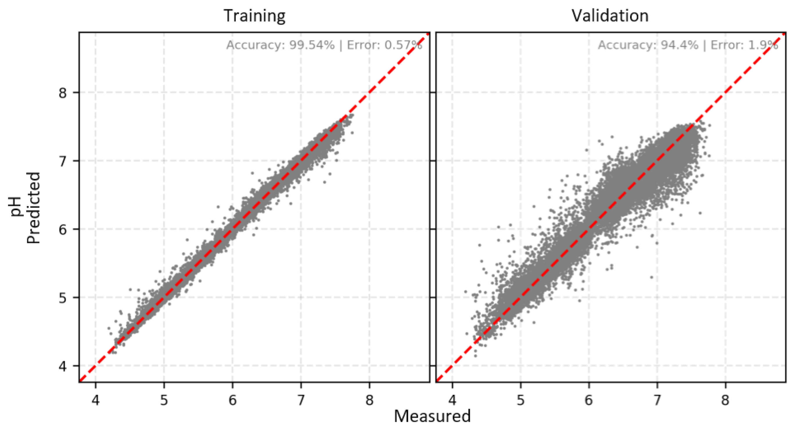
The accuracy of the pH model was observed to be very high (Figure 6). The training data has an R of 99.54% as accuracy and 0.57% mean absolute percentage error (mape) with its optimum parametrization. Validation analysis of the model resulted in an accuracy of 94.40% R and 1.9% mape. The difference between training and validation accuracy is small, indicating that over-fitting is not likely. The observed over or underestimation of pH values is relatively low compared to other soil pH mapping studies using satellite data [10]. The relative lower error may be a result of the higher spatial resolution of Sentinel input data compared to the Landsat information used in previous studies [10], but may also result from the focus on soils under intensive agricultural management in our dataset and the use of soil only information in the prediction algorithm.
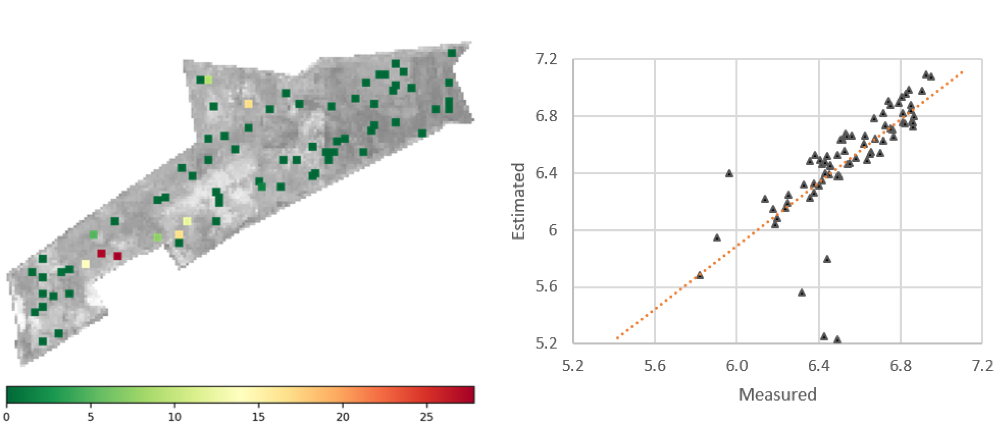
An independent validation analysis was conducted on the second sampling campaign for pH detection on the “Stadtfeld” field, including a total number of 76 samples. The point-wise pH values (Figure 7) of the topsoil shows a high prediction accuracy with less than 5% mape in more than 80% of the sampling points. The errors that are in the range of >5% might be observed due to missing data coverage in the training dataset. However, we cannot entirely exclude other factors such as soil amendments due to previous field management or edge effects in the remote sensing data such as wave shadow and reflection effects close to buildings affecting mostly SAR data [48].
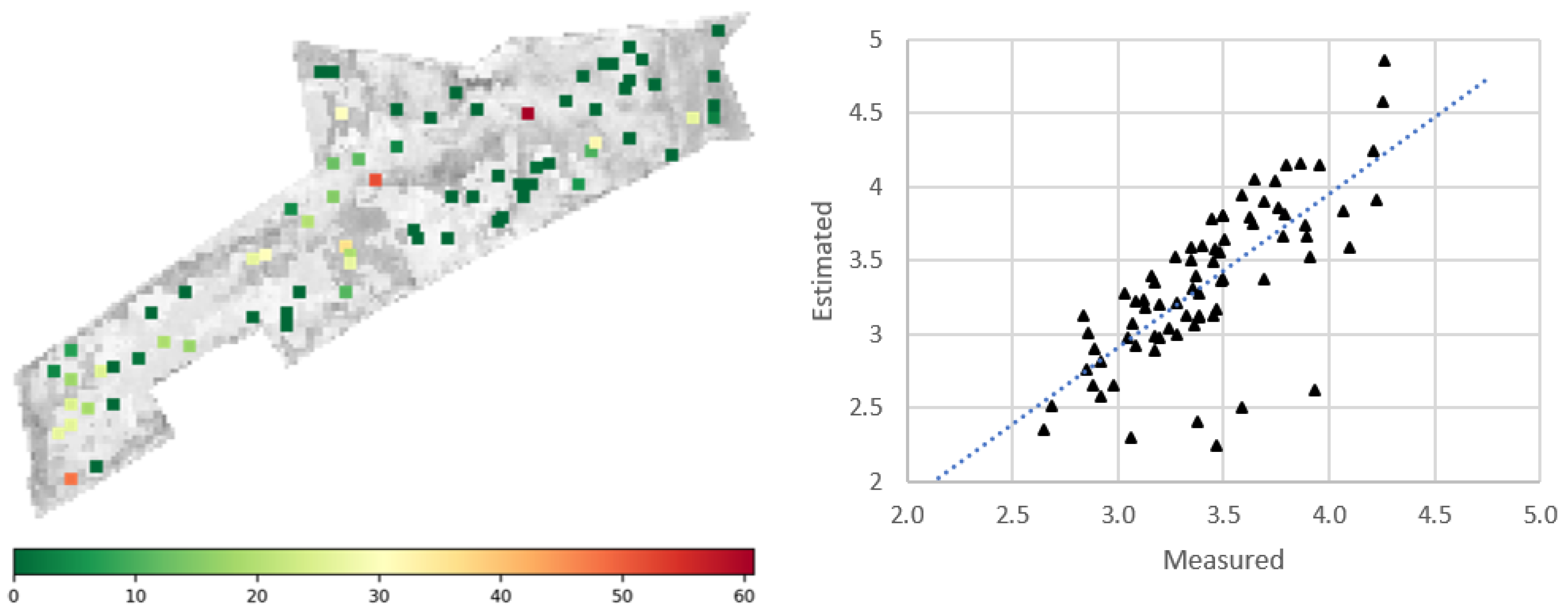
The prediction model for SOM content (in percentage) covers a range from about 1.5% to almost 10% (Figure 8). However, above 5.5 the data available for training, testing an validation is sparse. The training model has an R of 99.11% as accuracy and 1.33% mape with its optimum parametrization. Validation analysis of the model resulted in an accuracy of 89.0% R and 5.00% mape. The training and validation accuracy reflects the same pattern of having a lower dataset density in SOM above SOM of 5.5%. Some over and underestimation is found in the validation accuracy. However, the number of such observations is relatively low. Therefore, we consider the risk for over-fitting of the RFR model is relatively low. Nevertheless, the model can surely be improved by including more soil samples with SOM >5.5% in the future. Compared to previous studies predicting SOC facilitated by land use models and auxiliary data such as topography or climate data [11,49], the presented RFR model is capable of providing high accuracy prediction of SOM at pixel-level based on soil only remote sensing data.
The independent sampling campaign at the Stadtfeld field (Figure 9) reveals a good agreement for the majority of measured points. However, a larger error than observed for the pH mapping was found. Such a larger discrepancy of the predicted vs. measured SOM can be partly expected because SOM and its related remote sensed features are affected by more factors. These factors may cause (i) higher potential for variation and difference than for pH and clay content, (ii) show effect of crop residues on the field surface or (iii) contribution of less spectral features to the parameter prediction. Additionally, variable gradients of SOM in different soils might add a variation in the prediction. Consequently, a larger database would be needed to obtain a higher prediction quality.
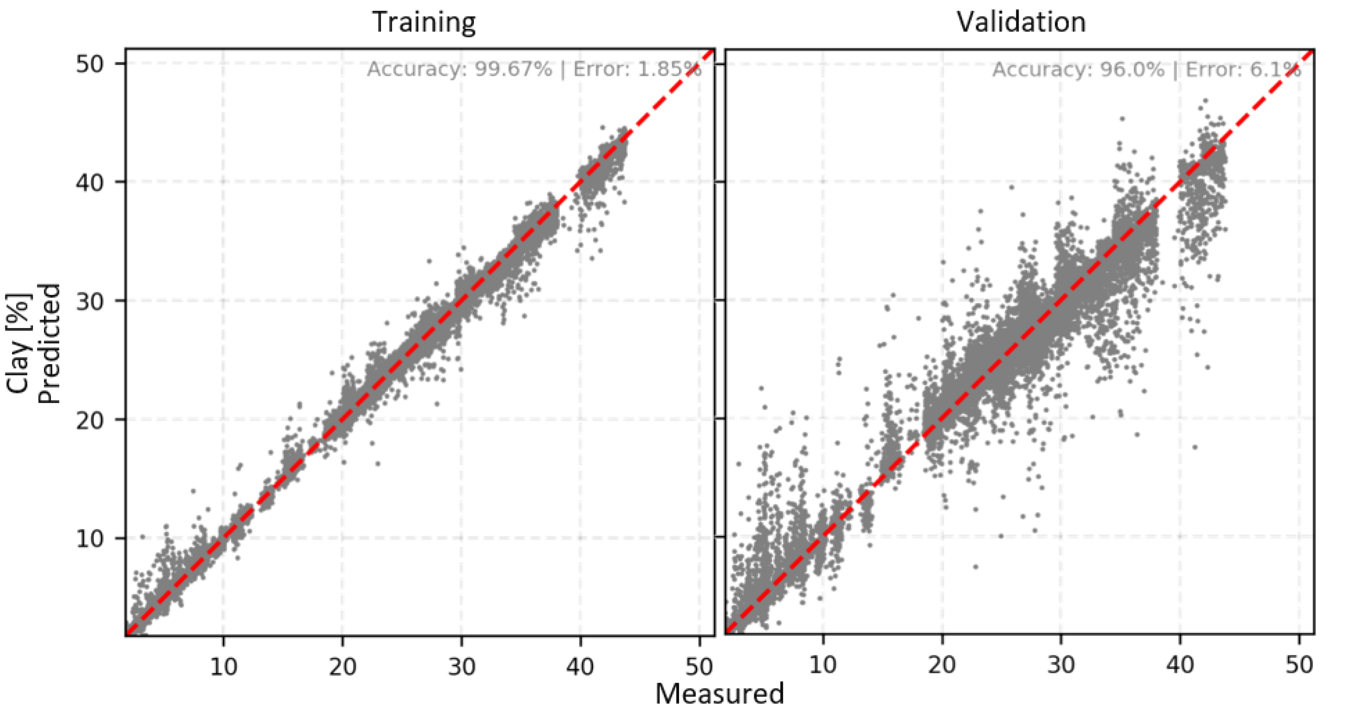
The prediction of clay content (Figure 10) also shows high accuracy in the training and validation set, having an R of 99.67% and mape of 1.85% with its optimum parametrization. Validation analysis of the model resulted in an accuracy of 96.00% R and a 6.1% mape being, which in the prediction than that obtained for SOM, but not as good as for pH. The observed over, or underestimation in the validation set can be considered as small, making it plausible to assume that no significant over-fitting of the RFR model is present. Compared to other satellite remote sensing approaches for clay content prediction [9], the presented model has excellent performance allowing for practical uses. The reasons for the better performance is likely found in the soil only remote sensing input data for model development. Prediction accuracy of laboratory spectroscopy for clay content is usually very high [50,51] being based on homogenized soil samples independent of soil management and use as satellite data. Further, the restriction of the dataset to arable field soils can be another reason for the higher predication power observed in our study compared to large scale mapping approaches of soil properties based on a broad range of land use and land cover data [9].
4.3. In Field Soil Property Distribution
Three fields that are sampled during the first field campaign were selected to show potential output and plausibility of the presented methodology. The results are presented using maps that are generated for measured and predicted soil property, predicted percentage error, and indices that reflect the vegetation performance, NDVI and SVI. Table 1, shows the summary of the soil and vegetation characteristics for the fields that are sampled during the first field campaign.
4.3.1. Hasler, Switzerland
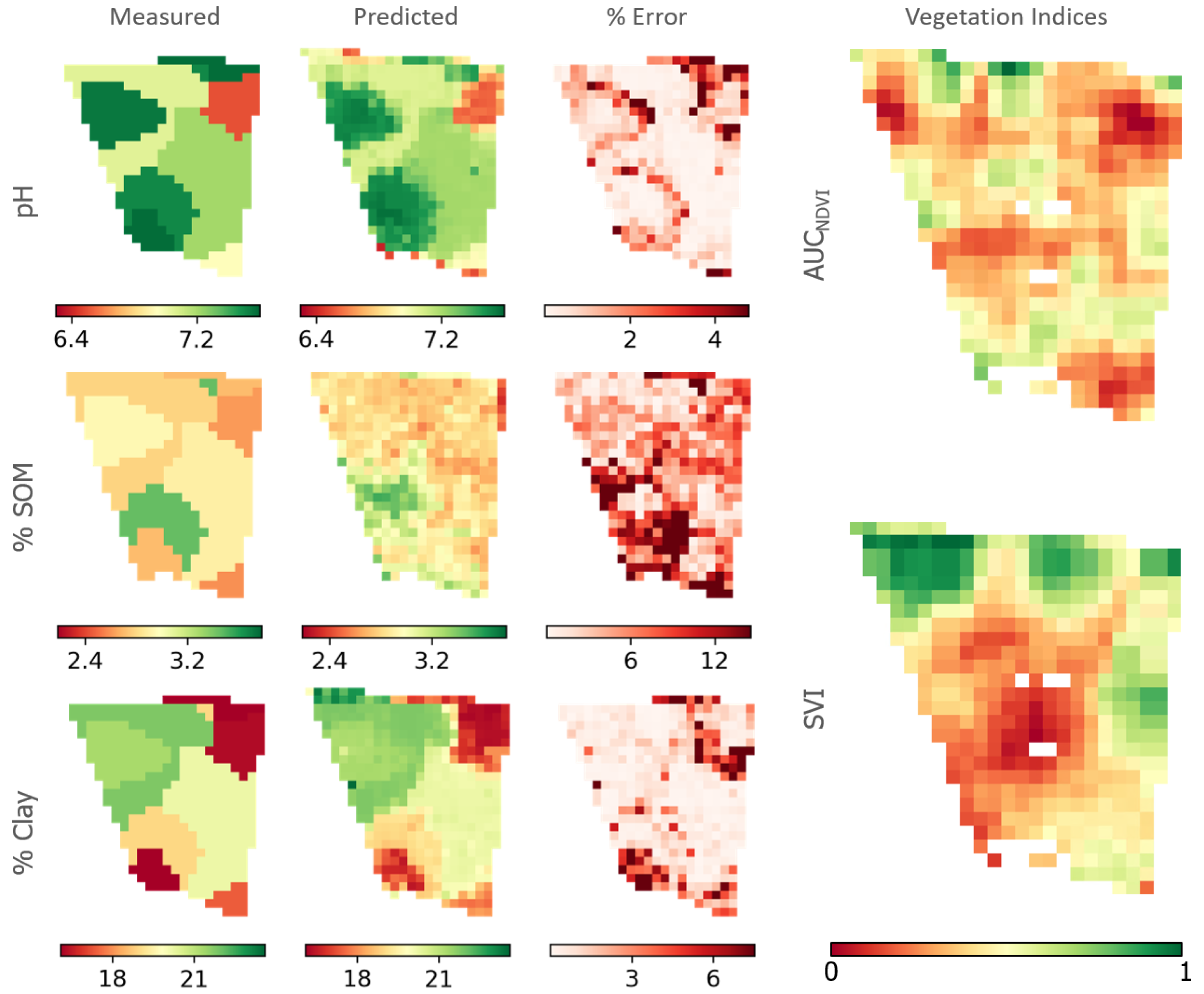
In the Hasler field, predicted pH and clay content mainly follow the soil zones initially identified by the unsupervised methodology (Figure 11). The distribution of SOM is less clearly bound to those zones. The observed error patterns also reflect this condition. For pH and clay, the more significant errors can be found at the zone borders. In contrast, for SOM, errors are more distributed in the field, indicating a considerable small scale variability. The higher variability can be related to many factors, including soil-structure [52] but also field management and climate variables [53,54]. If field management and climate data is available for analysis, it can be used in an updated model and potentially increase prediction accuracy. However, the potential improvement and best methodology remains to be investigated.
The crop properties seem less clearly bound to the observed soil zones. A low pH and clay content seem to be linked to lower biomass productivity indicated by the NDVI, but not necessarily linked to the lower crop density in the winter wheat field. The SVI indicates the morphology and canopy density differences around the region with the highest SOM. Besides, it shows lower values in the lowest region of the field being an effect of topography. Particularly in sandy soils, as found in the Hasler field, higher SOM can buffer the low storage capacity for water and nutrients, which may lead to the higher canopy and morphology changes observed in the other parts of the field.
4.3.2. Kreuzhuegel, Germany
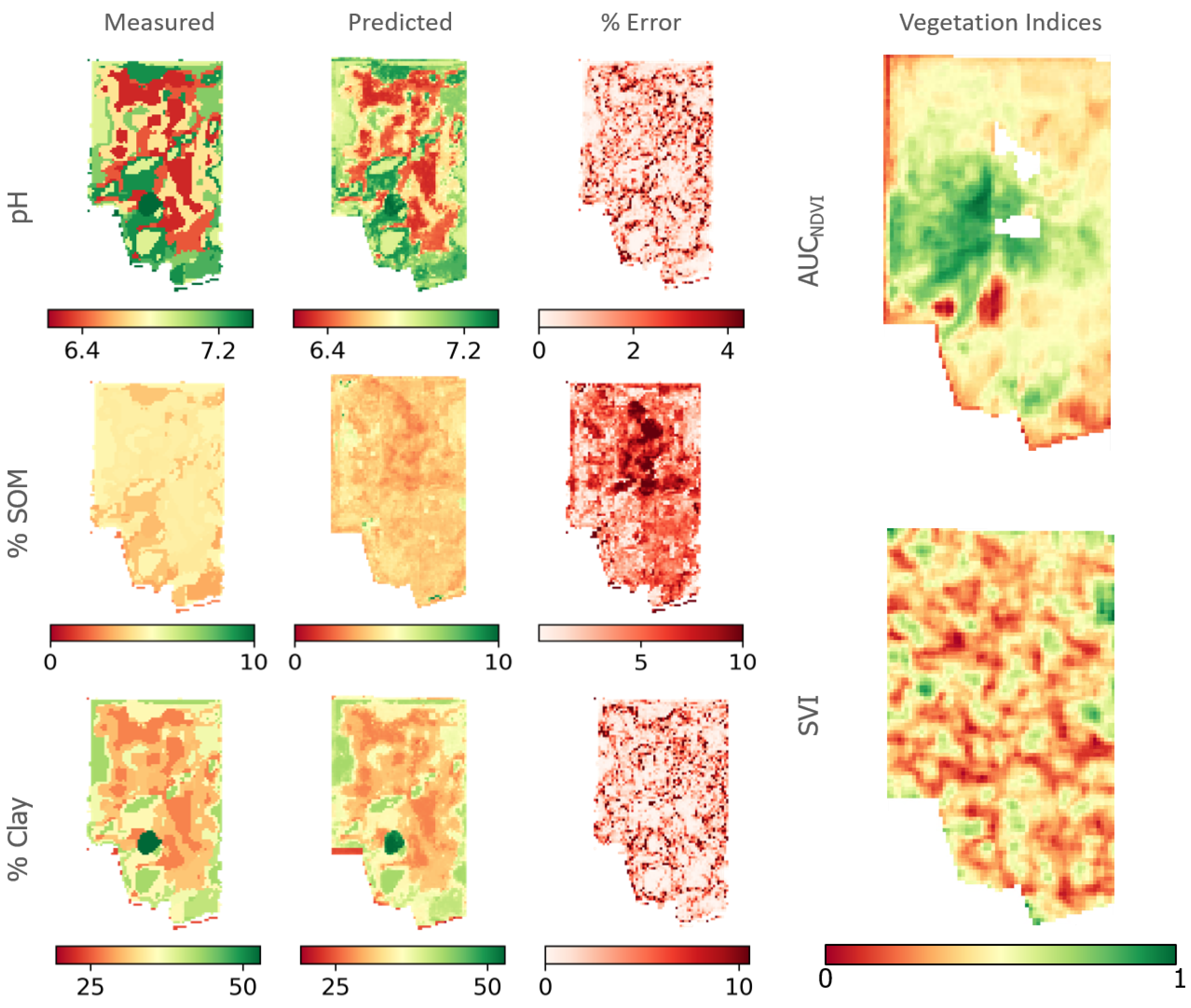
The field Kreuzhuegel shows a very high number of distinct zones, mainly affected by pH and clay content having a positive correlation (Figure 12). The homogeneously distributed SOM shows relatively high values in the field. The large variation is originating from the strong heterogeneity of the sub-soil silt and clay content.
The plant indicators partly reflect those zones, particularly SVI, but also show different patterns potentially indicating differences in the soil profile and the root-able soil depth. The biomass productivity indicated by NDVI reflects a low growth in the clay lens zone but also the highest growth in the green area not fully delineated by the pH or clay content.
4.3.3. Quellenacker, Germany
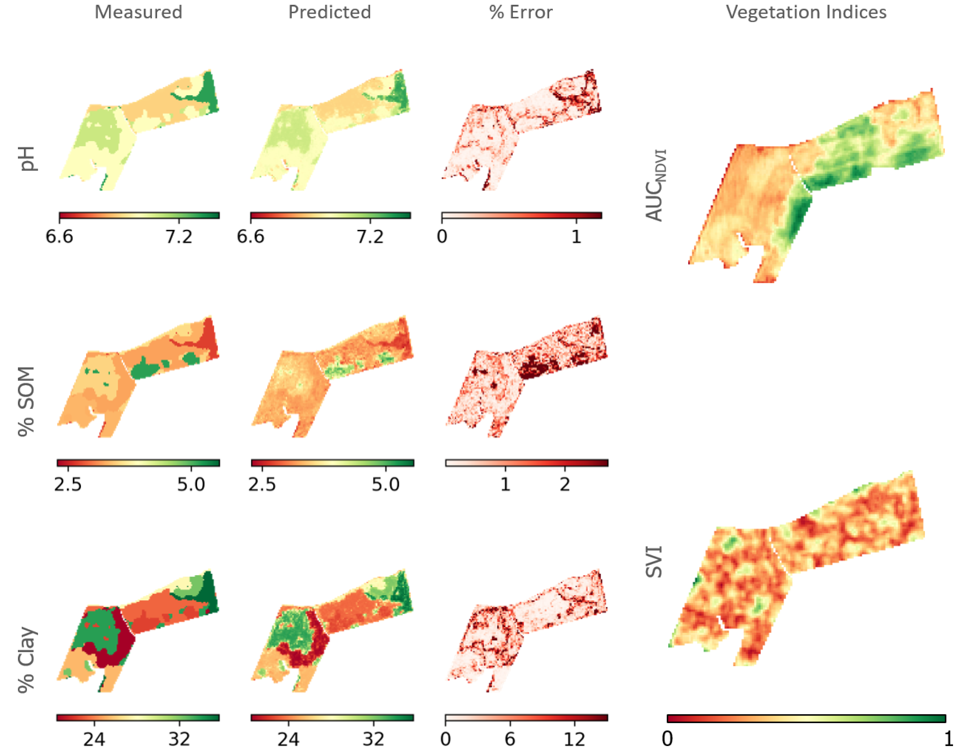
In the Quellenacker, distinct soil zones are observed that are related to the evaluated soil properties. However, here the three soil properties pH, SOM and clay reflect the zone patterns indicating more pronounced differences between soils (Figure 13). As expected, the high pH values are linked to higher clay and, additionally, to lower SOM.
Similar to the previously discussed fields, the canopy density indicator SVI shows no distinct relation to the zones, likely indicating that crop growth was mostly homogeneous. In contrast, the biomass productivity indication (NDVI) reflects apparent differences in the field. The higher biomass productivity was in the regions indicating higher SOM, clay content below 25, and pH below 7. As discussed above, the partial mismatch of soil and plant property zones may reflect differences caused by differences in the subsoil and topographic differences in the field not reflected by the presented algorithm.
4.4. Future Work and Potential Applications
The presented study shows the high potential of satellite-based prediction of soil properties for precision agriculture. In contrast to previous soil mapping studies [9,11] actual satellite missions such as the Copernicus have higher spatial and temporal resolution applicable for time-dependent spatial applications such as precision crop management. Examples for such uses are the application of lime to adjust pH and the buffer capacity of the soils and fertilizer application. The prediction of lime or fertilizer demand usually makes use of soil pH, SOM, and clay contents in most countries. Thus, the methodology described here to predict the three parameters should be applied using existing methodology supported by satellite input data to inform variable rate application of lime and fertilizer.
Soil pH and buffer capacity, for instance, can be modeled as a function of SOM and clay content [55]. Such a model is applied for a comprehensive set of soils and soil sample information combined in a geographic information system (GIS) to map the spatial variability of soil pH and predict lime application demand in a large agricultural field. The presented soil property mapping allows for much greater detail and even seasonal mapping depending on the crop and availability of satellite data.
Similarly, the classification of the phosphorus fertility of soils is often based on clay and pH, affecting plant availability of phosphorus [56]. Knowing the spatial extent of these properties would not only allow adjustment of phosphorus fertilization based on these parameters without additional information but also based on soil sampling followed by phosphorus extraction and interpretation using the respective national interpretation schemes.
A third example is the prediction of the initial nitrogen fertilizer application as practiced for many crops. The required amount of nitrogen cannot be based on vegetation status as it is used for in-season fertilization. However, it can be based on known average crop nitrogen uptake and soil mineral nitrogen available to the plant determined by soil sampling [57]. Sometimes the prediction of nitrogen available to the plant is done with basic models informed by pH, SOM, and clay content [58]. Mineralization models often combine these soil properties with climate and cropping information to predict potential nitrogen mineralization to reduce the amount of N to be applied [59].
The presented study also shows that the sole basis of field management zones on either soil or vegetation information should be challenged. While soil zones often refer to regions in a field that need different agricultural management, they usually do not respect actual or later crop development or release of nutrients. In contrast, management zones based on seasonal biomass maps or vegetation indices reflect the actual situation but might under-represent plant-soil interactions, particularly during seasons with different crops and weather conditions.
Future studies should focus on optimizing informed prediction of crop fertilizer demand based on soil and vegetation information and evaluate the potential of financial gains and reduction of climate and environmental risks posed by nutrient losses. Another field of interest is the improvement of SOM prediction accuracy to allow monitoring of SOM changes even in relatively short term and eventually soil carbon sequestration.
4.5. Limits of the Method and Potential Adaptation
The presented methodology is partially limited by the use of MS information, which restricts the method to periods without cloud cover. Cloud cover can be substantial between autumn and spring in Switzerland [60] and Germany. Although, SAR data may partly balance this, it can be assumed that the MS spectrum plays still a pivotal role in soil property prediction. Including auxiliary data, such as topographic information like slope altitude and topographic wetness index, might further improve prediction of soil properties and delineation of management zones likewise under clouded and non-clouded situations.
The soil zoning and property prediction can also be improved by identifying and stratifying the input variables such as the satellite-derived input channels or auxiliary information for specific soil properties. However, this can improve performance but also limit sensitivity to selected properties. Another approach could be the use of a floating input according to the highest variability of observed properties.
However, reliability for the prediction of some soil properties can be low as a result of the significant variance of parameters influencing the target soil property to be predicted. Such variance is often indirectly reflected by the number of spectral input features usable for the parameter prediction. This condition seems more pronounced for dynamic soil properties, such as SOM, which can change fast.
Such difficulties can potentially be overcome by the use of much larger data sets covering more seasons, and field situations or by local adjustment of the model by support samples. The concept of taking a limited set of soil samples to improve the model and thus improve pixel-wise predictions for specific fields is particularly interesting. Such a method limits the number of samples needed to be taken per field compared to historical sampling plans and delivers additional data to improve the model in the long term. Additionally, an informed sampling procedure facilitates optimal placements of sampling points according to the distribution and spread of the initially predicted variables.
4.6. Soil and Management Zoning in Agriculture
Existing soil maps—if digitized at all—are sometimes lacking scalability and are not always up-to-date [46] or available. Additionally, soil maps are often not optimized for agricultural use needing data processing or transformation by experts to allow intuitive interpretation by the farmer.
Many satellite-based field zoning approaches use biomass as the primary decision parameter. However, biomass is dependent on crop properties and growth conditions, comprising variety-specific crop traits, soil properties, and seasonal weather differences, which strongly interact as discussed above [28]. The same is true for other sources of information used for soil and management zoning in the last two decades, such as apparent electrical conductivity and yield maps. Often these methods reflect differences in soil characteristics or crop growth, but not the underlying reasons. However, these have to be known in order to make appropriate agronomic decisions. Nevertheless, many indicators for field heterogeneity are used successfully for precision agriculture and variable rate application methodology in particular.
Expert derived zoning, on the other hand, has proven to be a valuable tool for precision farming. The expert can use a selection of tools for mapping [61], including the mentioned above, and select and eventually combine the most appropriate sources of information [46,55]. However, expert-based zoning is time-consuming and expensive, and it often requires laborious work in the field and data analysis. Additionally, the degree of detail is often not as high as many imaging or remote sensing approaches, as presented in Figure 3. This situation is likely to change with tools like the presented soil zoning becoming available user friendly and widely compatible.
The focus of the presented soil zoning approach lies in the unsupervised use of spectral data from bare or nearly bare soils. For many agricultural applications, knowledge of soil properties is essential. The availability of such information is particularly interesting for the three investigated parameters pH, SOM, and clay content. Their spatial distribution can be used for variable rate fertilization of lime, phosphorus, and nitrogen, as described above.
The approach shown here is finally combining spectral data and laboratory analysis to explain soil heterogeneity. It is somewhat more time consuming than methods only indicating heterogeneity because of the laborious and costly soil sampling and analysis. These points make it more expensive than other maps taken on-the-go but also more reliable for agronomic decisions. However, the costs are not higher as with traditional soil sampling and analysis performed on the farm. A decline of the costs can be expected with increasing numbers of soil analyses and due to use of new lab techniques such as spectroscopy, which will help to improve the large scale prediction of soil properties and its application for agronomic uses.
5. Conclusions
This research presents a new remote sensing-based soil zoning and property prediction algorithm. For this purpose, MS and SAR images were used from the Copernicus mission making use of high-resolution satellite agricultural field imagery obtained during the plant free periods, consisting of mostly soil input data. The retrieved products of the presented algorithms include predicted pH, SOM, and clay content of each pixel in a field. Such products allow informed soil sampling and precision agriculture applications such as variable-rate lime, phosphorus, and nitrogen fertilization. Additionally, by considering the likelihood of seasonal changes in the soil and vegetation properties, the algorithm can be adapted to detect dynamic changes in the soil properties that might support the monitoring of SOM and soil acidity.
Author Contributions
Conceptualization and methodology, O.Y., F.L. (Frank Lorenz), P.F., F.L. (Frank Liebisch); organizing ground campaigns and lab analysis, F.L. (Frank Lorenz), P.F., F.L. (Frank Liebisch); code development and analysis, O.Y.; writing—original draft preparation, O.Y. and F.L. (Frank Liebisch); writing—review and editing, O.Y., F.L. (Frank Lorenz), F.L. (Frank Liebisch); visualization, O.Y.; supervision, F.L. (Frank Liebisch); project administration, P.F.; funding acquisition, P.F. All authors have read and agreed to the published version of the manuscript.
Funding
This research was funded under the name SolumScire 50% by ESA and 50% by the SolumScire consortium being AgriCircle, LUFA Nordwest, ETH Zürich Group of CropScience. AgriCircle received additional funding by Climate-KIC.
Acknowledgments
The authors would like to thank the members of the Google Earth Engine team for providing the Sentinel data, the supportive farmers of the SolumScire project: Christian Münchhoff, Falk Lieder and Jens Hartig for their field expertise and soil analysis teams located in ETH Zurich and LUFA and Agroscope for conducting the soil characterization and Achim Walter, Christ Johannes Gilli, Brigitta Herzog (ETH Zürich), Noura Fajraoui, Rodrigo Principe, Tomasz Szymczyszyn (AgriCircle) and Marlies Sommer (Agroscope Soil Protection Group) for their support.
Conflicts of Interest
The authors declare no conflict of interest.
Abbreviations
The following abbreviations are used in this manuscript:
| ESA | European Space Agency | GEE | Google Earth Engine |
| GIS | Geographic Information System | GRD | Ground Range Detected |
| MS | Multi-Spectral | NDVI | Normalized Difference Vegetation Index |
| NIR | Near-Infrared | PCA | Principle Component Analysis |
| Probability Distribution Function | PolSAR | Polarimetric Synthetic Aperture Radar | |
| ROI | Region of Interest | SOM | Soil Organic Matter |
| S1 | Sentinel-1 satellite data | S2 | Sentinel-2 satellite data |
| SVI | SAR Vegetation Index | AUC | Area Under the Curve |
References
- Mulla, D.J. Twenty five years of remote sensing in precision agriculture: Key advances and remaining knowledge gaps. Biosyst. Eng. 2013, 114, 358–371. [Google Scholar] [CrossRef]
- Ge, Y.; Thomasson, J.A.; Sui, R. Remote sensing of soil properties in precision agriculture: A review. Front. Earth Sci. 2011, 5, 229–238. [Google Scholar] [CrossRef]
- Pierce, F.J.; Nowak, P. Aspects of Precision Agriculture. In Advances in Agronomy; Elsevier: Amsterdam, The Netherlands, 1999; Volume 67, pp. 1–85. [Google Scholar]
- Zhang, N.; Wang, M.; Wang, N. Precision agriculture—A worldwide overview. Comput. Electron. Agric. 2002, 36, 113–132. [Google Scholar] [CrossRef]
- Gebbers, R.; Adamchuk, V.I. Precision agriculture and food security. Science 2010, 327, 828–831. [Google Scholar] [CrossRef]
- Delegido, J.; Verrelst, J.; Alonso, L.; Moreno, J. Evaluation of sentinel-2 red-edge bands for empirical estimation of green LAI and chlorophyll content. Sensors 2011, 11, 7063–7081. [Google Scholar] [CrossRef] [Green Version]
- Clevers, J.G.; Gitelson, A.A. Remote estimation of crop and grass chlorophyll and nitrogen content using red-edge bands on Sentinel-2 and-3. Int. J. Appl. Earth Obs. Geoinf. 2013, 23, 344–351. [Google Scholar] [CrossRef]
- Verrelst, J.; Muñoz, J.; Alonso, L.; Delegido, J.; Rivera, J.P.; Camps-Valls, G.; Moreno, J. Machine learning regression algorithms for biophysical parameter retrieval: Opportunities for Sentinel-2 and-3. Remote Sens. Environ. 2012, 118, 127–139. [Google Scholar] [CrossRef]
- Ballabio, C.; Panagos, P.; Monatanarella, L. Mapping topsoil physical properties at European scale using the LUCAS database. Geoderma 2016, 261, 110–123. [Google Scholar] [CrossRef]
- Ballabio, C.; Lugato, E.; Fernández-Ugalde, O.; Orgiazzi, A.; Jones, A.; Borrelli, P.; Montanarella, L.; Panagos, P. Mapping LUCAS topsoil chemical properties at European scale using Gaussian process regression. Geoderma 2019, 355, 113912. [Google Scholar] [CrossRef]
- Yigini, Y.; Panagos, P. Assessment of soil organic carbon stocks under future climate and land cover changes in Europe. Sci. Total Environ. 2016, 557, 838–850. [Google Scholar] [CrossRef]
- Yuzugullu, O.; Erten, E.; Hajnsek, I. Estimation of rice crop height from X-and C-band PolSAR by metamodel-based optimization. IEEE J. Sel. Top. Appl. Earth Obs. Remote Sens. 2017, 10, 194–204. [Google Scholar] [CrossRef] [Green Version]
- McNairn, H.; Brisco, B. The application of C-band polarimetric SAR for agriculture: A review. Can. J. Remote Sens. 2004, 30, 525–542. [Google Scholar] [CrossRef]
- Lopez-Sanchez, J.M.; Ballester-Berman, J.D. Potentials of polarimetric SAR interferometry for agriculture monitoring. Radio Sci. 2009, 44, 1–20. [Google Scholar] [CrossRef] [Green Version]
- Franceschetti, G.; Lanari, R. Synthetic Aperture Radar Processing; CRC Press: Boca Raton, FL, USA, 2018. [Google Scholar]
- Baghdadi, N.; Gaultier, S.; King, C. Retrieving surface roughness and soil moisture from synthetic aperture radar (SAR) data using neural networks. Can. J. Remote Sens. 2002, 28, 701–711. [Google Scholar] [CrossRef]
- Srivastava, H.S.; Patel, P.; Manchanda, M.; Adiga, S. Use of multiincidence angle RADARSAT-1 SAR data to incorporate the effect of surface roughness in soil moisture estimation. IEEE Trans. Geosci. Remote Sens. 2003, 41, 1638–1640. [Google Scholar] [CrossRef]
- Baghdadi, N.; Cresson, R.; El Hajj, M.; Ludwig, R.; La Jeunesse, I. Estimation of soil parameters over bare agriculture areas from C-band polarimetric SAR data using neural networks. Hydrol. Earth Syst. Sci. 2012, 16, 1607–1621. [Google Scholar] [CrossRef] [Green Version]
- Erten, E.; Lopez-Sanchez, J.M.; Yuzugullu, O.; Hajnsek, I. Retrieval of agricultural crop height from space: A comparison of SAR techniques. Remote Sens. Environ. 2016, 187, 130–144. [Google Scholar] [CrossRef] [Green Version]
- Malhi, S.; Grant, C.; Johnston, A.; Gill, K. Nitrogen fertilization management for no-till cereal production in the Canadian Great Plains: A review. Soil Tillage Res. 2001, 60, 101–122. [Google Scholar] [CrossRef]
- McCauley, A.; Jones, C.; Jacobsen, J. Soil pH and organic matter. Nutr. Manag. Modul. 2009, 8, 1–12. [Google Scholar]
- Carlen, C.; Flisch, R.; Gilli, C.; Huguenin-Elie, O.; Kuster, T.; Latsch, A.; Mayer, J.; Neuweiler, R.; Richner, W.; Sokrat, S.; et al. Principles of Fertilization of Agricultural Crops in Switzerland; Agroscope: Berne, Switzerland, 2017. [Google Scholar]
- Reimann, C.; Siewers, U.; Tarvainen, T.; Bityukova, L.; Eriksson, J.; Giucis, A.; Gregorauskiene, V.; Lukashev, V.K.; Matinian, N.N.; Pasieczna, A. Agricultural Soils in Northern Europe; Schweizerbartsche Verlagsbuchhandlung: Stuttgart, Germany, 2003. [Google Scholar]
- Takeda, A.; Kimura, K.; Yamasaki, S.i. Analysis of 57 elements in Japanese soils, with special reference to soil group and agricultural use. Geoderma 2004, 119, 291–307. [Google Scholar] [CrossRef]
- Chesworth, W. Encyclopedia of Soil Science; Springer Science & Business Media: Berlin/Heidelberg, Germany, 2007. [Google Scholar]
- Ortega, R.A.; Santibáñez, O.A. Determination of management zones in corn (Zea mays L.) based on soil fertility. Comput. Electron. Agric. 2007, 58, 49–59. [Google Scholar] [CrossRef]
- Kurtener, D.; Yakushev, V.; Torbert, H.; Kruger, E. Zoning of an Agricultural Field using a Fuzzy Indicator Model. In Proceedings of the European Conference on Precision Agriculture, Prague, Czech Republic, 11–14 July 2011. [Google Scholar]
- Mzuku, M.R.K.; Reich, R.; Inman, D.; Smith, F.; MacDonald, L. Spatial Variability of Measured Soil Properties across Site-Specific Management Zones. Soil Sci. Soc. Am. J. 2005, 69, 1572–1579. [Google Scholar] [CrossRef] [Green Version]
- Fortes, R.; Millán, S.; Prieto, M.; Campillo, C. A methodology based on apparent electrical conductivity and guided soil samples to improve irrigation zoning. Precis. Agric. 2015, 16, 441–454. [Google Scholar] [CrossRef]
- Schepers, A.R.; Shanahan, J.F.; Liebig, M.A.; Schepers, J.S.; Johnson, S.H.; Luchiari, A. Appropriateness of Management Zones for Characterizing Spatial Variability of Soil Properties and Irrigated Corn Yields across Years. Agron. J. 2004, 96, 195–203. [Google Scholar] [CrossRef] [Green Version]
- Gorelick, N.; Hancher, M.; Dixon, M.; Ilyushchenko, S.; Thau, D.; Moore, R. Google Earth Engine: Planetary-scale geospatial analysis for everyone. Remote Sens. Environ. 2017, 202, 18–27. [Google Scholar] [CrossRef]
- El Hajj, M.; Baghdadi, N.; Zribi, M.; Bazzi, H. Synergic use of Sentinel-1 and Sentinel-2 images for operational soil moisture mapping at high spatial resolution over agricultural areas. Remote Sens. 2017, 9, 1292. [Google Scholar] [CrossRef] [Green Version]
- Carlotto, M.J.; Lazaroff, M.B.; Brennan, M.W. Multispectral image processing for environmental monitoring. Proc. SPIE 1993, 1819, 113–124. [Google Scholar]
- Forschungsanstalten, V. Methodenbuch Band 1: Die Untersuchung von Böden; VDLUFA: Darmstadt, Germany, 1991. [Google Scholar]
- Yang, R.M.; Guo, W.W. Using time-series Sentinel-1 data for soil prediction on invaded coastal wetlands. Environ. Monit. Assess. 2019, 191, 462. [Google Scholar] [CrossRef]
- Blasch, G.; Spengler, D.; Hohmann, C.; Neumann, C.; Itzerott, S.; Kaufmann, H. Multitemporal soil pattern analysis with multispectral remote sensing data at the field-scale. Comput. Electron. Agric. 2015, 113, 1–13. [Google Scholar] [CrossRef] [Green Version]
- Jolliffe, I. Principal Component Analysis; Springer: Berlin/Heidelberg, Germany, 2011. [Google Scholar]
- MacQueen, J. Some Methods for Classification and Analysis of Multivariate Observations. In Proceedings of the Fifth Berkeley Symposium on Mathematical Statistics and Probability, Berkeley, CA, USA, 21 June–18 July 1965 and 27 December 1965–7 January 1966; UCP: Berkeley, CA, USA, 1967; pp. 281–297. [Google Scholar]
- Kodinariya, T.M.; Makwana, P.R. Review on determining number of Cluster in K-Means Clustering. Int. J. 2013, 1, 90–95. [Google Scholar]
- Svetnik, V.; Liaw, A.; Tong, C.; Culberson, J.C.; Sheridan, R.P.; Feuston, B.P. Random forest: A classification and regression tool for compound classification and QSAR modeling. J. Chem. Inf. Comput. Sci. 2003, 43, 1947–1958. [Google Scholar] [CrossRef] [PubMed]
- Pedregosa, F.; Varoquaux, G.; Gramfort, A.; Michel, V.; Thirion, B.; Grisel, O.; Blondel, M.; Prettenhofer, P.; Weiss, R.; Dubourg, V.; et al. Scikit-learn: Machine Learning in Python. J. Mach. Learn. Res. 2011, 12, 2825–2830. [Google Scholar]
- Rouse, J., Jr. Monitoring the Vernal Advancement and Retrogradation (Green Wave Effect) of Natural Vegetation. In Technical Report; NASA: Washington, DC, USA, 1972. [Google Scholar]
- Gao, Q.; Zribi, M.; Escorihuela, M.J.; Baghdadi, N.; Segui, P.Q. Irrigation mapping using Sentinel-1 time series at field scale. Remote Sens. 2018, 10, 1495. [Google Scholar] [CrossRef] [Green Version]
- Zhang, Y.; Gong, J.; Sun, K.; Yin, J.; Chen, X. Estimation of soil moisture index using multi-temporal Sentinel-1 images over Poyang Lake ungauged zone. Remote Sens. 2018, 10, 12. [Google Scholar] [CrossRef] [Green Version]
- Weather API Meteomatics. Available online: https://www.meteomatics.com/weather-api/ (accessed on 11 December 2019).
- Lorenz, F.; Münchhoff, K. Teilflaechen Bewirtschaften Schritt für Schrit; DLG-Verlag: Frankfurt am Main, Germany, 2015. [Google Scholar]
- Sponagel, H. Bodenkundliche Kartieranleitung: Mit 103 Tabellen; Schweizerbart: Stuttgart, Germany, 2005. [Google Scholar]
- Moreira, A.; Prats-Iraola, P.; Younis, M.; Krieger, G.; Hajnsek, I.; Papathanassiou, K.P. A tutorial on synthetic aperture radar. IEEE Geosci. Remote Sens. Mag. 2013, 1, 6–43. [Google Scholar] [CrossRef] [Green Version]
- Stumpf, F.; Keller, A.; Schmidt, K.; Mayr, A.; Gubler, A.; Schaepman, M. Spatio-temporal land use dynamics and soil organic carbon in Swiss agroecosystems. Agric. Ecosyst. Environ. 2018, 258, 129–142. [Google Scholar] [CrossRef]
- Sørensen, L.; Dalsgaard, S. Determination of clay and other soil properties by near infrared spectroscopy. Soil Sci. Soc. Am. J. 2005, 69, 159–167. [Google Scholar] [CrossRef]
- Rossel, R.V.; Cattle, S.R.; Ortega, A.; Fouad, Y. In situ measurements of soil colour, mineral composition and clay content by vis–NIR spectroscopy. Geoderma 2009, 150, 253–266. [Google Scholar] [CrossRef]
- Six, J.; Paustian, K. Aggregate-associated soil organic matter as an ecosystem property and a measurement tool. Soil Biol. Biochem. 2014, 68, A4–A9. [Google Scholar] [CrossRef]
- Alexandrov, V.; Hoogenboom, G. The impact of climate variability and change on crop yield in Bulgaria. Agric. For. Meteorol. 2000, 104, 315–327. [Google Scholar] [CrossRef]
- Maracchi, G.; Sirotenko, O.; Bindi, M. Impacts of present and future climate variability on agriculture and forestry in the temperate regions: Europe. Clim. Chang. 2005, 70, 117–135. [Google Scholar] [CrossRef]
- Weaver, A.; Kissel, D.; Chen, F.; West, L.; Adkins, W.; Rickman, D.; Luvall, J. Mapping soil pH buffering capacity of selected fields in the coastal plain. Soil Sci. Soc. Am. J. 2004, 68, 662–668. [Google Scholar] [CrossRef]
- Jordan-Meille, L.; Rubæk, G.H.; Ehlert, P.; Genot, V.; Hofman, G.; Goulding, K.; Recknagel, J.; Provolo, G.; Barraclough, P. An overview of fertilizer-P recommendations in Europe: Soil testing, calibration and fertilizer recommendations. Soil Use Manag. 2012, 28, 419–435. [Google Scholar] [CrossRef]
- Argento, F. Site-Specific Nitrogen Management in Winter Wheat Supported by Low-Altitude Remote Sensing and Soil Data; ETH Zurich: Zurich, Switzerland, 2019. [Google Scholar]
- Richner, W.; Sinaj, S.; Carlen, C. GRUD 2017: Grundlagen für die Düngung landwirtschaftlicher Kulturen in der Schweiz; Agroscope: Berne, Switzerland, 2017. [Google Scholar]
- Djurhuus, J.; Hansen, S.; Schelde, K.; Jacobsen, O.H. Modelling mean nitrate leaching from spatially variable fields using effective hydraulic parameters. Geoderma 1999, 87, 261–279. [Google Scholar] [CrossRef]
- Yuzugullu, O.; Liebisch, F. Observing Crop Growth and Vitality with the Copernicus Mission. In Proceedings of the IGARSS 2018-2018 IEEE International Geoscience and Remote Sensing Symposium, Valencia, Spain, 22–27 July 2018; pp. 6615–6618. [Google Scholar]
- Boess, J.; Benne, I. Digital maps of agricultural soils by the Geological Survey of Lower Saxony. Z. Für Angew. Geol. 2002, 48, 5–8. [Google Scholar]
Figure 1.
Four investigated fields, Hasler (Switzerland), Quellenacker (Germany), Kreuzhuegel (Germany) and Stadtfeld (Germany), are given with their location and area.
Figure 1.
Four investigated fields, Hasler (Switzerland), Quellenacker (Germany), Kreuzhuegel (Germany) and Stadtfeld (Germany), are given with their location and area.

Figure 2.
The developed process chain for the suggested field-scale soil zoning and property prediction approach. The rounded rectangles represent data as ROI, image or image stack, and the diamond shapes are for applied filters or algorithms, broken lines represent data input needed from the user, and solid lines represent products calculated during the process.

Figure 3.
Soil zoning on the field “Stadtfeld”, Germany. Coloured areas depict satellite based soil zoning as presented in this paper and red lines show soil zones as previously derived by an expert using field sampling and historical soil map information [46].
Figure 3.
Soil zoning on the field “Stadtfeld”, Germany. Coloured areas depict satellite based soil zoning as presented in this paper and red lines show soil zones as previously derived by an expert using field sampling and historical soil map information [46].

Figure 4.
Feature RGB, first row, and color coded soil zoning, second row, results on the chosen fields. (a) Hasler, Switzerland; (b) Kreuzhuegel, Germany; (c) Quellenacker, Germany.
Figure 4.
Feature RGB, first row, and color coded soil zoning, second row, results on the chosen fields. (a) Hasler, Switzerland; (b) Kreuzhuegel, Germany; (c) Quellenacker, Germany.

Figure 5.
Histograms of the measured pH, soil organic matter (SOM) and clay content of the taken samples with respect to observance frequencies at zone (top) and pixel level (base).
Figure 5.
Histograms of the measured pH, soil organic matter (SOM) and clay content of the taken samples with respect to observance frequencies at zone (top) and pixel level (base).

Figure 6.
Predicted vs. measured (variance introduced pixel values) pH values for the training and validation data. The red broken line represents the 1:1 line.
Figure 6.
Predicted vs. measured (variance introduced pixel values) pH values for the training and validation data. The red broken line represents the 1:1 line.

Figure 7.
Validation of pH value prediction model with its error as a map and scatter plot on Stadtfeld field [46] from the second sampling campaign.
Figure 7.
Validation of pH value prediction model with its error as a map and scatter plot on Stadtfeld field [46] from the second sampling campaign.

Figure 8.
Predicted vs. measured (variance introduced pixel values) soil organic matter (SOM) content for the training and validation data. The red broken line represents the 1:1 line.
Figure 8.
Predicted vs. measured (variance introduced pixel values) soil organic matter (SOM) content for the training and validation data. The red broken line represents the 1:1 line.

Figure 9.
Validation of SOM value prediction model with its error as a map and scatter plot on Stadtfeld field [46] from the second sampling campaign.
Figure 9.
Validation of SOM value prediction model with its error as a map and scatter plot on Stadtfeld field [46] from the second sampling campaign.

Figure 10.
Predicted vs. measured (variance introduced pixel values) clay content for the training and validation data. The red broken line represents the 1:1 line.
Figure 10.
Predicted vs. measured (variance introduced pixel values) clay content for the training and validation data. The red broken line represents the 1:1 line.

Figure 11.
Predicted pH, SOM, and clay content and for the Hasler field located in Switzerland. The columns represents zone averaged ground measurement, pixel level model prediction and percent error, respectively. Also, area under the curve for normalized difference vegetative index (NDVI) and SAR Vegetation Index (SVI) are given for the cultivation period 2018.

Figure 12.
Predicted pH, SOM, and clay content for the Kreuzhuegel field located in Germany. The columns represent zone averaged ground measurement, pixel-level model prediction, and percent error, respectively. Also, the area under the curve for NDVI and SVI are given for the cultivation period 2018.

Figure 13.
Predicted pH, SOM, and clay content for the Quellenacker field located in Germany. The columns represent zone averaged ground measurement, pixel-level model prediction, and percent error, respectively. Also, the area under the curve for NDVI and SVI are given for the cultivation period 2018.


Table 1.
Statistical summary of soil zoning and soil property predictions for the four presented fields that were sampled in the first field campaign.
Table 1.
Statistical summary of soil zoning and soil property predictions for the four presented fields that were sampled in the first field campaign.
| Field Name | Hasler | Kreuzhuegel | Quellenacker | ||||||
|---|---|---|---|---|---|---|---|---|---|
| min | mean | max | min | mean | max | min | mean | max | |
| pH | 6.5 | 7.2 | 7.6 | 6.3 | 6.8 | 7.4 | 6.9 | 7.1 | 7.3 |
| SOM | 2.3 | 3.1 | 3.5 | 2.2 | 3.8 | 4.7 | 2.7 | 3.5 | 5.2 |
| Clay | 16.1 | 18.8 | 21.8 | 22.0 | 36.4 | 52.7 | 20.5 | 27.9 | 35.7 |
| Sand | 38.7 | 41.8 | 45.7 | 2.5 | 4.9 | 22.0 | 18.9 | 26.9 | 36.5 |
| # Zones | 5 | 8 | 12 | ||||||
| Crop | Wheat | Maize | Oilseed rape | ||||||
© 2020 by the authors. Licensee MDPI, Basel, Switzerland. This article is an open access article distributed under the terms and conditions of the Creative Commons Attribution (CC BY) license (http://creativecommons.org/licenses/by/4.0/).
Share and Cite
MDPI and ACS Style
Yuzugullu, O.; Lorenz, F.; Fröhlich, P.; Liebisch, F. Understanding Fields by Remote Sensing: Soil Zoning and Property Mapping. Remote Sens. 2020, 12, 1116. https://doi.org/10.3390/rs12071116
AMA Style
Yuzugullu O, Lorenz F, Fröhlich P, Liebisch F. Understanding Fields by Remote Sensing: Soil Zoning and Property Mapping. Remote Sensing. 2020; 12(7):1116. https://doi.org/10.3390/rs12071116
Chicago/Turabian StyleYuzugullu, Onur, Frank Lorenz, Peter Fröhlich, and Frank Liebisch. 2020. "Understanding Fields by Remote Sensing: Soil Zoning and Property Mapping" Remote Sensing 12, no. 7: 1116. https://doi.org/10.3390/rs12071116
Note that from the first issue of 2016, this journal uses article numbers instead of page numbers. See further details here.