Remote Sensing of River Discharge: A Review and a Framing for the Discipline

Abstract

Remote sensing of river discharge (RSQ) is a burgeoning field rife with innovation. This innovation has resulted in a highly non-cohesive subfield of hydrology advancing at a rapid pace, and as a result misconceptions, mis-citations, and confusion are apparent among authors, readers, editors, and reviewers. While the intellectually diverse subfield of RSQ practitioners can parse this confusion, the broader hydrology community views RSQ as a monolith and such confusion can be damaging. RSQ has not been comprehensively summarized over the past decade, and we believe that a summary of the recent literature has a potential to provide clarity to practitioners and general hydrologists alike. Therefore, we here summarize a broad swath of the literature, and find after our reading that the most appropriate way to summarize this literature is first by application area (into methods appropriate for gauged, semi-gauged, regionally gauged, politically ungauged, and totally ungauged basins) and next by methodology. We do not find categorizing by sensor useful, and everything from un-crewed aerial vehicles (UAVs) to satellites are considered here. Perhaps the most cogent theme to emerge from our reading is the need for context. All RSQ is employed in the service of furthering hydrologic understanding, and we argue that nearly all RSQ is useful in this pursuit provided it is properly contextualized. We argue that if authors place each new work into the correct application context, much confusion can be avoided, and we suggest a framework for such context here. Specifically, we define which RSQ techniques are and are not appropriate for ungauged basins, and further define what it means to be ‘ungauged’ in the context of RSQ. We also include political and economic realities of RSQ, as the objective of the field is sometimes to provide data purposefully cloistered by specific political decisions. This framing can enable RSQ to respond to hydrology at large with confidence and cohesion even in the face of methodological and application diversity evident within the literature. Finally, we embrace the intellectual diversity of RSQ and suggest the field is best served by a continuation of methodological proliferation rather than by a move toward orthodoxy and standardization.

1. Introduction

Remote sensing (RS) provides value to the earth science community as a source of primary data (electromagnetic radiation recorded directly by the satellite/aircraft) obtained from a unique frame of reference. Although raw electromagnetic radiation received by sensors needs to be carefully calibrated to transform these observations into useable science signals, remote sensing platforms provide high quality primary data at a variety of spatial, temporal, and spectral scales. Hydrology in particular has been traditionally open to the use of RS (e.g., ([1,2,3,4]); Calmant et al., 2008; Lettenmaier et al. 2015; Doell et al. 2016; Lettenmaier et al., 2006), in part because this physically integrative discipline is quite often subject to political data restrictions or difficulties in field data collection.

RS can contribute to both basic and applied hydrology equally from its unique vantage point. Take for example recent work by Allen et al. ([5]); 2018), which provides a new and interesting insight into stream dynamics and organization at the global scale only possible via combining detailed field observations with global remote sensing of rivers. Likewise, Smith et al. ([6]; 2017) used fixed-wing un-crewed aerial vehicles (UAVs) to reveal previously unknown perennial stream networks atop the Greenland Ice Sheet, which suggested a complete revamp of understanding in how ice sheet meltwater is routed to the global ocean. At broader spatial scales, Lehner and Doll ([7]; 2004) offered an early global mapping of lakes and reservoirs, Prigent et al. ([8]; 2001) similarly mapped wetland dynamics, Allen and Pavelsky ([9]; 2015) and Yamazaki et al. ([10]; 2019) provided new maps of global rivers, and Pekel et al. ([11]; 2016) mapped all global hydromorphic features as seen by the Landsat family of satellites over the past 32 years. These important interventions in our understanding of the observed, rather than modelled, positions of the planet’s water features represent insight into the earth system only possible with remote sensing. We argue that remote sensing hydrology is therefore poised to respond to the charge laid by McDonnell et al. ([12]; 2007) to use primary data and hypothesis driven science to push the discipline forward.

Remote sensing is also well positioned to respond to the charge of Wood et al. ([13]; 2011) to focus on hydrologic model improvement in pursuit of advancing knowledge of water resources. Lin et al. ([14]; 2019) recently published new simulations of global hydrology that pull from tens of thousands of river gauges and numerous remote sensing products to bring remote sensing to bear in the fullest expression of global hydrologic modelling to date. Such efforts will continue to play important roles in both climate reanalysis and prediction. Remote sensing has also been noted for its ability to observe human impacts on hydrology (e.g., [4,15,16]; Lettenmaier and Famligetti, 2006; Martin et al., 2016; Yoon and Beighley, 2015), and the impact of hydrology on humans in the form of floods and flood forecasting (e.g., [17,18,19,20,21]; Barton and Bathols, 1989; Biancamaria et al., 2011; Grimaldi et al., 2016, Li et al., 2016; Schumann et al., 2016). These approaches reflect the role hydrology plays in society: water is fundamental to all civilizations and any advance in our predictive capability is welcomed. Ultimately, the unique vantage point of remotely sensed platforms (especially spaceborne sensors) feed hydrology’s need for primary data to drive both fundamental discovery and practical application.

River discharge is one of the most important and frequent targets for remote sensing in hydrology. Discharge is the product of river flow area and velocity, or the volume of water passing a specified point at any instant in time. The only method truly capable of measuring discharge is a bucket and a stopwatch: literally quantifying a volume of collected water for some given time period. This is obviously impractical for all but the smallest streams, and as such the most respected discharge estimates come from an Acoustic doppler current profiler (ADCP) or weir equations. These techniques are commonly referred to as measurements, but they are in fact approximations of discharge (albeit accurate approximations), and are themselves subject to error, especially at very high and very low flows. Stream gauges are discharge estimates as well that transform automated measurements of river stage to discharge via an empirically calibrated rating curve. The data points to calibrate such curves are normally driven by ADCP estimates of discharge. These gauge discharge estimates form the backbone of human water management decisions and hydrologic science.

Remote sensing of river discharge (RSQ) is thus not surprisingly a vibrant field of study in the scholarly literature, but this vibrancy has led to some confusion. There are varying degrees of processing involved in turning primary remotely sensed information into discharge. Remote sensors record electromagnetic radiation, which is then converted to a signal of interest to the hydrologist. These raw signals include recorded reflectances, range and interferometric phase observations, and emittances. Usually, these signals are radiometrically calibrated to conditions at the top of the atmosphere and then georeferenced to a regular grid on the earth’s surface to provide the most basic form of primary data in RSQ. At the other end of the spectrum, gravity recovery and climate experiment (GRACE) observations of relative satellite positions are first turned into a model of the geoid and then processed into mass anomalies via the application of a hydrologic model: the remote sensing signal has indeed driven the data, but many other sources of information and model physics have been invoked to produce the desired output. Thus, many users are confused about remotely sensed data products, and it can be difficult for the non-specialist to determine which products rely on ancillary data and which do not. In the case of RSQ, all methodologies must transform observations to discharge, as we cannot instantaneously and simultaneously measure river depth, cross sectional area, and depth-averaged velocity from space. Accordingly, hundreds of manuscripts have been written on this subject, all fundamentally seeking to use remotely sensed data to estimate river discharge.

We believe that a review of the RSQ literature is timely and necessary. A recent explosion of the literature (and journals willing to publish that literature, including this one) requires careful summarization to understand advances of the past decade. Along with this recent proliferation, many common misconceptions about RSQ have emerged, with authors sometimes incorrectly citing other work and sometimes missing wide swaths of the relevant RSQ literature when introducing new studies. We argue that a fruitful examination of the literature is not based on differentiation via sensor or sensor class as in past sketches of the field (e.g., active vs passive, microwave vs. optical), but based on application area and methodological approach, what is the purpose for the manuscript, and how does a remotely sensed signal turn into discharge? We will thus be sensor agnostic in this regard, and everything from UAVs to satellites are considered here. Such a lens affords us a broad swath of the literature to review, and we are able to bring numerous and seemingly disparate subfields of RSQ together under unifying themes. Ultimately, we hope this paper can serve as a guide to hydrologists in choosing what methods and data might work for them.

The goals of this paper are as follows. (1) We review the literature (mostly since 2010) without downloading and reading every single paper available: we were not uncritically exhaustive. It is inevitable that we have not canvassed some of the relevant literature or very recent literature, but we do believe we have captured a snapshot of important work of the past decade and beyond. Our goal is a broad survey rather than deep discussion in any specific area of the RSQ literature. (2) We introduce terminology and a context for RSQ to differentiate different meanings of the term ‘ungauged,’ and argue this is necessary for a comprehensive understanding of the RSQ literature. (3) Further, we categorize the literature on two axes: a “gauged” axis and a methodological axis, and find that these distinctions place the literature into the most useful context. (4) Finally, we attempt to debunk common misconceptions about RSQ and discuss its ethics and politics. We believe that what emerges is a holistic picture of the literature as it stands now and where it might fruitfully go next.

Overview and Organization

Section 2.1 and Section 2.2 divide the literature into those techniques that are appropriate for politically and totally ungauged basins (Section 2.2) and those that are not (Section 2.1). These terms are introduced in Figure 1. Section 2.1 contains almost twice the number of papers as Section 2.2, reflecting the priorities of many authors. We believe that this high level separation is an important axis of differentiation that should be used to clearly categorize RSQ work in the past and future, and the discussion in Section 3 interrogates our use of this classifying scheme. Following this broad division, we have lumped the almost 170 manuscripts reviewed here into further broad categories within the gauged/ungauged divide as appropriate from our reading (Figure 2). For gauged, semi-gauged, and regionally gauged basins, these categories include calibration/assimilation into hydrologic models that use ancillary in situ data (Section 2.1.1), calibration of hydraulic models (Section 2.1.2), and the largest subsection in the entire RSQ literature: calibration of local channel hydraulics (Section 2.1.3). For politically and totally ungauged basins our subsections include calibration/assimilation into hydrologic (Section 2.2.1) and hydraulic (Section 2.2.2) models as well as geomorphic inverse problems (Section 2.2.3). We have made these categorizations after careful scrutiny of the literature, and the length of each subsection loosely reflects the volume of the literature in that subfield.

We note that our reading is broader than previous reviews, and is especially different from an early and influential view of RSQ offered by Alsdorf et al. ([22]; 2007). They noted the rise of then-nascent satellite hydrology and theorized that measurements of water surface elevation and surface slope made from an active sensor would be the best and perhaps only way to provide needed data to address data gaps in hydrology. This perspective on the river channel and its hydraulics as the object of sensing has had a strong influence on the field, and even today our inclusion of Section 2.1.1 and Section 2.2.1 bridging between remote sensing and modeling will be surprising to some readers. As recently as 2016, for example, Sichangi et al. [23] begin their introduction to a new RSQ method with their view on the field, which offers a succinct synthesis of many methods boiled down to four bullet points. These authors summarized RSQ into four basic approaches: use of altimetry data to calibrate rating curves, inference of discharge from corrolatory indices based on inundation area, remote sensing of hydraulic components of discharge directly, and the at-many-stations hydraulic geometry (AMHG) approach of Gleason and Smith ([24]; 2014), later to become known as an example of a mass conserved flow law inversion (McFLI, [25]; Gleason et al., 2017). Sichangi et al. thus offer a classification scheme that is effective and focused but excludes much of the relevant literature, particularly on hydrologic modelling. Our reading has indicated that the global hydrologic modelling community relies heavily on remote sensing and has many similar outcomes and goals to the traditionally channel-focused RSQ community, and thus we wish to use this manuscript as an opportunity to view the problem of discharge estimation in as holistic a paradigm as possible.

2. Summary of Remote Sensing of River Discharge

Our organization of the literature relies first on the application area of RSQ: in either a gauged or an ungauged basin. Rather than view an ungauged basin as a binary condition, we believe ungauged status to be a continuum after our reading: ranging from a true lack of data at any relevant spatial or temporal proximity (totally ungauged) to rivers well-monitored by continuous gauge data (gauged, Figure 1). Between these extremes, we consider other examples of ungauged status: some watersheds have sparse gauges through a watershed but not in a channel of interest (semi-gauged), others have gauges in nearby climatologically and geologically similar watersheds (regionally ungauged), while still others are well monitored by gauge data that are not publicly shared (politically ungauged). These tags represent distinct hydrologic realities that all manifest as ‘ungauged’ or ‘gauged’ in much of the literature. We argue that the RSQ goals and appropriate methodologies for these cases are distinct from one another, and that this organizational context is essential for understanding RSQ as a whole.

2.1. Gauged, Semi-Gauged, and Regionally Ungauged Basins

In all of the approaches in Section 2.1, the goal of RSQ is to provide as-accurate-as-possible discharge estimates. These approaches leverage whatever data they can find in order to make the best estimates of discharge possible, and in doing so gain accuracy and precision but become more beholden to the ancillary data/assumptions needed to make each approach successful. Thus, RSQ in this section could be driven almost entirely by a hydrologic model or an in situ gauging station, with RS data used to extend this knowledge in space and time. For example, RSQ could be used to extend gauges to ungauged headwater streams or rivers in a neighboring basin, particularly useful in important but sparsely gauged locations (e.g., the Tibetan Plateau, Siberia). This is in contrast to Section 2.2, where RSQ methods assume very little is known about the watershed according to the context given in Section 3.1.

2.1.1. Calibration/Assimilation of RS into a Hydrologic Model

Hydrologic models seek to parse the components of the hydrologic cycle (precipitation (P), evapotranspiration (ET), terrestrial storage) to calculate water excess (i.e., runoff), which is then routed through a channel network to become river discharge. Often, these models rely on a land-surface module that explicitly parameterizes water and energy fluxes across schema of varying complexity, and the hydrologic literature has shown itself to be open to bold conclusions made at global scales by models integrating remotely sensed data (e.g., [4,26]; Lettenmaier and Famligetti, 2006; Rodell et al., 2009;). Models frequently require calibration to function well, and remote sensing was seen as an early source of independent calibration/validation data for such models ([27,28]; Gupta et al., 1998; Sivapalan et al., 2003). In fact, Gelati et al. ([29]; 2018) refer to RS data as “ideal benchmarks for spatially distributed evaluations of land surface models.” As a consequence, we believe that no review of RSQ is complete without inclusion of the literature coupling hydrologic modelling and remote sensing to produce discharge. There are hundreds if not thousands of modelling studies using RS information as targets for calibration and assimilation with a goal of producing discharge. We have here distilled the literature into a non-exhaustive survey that we believe captures the spirit of that scholarship. This paradigm for RSQ is not channel based: remote sensing is not asked to provide data on river channels themselves, but rather on the interconnected whole of land surface hydrology in a quest to provide accurate local, regional, or global discharge estimates. Previous characterizations of RSQ (e.g., [22,23,30]; Alsdorf et al., 2007; Sichangi et al., 2016; Tarpanelli et al., 2019) do not include this paradigm in their sketches of the field.

We are aware of the differences between calibration and assimilation. Chief among these is a distinction between tuning parameters that produce a model state variable (calibration), updating this model state directly (assimilation), or updating states and parameters simultaneously (also assimilation: [31]; Reichle, 2008). However, for the purposes of RSQ, we argue that these non-trivial differences are in service of the same goal—to use RS to improve a model of discharge. We thus lump them together here. Also, as Jodar et al. ([32]; 2018) note, a classic approach in hydrologic modelling is to turn to regionalization, where in situ information in one basin is mapped onto another ungauged basin. This regionalization is, for our purposes, another form of calibration. Finally, both Reichle et al., ([33]; 2014) and Maxwell et al., ([34]; 2018) urge caution in assimilation work, as the likelihood function ‘under the hood’ of data assimilation is complex and requires care and consideration in its formulation rather than off the shelf deployment.

Chen et al. ([35]; 1998) were among the first to show how models may be combined with RS to produce discharge, using Topex/Poseidon data to track changes in sea levels and understand anomalies in sea surface heights. They argued that if the ocean is the ultimate reservoir for all terrestrial water, then tracking ocean anomalies is a way to understand necessary changes in the global hydrologic cycle that produced those anomalies. At smaller scales, Dziubanksi and Franz [36] 2016) assimilated RS into a snow model to improve estimates of snow water equivalent, but in turn improve estimates of discharge, and Fortin et al. [37] explored the concept of this coupling as early as 2001. Similarly, watershed storage change can be addressed through RS using GRACE satellite observations. GRACE geoid observations can resolve mass fluxes at relevant hydrologic timescales ([38]; Rowlands et al., 2005), and these large-area fluxes of water are used for assimilation and calibration in many hydrology models with a goal of producing river discharge ([39,40,41,42,43,44,45,46]; Syed et al., 2005; 2007; 2009; 2010; Schmidt et al., 2008; Werth et al., 2009; Frappart et al., 2011; Eom et al., 2017). We note that GRACE mass anomalies are themselves often a product of hydrologic modelling ([47]; Wiese et al., 2016), and thus by using GRACE as an RS signal, a hydrologist has perhaps already invoked a calibrated model whether they had intended to or not.

Ultimately, many successful attempts at hydrologic calibration/assimilation invoke more than one RS signal (e.g., [48,49,50,51]; Siquera et al., 2018; Chandanpurker et al., 2017; Zhang et al., 2016; Silvestro et al., 2015). The most recent of these efforts ([14]; Lin et al., 2019) delivers on the promise of a previous decade of work. In their study, Lin et al. use large quantities of both ground and RS data (mainly for precipitation and ET) in conjunction with the latest in RS hydrography to produce a coherent global reanalysis of daily river discharge at almost three million river reaches. This level of temporal and spatial precision had not previously been demonstrated, and illustrates the power of RS for global hydrologic modelling. Lin et al. used a calibration approach that considers uncertainty: calibrating with gauges where available, calibrating with RS products where gauges are unavailable, and calibrating with reanalysis data where RS and gauges are available. This allows optimal use of both in situ and RS data to produce discharge that would be impossible without the use of remote sensing. We note that the approach taken by Lin et al. ([14]; 2019) need not be global; in fact, previous work has taken the same tack toward addressing water resources challenges in the Congo, Himalayas, and Tibetan Plateau ([52,53,54]; Lee et al., 2011; Wang et al., 2015; Wulf et al., 2016). All of these studies used RS data where gauges were not available to calibrate their model, but all rely on in situ data to provide the bulk of model skill.

We have barely scratched the surface of this literature, but have included these brief examples to make our assertion that the regional and global hydrologic modelling community are as much a part of RSQ as traditional channel-based RSQ. In fact, hydrologic modelling can overcome the spatial and temporal limitations of RS data (which themselves augment the spatial limitations of gauges), and clever assimilation and calibration can account for uncertainties in both RS and in situ parameters and thus lead to a final product greater than the sum of its parts. Rivers are but one part of a hydrologic whole, and authors in this section move forward with this in mind.

2.1.2. Calibration/Assimilation RS into Hydraulic Models

More traditionally, RSQ is grounded in the fields of fluid mechanics, hydraulics, and fluvial geomorphology. These large fields of study have long been interested in how river channels respond to channel form, sediment transport, and landscape evolution and have yielded numerous empirical and first principles equations that govern precisely how water in a river channel responds to different environmental conditions. The famous Manning’s equation is one such example that seeks to balance friction losses with gravity-driven flow in a river channel, despite its simplified insistence on a fixed velocity-depth exponent and a stage-constant roughness. Similarly, hydraulic geometry predicts responses in width, depth, and velocity given changes in discharge (e.g [55,56]; Ferguson, 1986; Gleason, 2015), and many additional empirical fluvial geomorphic phenomena relating satellite-observable quantities with discharge have been observed beyond these traditional ground-based parameters. These hydraulic phenomena thus form hydraulic models of river behavior, which can be as simple as the Manning’s equation or as complex as a full 3D conservation of mass and momentum in a finite element model. These hydraulics can be coupled with information from the hydrologic cycle, as the shape of hydrographs themselves has information about watershed processes that may inform RSQ ([57]; Fleischmann et al., 2016). The studies in Section 2.1.2 and Section 2.1.3 invoke these hydraulic relations as the basis for RSQ in conjunction with data and assumptions only available for gauged, semi-gauged, and regionally gauged basins. An earlier review germane to this topic and specific to the Amazon is given by Hall et al. ([58]; 2011).

Among the most interesting and innovative hydraulically based approaches was pioneered by hydrologist Dave Bjerklie. Bjerklie and his collaborators were writing principally in the early 2000s, and if their approach had been devised today, we would likely label it as a ‘big data’ approach. Bjerklie et al. ([59]; 2003) noted that discharge can be reduced to a function of width, depth, slope, and Manning’s n assuming the restrictive and limiting assumption of a parabolic channel shape. Using thousands of field observations, Bjerklie et al. built statistical relationships between these parameters, and argued on the strength of their training data that mean values of these parameters are reliably estimated globally by this purely empirical approach and RS observations. Bjerklie et al. ([60]; 2005) built on this to fit a calibration between maximum channel width and slope as a power function using multiple regression on a ~1000 river dataset of hydraulic observations, and Bjerklie ([61]; 2007) derived an equation for bankfull velocity from channel slope and lengths of meander bends. Thus, Bjerklie et al. have simplified the underconstrained RSQ hydraulic problem by using big-data empirical geomorphic relationships that theoretically represent all global rivers, creating new generalized hydraulic models ripe for remote sensing in the process. Further work has explicitly compared this Bjerklie approach to space-based rating curves ([62] Kebede et al., 2020). This raises an interesting question about whether or not this approach is best placed in Section 2.1 or Section 2.2. This approach would not be possible without mining thousands of in situ observations (hence Section 2.1), but once these empirical relations are defined, they are globally applicable without further calibration (Section 2.2). However, any statistical learning is subject to the representativeness of the training data, which in the case of Bjerklie et al.’s work comes entirely from the US. Frasson et al. ([63]; 2019) have recently updated this framework with additional observations, this time built at the truly global scale, which places their work better in the context of Section 2.2. We therefore argue that the works of Bjerklie are only truly applicable within their training samples, and this work is more continental than global, while the work of Frasson et al. is a better example of how this paradigm might apply in ungauged basins. Further, we argue that Bjerklie’s work is closer to regionalization than to global modelling as in Section 2.1, and this distinction will become important as we seek context for the field of RSQ in Section 3.

Neal et al. ([64]; 2009) offer a different tack for calibrating hydraulic models. In their and the rest of the papers in this section, the goal is to remotely sense the components of discharge separately (e.g., depth, velocity, width, flow resistance) before passing these to a model. In these cases, the hydraulic model in question is a finite element or finite difference model capable of prediction in space and time, rather than the generalized models of Bjerklie. Neal et al. ([64]; 2009) used SAR to estimate discharge using a Kalman Filter and assumptions of a given initial flow, the river as linear reservoir, stress and flow thresholds, a lidar DEM, ground surveys, an assumed Manning’s n, and a soil moisture deficit. Given all of these assumptions, their method worked well. However, the authors acknowledge the amount of ‘expert judgement’ required for a good result, and this approach is useful only in situations in which a good deal of information is already known about the channel. Similarly, Temimi et al. ([65]; 2011) assimilated different RS signals into a model coupled to assumptions of hydraulic geometry to assess flood discharge. They too were successful, but like Neal et al. required in situ data to correctly parameterize the channel. King et al. ([66]; 2018) improved on this approach to eliminate many of these assumptions using UAV stereo photogrammetry to drive the US Army Corps’ Hydraulic Engineering Center’s River Analysis System (HEC RAS) hydraulic model. Given an input flow from an upstream gauge and a rating curve, they adjusted the water levels in the hydraulic model until they matched area changes observed by the UAV, relying on the fine-scale DEM created photogrammetrically. This labor intensive RSQ algorithm is effective, but only at the scales for which it can be replicated. Harada and Li ([67]; 2018) combined numerous field inputs with multispectral imagery to calibrate sediment grain size distributions and shear stresses along with discharge, and Try et al. ([68]; 2018) used an empirical width-depth formula in their model to estimate discharge from river width. In all of these cases, authors start from a few known and a few unknown hydraulic parameters of a particular hydraulic model, and use RS for the unknowns. The success of such an approach is, not surprisingly, a function of how well the problem can be posed, with the caveat that the better posed the problem, the more data are required.

2.1.3. Calibration of Local Channel Hydraulic Relationships

Remotely Sensed Rating Curves

Perhaps the most logical transition from traditional hydrology to RSQ is the realization that empirical relationships might be built from RS signals and calibrated directly to observed discharge for a specific channel. In its simplest form, this paradigm takes shape as a space-based rating curve. Among the earliest examples of the space rating curve uses altimetry estimates of river stage directly in a rating curve together with in situ measured flows ([69]; Koblinsky et al., 1993). This is an analog to the gauging station, and forms a powerful discharge monitoring approach provided sufficient in situ data are available to populate the rating curve. Other early work included SAR studies of floodplains, rivers, and lakes interested in deriving levels and/or widths in service of these rating goals ([70,71,72,73,74,75]; Smith et al., 1996; Alsdorf, 2003; Alsdorf et al., 2001; 2001; Frappart et al., 2005; LeFavour and Alsdorf, 2005), and Smith ([76]; 1997) reviewed work to date at the time of writing. Kouraev et al. ([77]; 2004) and similar studies continued to expand and refine the capabilities of traditional radar altimetry to compute discharge at locations where in situ data are available, and this work continues through today (e.g., [78,79,80,81,82,83,84]; Pavelsky, 2014; Pavelsky and Smith, 2009; Schneider et al., 2017; Young et al., 2015; Paris et al., 2016; Nathanson et al., 2012; Feng et al., 2019). The field has matured to the point where detailed considerations of RS signal quality are becoming important (e.g., [85]; Normandin et al., 2018), rather than repeated proof of concept of the viability of space-based rating. We note also that altimetry signals often used in space based rating curves are generally only applicable over large rivers; most altimeters have been designed for ocean applications and reprocessing these signals over smaller rivers is often challenging. Width measurements can also drive rating curves. These are straightforward to derive for RSQ purposes on rivers as narrow as 12 m with the advent of CubeSats, but these signals are often of less radiometric quality than those available from conventional satellites ([84]; Feng et al., 2019). Research in this area also goes beyond the use of satellites. Ashmore and Sauks ([86]; 2006), Gleason et al. ([87]; 2015), and Young et al. ([81]; 2016) all used time lapse cameras to provide an RS signal for river effective width extraction for remote Arctic rivers coupled with in situ discharge measurements. Huang et al. ([88]; 2018) used UAVs in conjunction with satellite data and a gauge on the information-sparse Tibetan plateau, similar to King et al. ([66]; 2018). These small-area applications highlight how not all RSQ work is driven by either global or ungauged basin interests, and provide innovative solutions to practical fieldwork issues via RSQ. In sum, this section represents the most straightforward and non-controversial application of RSQ reviewed here, as RS has simply replaced a ground measurement in a traditional discharge estimation paradigm.

Correlations between RS Observations and Discharge

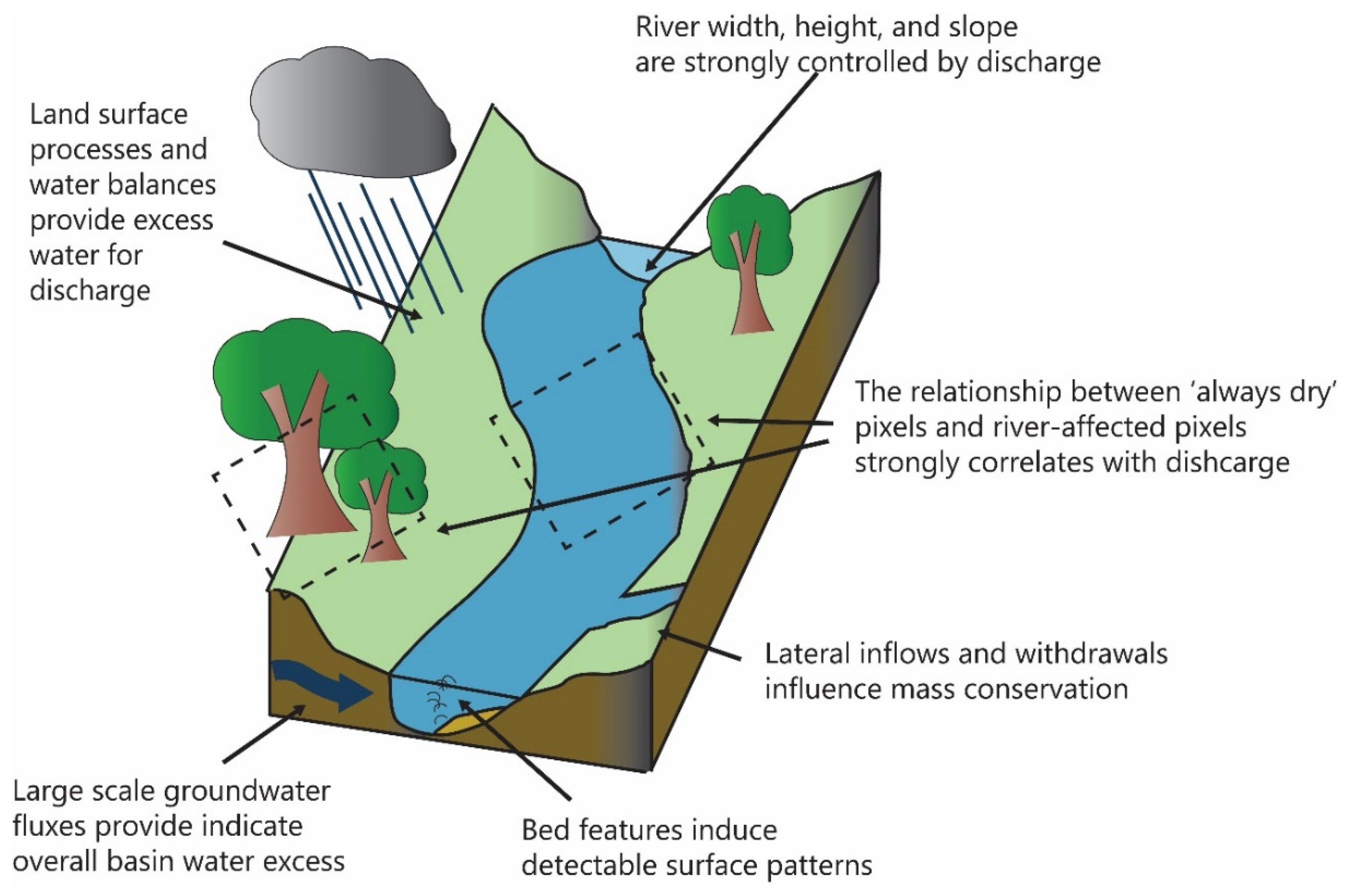
Whatever the RS signal, the idea that RS observations correlate with discharge is powerful. This can move the idea of a rating curve beyond measuring channel stage and/or width toward measuring other targets that can reliably drive RSQ. The work pioneered by Brakenridge et al. ([89]; 2007) illustrates this concept excellently. In this 2007 paper, building off their previous work, Brakenridge et al. identify a simple and powerful phenomenon. They observed that the response of passive microwave satellite observations of river channels relative to a nearby ‘dry’ land area (what they call the ratio between a calibration area C and measurement area M) is strongly correlated with river discharge. The logic behind the Brakenridge ratio is that rivers get wider as discharge increases (the same as the width-based rating curves noted above), but it is not necessary to precisely quantify this top width change (see Figure 3). Rivers do indeed get wider with discharge, but soil moisture near the river also increases and there are numerous spatial changes to the river surface not captured by cross sectional top width changes. A ‘wet’ pixel thus reflects quantities changing with discharge, even if it does not track changes in width directly, while the nearby ‘dry’ pixel is relatively insensitive to these changes. Using a ratio between wet and dry allows a finer response to hydrologic forcing than tracking uncalibrated changes to the ‘wet’ area alone. Further, this approach has the advantage of spatial resolution—coarser ground areas may be considered rather than precise measurements of river width, thus overcoming errors in discharge that propagate from width measurement errors. With this ratio in hand, Brakenridge et al. made rating curves from in situ discharges using higher order polynomial regression.

Since this 2007 publication, this ratio approach has grown into a successful subfield of RSQ that was born from the unique hydrologic vantage point of RS, unlike space based rating curves, which are extensions of ground hydrology. The McFLI approaches covered in Section 2.2.2 are similarly fundamentally tied to a RS vantage point, and both of these ‘schools’ of RSQ are conceived with RS data in mind from the onset. In 2012, Brakenridge et al. [90] pushed their approach to thousands of global stations, using a previously in-situ calibrated hydrology model to provide the training data for discharge predictions. In this case the model provides ‘truth’ to guide the remote sensing, so applicability of this method is dependent on faith in the model output, and in this we see a strong parallel with the studies of Section 2.1.1. Tarpanelli et al. [91]; 2013) proved the same ratio concept is viable from visible and near-infrared observations, and Van Dijk et al. ([92]; 2016) investigated the global potential for the ratio approach while explicitly considering tradeoffs between passive and active sensors. Tarpanelli et al. have led efforts to refine this approach, with papers in 2017 [93] and 2018 [94] that consider fusion between optical imagery and altimetry while also investigating machine learning (rather than regression) for training algorithms. This work also branches toward the spatial extension of training data through hydrologic modelling, which moves this application squarely beyond well- and semi-gauged basins and into regionally gauged basins.

In Pursuit of Local Channel Hydraulic Parameters

A final channel hydraulic calibration was recognized by scientists as early as the 1970s, when Lynzenga ([95]; 1978) calibrated the reflectance of the bottom of a water column to field measurements to yield a remotely sensed estimate of depth. The principle behind remote sensing of depth is driven by attenuation of light in a water column (Beer’s Law). Lee et al. ([96,97]; 1998; 1999) describe this process for vertically homogenous, optically shallow waters (i.e., water columns in which light is able to reflect from the channel bottom and back through the water surface). They separated observed upwelling radiance into three parts—bottom reflectance, surface reflectance, and air column radiance, while controlling for water column attenuation. Lee et al. noted that slight changes in turbidity affect the performance of depth retrieval, so the model must be parameterized according to the properties of the water in both space and time, making this approach impractical in a global sense. Contemporary work continued in this vein (e.g., [98]; Gould et al., 1999), until Fonstad and Marcus ([99]; 2005) and Marcus and Fonstad ([100]; 2008) were among the first to translate this approach to rivers. Remote sensing scientist Carl Legleiter has built on this heritage with a calibrated approach termed optical band ratio analysis (OBRA), first published in 2009 [101]. This approach is built on the same principles of reflection and attenuation as earlier work, and requires calibration or assumption of optical properties to back out river depth. This OBRA approach has been successfully demonstrated in numerous contexts ([102,103,104]; Legleiter, 2015; Legleiter et al., 2017; Smith et al., 2015). Alternatively, Johnson and Cowen ([105]; 2016) used highly controlled flume experiments to provide estimates of bathymetry based on observed turbulence structures. For example, riffles or hydraulic jumps on a water surface are indications of changes in channel structure. In all cases, these observations need be calibrated with some in situ information to yield discharge.

If calibrated optical attenuation and other approaches can be used to provide depth estimates, then only channel velocity is needed for a discharge estimate. Costa et al. ([106]; 2000) provide an early remote sensing of velocity method, but this approach requires sophisticated equipment, highly trained personnel, and a bridge: it is not a practical approach for numerous rivers. Further, surface velocity is not the same as the depth-averaged velocity needed to estimate discharge, and more reductive assumptions are needed to transform one to the other. However, Costa et al. provide a proof of concept for remote sensing of channel velocity. More recent work has focused on two basic techniques: Particle Image Velocimetry (tracking particles on water surfaces using image processing techniques) and leveraging turbulence structures. Legleiter et al. ([103]; 2017), for instance, used the OBRA technique for river depth and bridge-based thermal imagery to track surface velocity. A number of recent papers flesh this out, in the context of applying entropy theory to the cross-sectional velocity profile ([107,108,109,110]; Chiu, 1991; Fulton and Ostrowski, 2008; Moramarco et al., 2017; 2019). All of these investigations are aided by better geomorphic knowledge of channels, and RS can be useful here too, often through lidar mapping of topography and sometimes bathymetry (e.g., [111]; Hilldale and Raff, 2008). These and the other papers in Section 2.1 show that highly accurate discharge can be estimated from RS, and there seems to be a tradeoff in discharge accuracy vs. the amount of prior data we have on a river, making the most accurate RSQ estimates in the best-understood basins.

2.2. Politcally and Totally Ungauged Basins

Fundamentally, RSQ in ungauged basins is an ill posed problem. We cannot measure enough hydraulics from RS to solve for discharge directly, as bathymetry, friction, and discharge will always be unknown in a channel without calibration. The approaches in Section 2.1 might use reasonable values for friction based on knowledge of the basin/channels, or pull bathymetry from a regional regression, or use a hydrologic model, or bypass the hydraulics and calibrate discharge directly to a RS signal to circumvent this problem. The approaches in Section 2.2, however, seek to overcome the problem solely from outer space, limiting themselves to assumptions about rivers that may be made only from RS data or other global data that are independent of specific calibration. The accuracy of these approaches tends to be much lower than the approaches in Section 2.1, yet as we note in Figure 1 the goal of these authors is to improve on what we know in ungauged basins. Given that in many ungauged basins we know very little, even approaches with high errors in discharge can be useful. This literature is much smaller than the scholarly output for Section 2.1, and as such we cover this literature in slightly more depth.

2.2.1. Calibration/Assimilation of an RS Signal into a Hydrologic Model

We first consider RSQ as seen again from a hydrologic perspective, yet this time we focus on RS as the sole source of calibration data, as opposed to use of RS data in conjunction with an in situ calibrated model as in Section 2.1. The balance of these fluxes is water excess, and so a valid RSQ approach is to emulate a hydrologic model solely from outer space. Various authors have investigated RS of each of these specific components in an effort to better constrain each one. Parr et al. ([112]; 2015) used RS ET and leaf area index products in conjunction with the VIC model, while Lopez-Lopez et al. ([113]; 2018) explored downscaling and in 2017 calibrated the PCR GLOBWB model for a basin in Morocco with RS ET and soil moisture, and both concluded that their approach is viable and improves discharge accuracy [114]. However, Mendiguren et al. ([115]; 2017) and Bowman et al. ([116]; 2016) explicitly compared RS ET energy balance models against traditionally calibrated hydrological models and found low correlation between the two products. These authors further argued that the spatial component of errors in ET are important and well-suited to remote sensing. Remote sensing of precipitation is a huge field given the importance of precipitation to flood forecasting, and thus this literature is not covered here despite providing important grounding and uncertainty analysis to RSQ; see Lettenmaier et al. ([2]; 2015) for a recent review. While this precipitation literature is certainly germane, any satisfactory review would render this manuscript overlong. The GRACE signals covered in Section 2.1.1 can provide the final storage term, and thus a simple water balance may be made at very large spatial footprints for totally and politically ungauged basins from RS estimates of precipitation, ET, and storage.

Moving beyond a simple water balance, Sun et al. ([117]; 2015) provide a basin-scale approach that seeks to use no in situ data to calibrate their hydrologic model, instead using river width observations as a calibration target. This decision required a reconfiguration of traditional model physics to represent width as the state variable (i.e., rearranging the discharge equation so width is on the left hand side). Sun et al. then attempt to force their hydrology model with only globally available data, using the dynamic river width signal to calibrate. Emery et al. ([118]; 2018) follow Brakenridge et al. ([90]; 2012) in using a hydrologic model ‘off the shelf’ to provide calibration data, where their calibrating model was itself previously calibrated using altimetry to track water levels ([82]; Paris et al. 2016). Emery et al. then use this RS-driven model and new, independent altimetry estimates of river stage as inputs to a second hydrologic model, tuning the model based on the Paris et al. ([82]; 2016) discharges. In this approach we see the coupling of the work in Section 2.1.1 and Section 2.1.3: using RS signals for both hydraulic and hydrologic components. We have placed this work in the ‘ungauged’ category. On the one hand, Sun et al. and Emery et al. needed no in situ data in their specific approaches and can rightly claim their techniques work in ungauged basins. However, their forcing data, while uniformly available, relied on in situ calibration data from either precipitation gauges or stream gauges in the US and Europe (Sun et al.), or from a specific region (Emery et al.). This idea can be taken further in the context of the Lin et al. ([14]; 2019) paper discussed earlier: that study used over 10,000 in situ gauges to produce the best possible global discharge estimates at almost 3 million river reaches. These Lin et al. data are globally available and consistent, and offer a starting point for any model assimilation/calibration study, be it hydrologic, hydraulic, or both. However, using these outputs necessarily invokes the gauges used to produce them: even discharge information in gauge-sparse locations like Siberia implicitly relies on gauge knowledge via coupling with well-gauged basins. Thus, we expect future work to struggle with what it means for a basin to be ungauged when all global basins have been modelled in a fully coupled land surface framework. We leave further discussion for Section 3.

2.2.2. Assimilation/Calibration of an RS Signal into a Hydraulic Model

RS signals can also be incorporated into models that explicitly represent some aspect of channel hydraulics without in situ data, just as in Section 2.1.2. These representations of hydraulics could range from a full computational fluid dynamics finite element model solving for full four dimensional conservation of energy, mass, and momentum in time, to simple box-channel routing models capable of reproducing channel stage but not width, to Manning’s equation. This channel-based paradigm is perhaps more familiar to readers, as two of the river variables with the longest remote sensing heritage, width and stage, are often employed in these approaches. Bates et al. ([119]; 1997) summarized early work on RS and flood hydraulic modelling, noting the sharp change in fluvial behavior once a river enters its floodplain. Bates et al. noted that computationally efficient one-dimensional flow modelling is acceptable within bank, but not in overbank situations, but also argued that RS signals are ideally poised to capture actual flood events (also noted by [120]; Brakenridge et al., 1998). Thus, RS is well suited to locations where traditional one-dimensional hydraulic models poorly represent hydraulics. Bates et al. conclude by noting that floodplains in particular are excellently suited to RS, as when they are dry, they may be mapped and their elevations recorded for future flood models (furthered in nuance by [121,122,123]; Horritt and Bates, 2001, Poole et al., 2002, and Horritt, 2006). Then, RS can capture actual floodwater occupation of the floodplain area and transform this into floodplain water depth in order to calibrate the model. Following these early works, many examples of calibration of hydraulic models with RS information have since focused on a flooding context (e.g., [63,124,125,126,127,128,129,130,131], Gumley and King, 1995; Mason et al., 2007; Schumann et al., 2007; 2008; 2009; Coe et al., 2008, Di Baldassarre et al., 2009; Khan et al., 2011; Frasson et al., 2019). Some of these studies assume upstream flow is known and then use RS to improve downstream flow, but it is possible to iteratively force a model with different flows and an explicit hydraulic model until model output matches RS observations in the floodplain, as Sun et al. did with width in Section 2.2.1. Thus, here we see calibration of a model to RS data, rather than calibrating RS data to a gauge or a model as in Section 2.1.

More recently, advances in global mapping, computational power, and the lengthening of the satellite data record has made a quantum leap in the amount of RS signals available for calibration of hydraulic models. Consider the Pekel et al. ([11]; 2016) product, which classified every single Landsat image in the archive into areas of water and non-water, allowing researchers to track global changes in inundation dynamics and river surface areas (i.e., width) directly for a 32 year period. Using the logic of Bates et al. ([119,132]; 1997; 2003), these changes in surface area can reveal flood stage extents and even heights when mapped onto newly available DEMs built for hydrology (e.g., MERIT DEM, [10] Yamazaki 2019). These inundation signals can also be obtained from non-optical satellites (e.g., [133]; Du et al., 2018), or even from non-satellites (e.g., UAVs, [134]; Niedzielski et al., 2016). As the satellite archive grows, and especially if new commercial CubeSats continue to improve their radiometric calibration and geolocation errors, we predict that approaches built on assimilating/calibrating these signals will proliferate.

Some of this proliferation is underway and is potentially overcoming reliance on gauges we see in the work of the late 2000s. Sichangi et al. ([23]; 2016) offer an interesting approach coupling altimetry, MODIS, and a DEM for eight very large rivers globally. They assume a wide channel with a constant width (greatly simplifying hydraulics), which allows a set of hydraulic equations to be driven by altimetry, which they calibrated with the nearest available altimetry gauge station. This rightly places this paper in Section 2.1.3, but this example shows that the field is moving toward consciously focusing on attempting to eliminate the need for in situ data, presumably to better understand ungauged basins in future.

Andreadis et al. ([135]; 2007) and Durand et al. ([136]; 2008) laid groundwork for RSQ from hydraulic models without any in situ data or global model inputs via detailed experiments to understand how well data assimilation was able to reproduce unknown channel parameters (e.g., friction, bathymetry, flow) from synthetic RS measurements of channel width, slope, and height within a simple hydraulic model. Biancamaria et al. [137]; 2011) and Yoon et al. ([138]; 2012) performed the next generation of this work, which lead to ‘4D’ variational data assimilation (VDA) within an uncalibrated hydraulic model ([139,140,141,142]; Gejadze and Malaterre, 2017; Oubanas et al. 2018a; b; Larnier et al., 2020), and these recent efforts offer the most sophisticated take on this problem. This computationally expensive approach is able to consider model states both forward and backward in time and consider uncertainties of both initial model expectations and RS data. 4D VDA considers that initial flow is a static hydrograph, thus removing a dependency on external hydrologic modelling. These authors have shown that accurate discharges can be estimated using this approach, and that these approaches are viable indeed in politically and totally ungauged basins, but sensitivity to the initial hydrograph and computational burden are challenges for large-area application.

2.2.3. Geomorphic Inverse Problems

Finally, we consider approaches to RSQ that again independently consider hydraulic components of discharge (as in Section 2.1.3), but here explicitly rely on geomorphology, RS, and global databases. These approaches are driven by many of the same geomorphic hydraulic models of Section 2.1.2. A special case of geomorphically driven inverse problems is the mass conserved flow law inversion (McFLI) approach. Gleason et al. ([25]; 2017) coined the term as a response to a growing body of the RSQ literature that made the same basic assumptions about how to approach RSQ. Many of these approaches were motivated by the upcoming surface water and ocean topography (SWOT) mission as authors thought about how to best to use SWOT’s novel and simultaneous measurements of river width, height, and slope, but McFLI approaches are fundamentally independent from SWOT. Durand et al. ([143]; 2010) laid the groundwork for McFLI with a mathematical approach that required known friction coefficients a priori, but the first true examples of McFLI capable of working in totally ungauged basins without this restrictive assumption were all published in 2014 or 2015. In a McFLI approach, authors first assume that a set of cross sections in a reach, or alternatively a set of short connected reaches, are mass conserved. What remains is to solve for unknown parameters in a flow law (e.g., Manning’s, hydraulic geometry) given RS observations, meaning the problem remains ill-posed but is now more constrained and solutions may be approximated exclusively from remotely sensed data. Like the ratio approach pioneered by Brakenridge et al. ([89]; 2007), McFLI approaches are fundamentally a product of a remotely sensed paradigm. To a McFLI, a remotely sensed snapshot of a river is just that—a moment frozen in time capturing data over a large spatial area. Traditional geomorphology tends to consider evolution of rivers at a single point over long time periods or considers geologically synoptic spatial patterns. McFLI considers the temporal co-evolution of interconnected fluvial entities, which matches RS observations perfectly.

Both Garambois and Monnier ([144]; 2015) and Durand et al. ([145]; 2014) published McFLI algorithms based on Manning’s equation assuming known (vis RS) river surface elevation, width, and slope. Unknown parameters are thus Manning’s n, some unobserved area below the lowest water surface elevation observation, and discharge. We must note that these data are currently not available from RS without painstaking fusion of optical and altimetry datasets confounded by cloud issues and orbit geometry. Bjerklie et al. ([146]; 2018) were able to produce such signals for one river in Alaska, but most Manning’s based McFLI approaches use model data to simulate RS measurements. Durand et al. used these simulated data to solve this problem in a Bayesian context by using likelihood functions in a Markov chain to allow estimates of these unobserved parameters to converge toward a likely posterior distribution. Tuozzolo et al. ([147]; 2019) have explored the impact of reach vs cross section based formulations of Manning’s equation for this purpose. Garambois and Monnier used an optimization algorithm to define the pareto parameters that best minimized errors given a set of constraints (including mass conservation) for the same simulated data. Moving toward real data, Altenau et al. ([148]; 2017) showed that SWOT’s Ka-Band observations should function as intended, using an airborne Ka-band radar to produce the same observations as SWOT, and Tuozzolo et al. ([149]; 2019) were able to use these airborne observations to successfully give first demonstration of a Manning based McFLI from wide swath altimetry.

Manning’s equation is not the only Flow Law invoked in McFLI. Gleason et al. ([24,150]; 2014a;b) proposed a McFLI based on hydraulic geometry (both at a station and at many stations), which requires only river width as an observable input. Unknown parameters in this McFLI are the width exponent of the hydraulic geometry power law and two at many stations’ hydraulic geometry constants specific to each river. This width-based McFLI has been successfully demonstrated for Landsat, Sentinel, and Planet optical imagery ([24,84,151]; Gleason and Smith, 2014; Gleason et al., 2014; Gleason and Hamdan, 2015; Feng et al., 2019), first using a genetic algorithm to solve for discharge and later using a Bayesian formulation capable of width-only or width, height, and slope discharge inversion ([152]; Hagemann et al., 2016). Currently, this width-based McFLI is the only known technique capable of leveraging existing satellite data to run a McFLI at all totally ungauged basins at the global scale given our definitions here.

Both Bonnema et al. ([153]; 2016) and Durand et al. ([154]; 2016) have intercompared McFLI approaches using a variety of hydraulic model data to stand in for remotely sensed observations. Durand et al. in particular provided the first ever exhaustive comparison of multiple McFLI approaches on model output representing almost 20 rivers. This controlled experiment allowed Durand et al. to more deeply understand controls on error and accuracy in McFLI approaches. They concluded that approaches that use multiple inputs (i.e., width, height, and slope) generally outperform approaches that use only a single input (i.e., width alone), as expected. They also concluded that all McFLI approaches provide good estimates of discharge dynamics, but all frequently have large biases. These biases are difficult to overcome without better prior estimates of unknown parameters because of the equifinal nature of McFLI. Finally, Durand et al. found that methods are sensitive to prior expectations of unknown parameters (either the ‘first guess’ in an optimization problem or the Bayesian ‘prior distribution’), but that all methods improve upon these priors. That is, McFLI methods estimate discharge on rivers more accurately than our initial estimate of discharge without in situ or calibration data of any kind, but the more we know about a river to start with, the better the final estimate of discharge will be. This point becomes a critical determinant in choosing an RSQ method in the context of Figure 1 and Figure 4.

Sichangi et al., ([155]; 2018) offer a different take on underconstrained geomorphic inversion. They used MODIS to back out the travel time of a flood wave by looking at the peak of a width signal at multiple stations in a MODIS river width-time plot. That is, they assumed that maximum widths at any cross section correspond to maximum discharge (a safe assumption per hydraulic geometry) and that the peaks in both stations correspond to the same hydrologic event. Thus, two stations 500 km apart yielded a bulk channel velocity (travel time) by tracking the time delay between width peaks at the two stations. This is an innovative and clever approach to sensing channel velocity from space, but did require Sichangi et al. to assume a Manning’s n from look up tables of values ([156]; Chow, 1964) to back out channel depth, and relies on a conversion from celerity to velocity. This rather exciting idea is only useful on large rivers where bulk velocity is stable over long distances and where the assumption of a travelling maximum width is valid. This again also highlights how not all ungauged approaches are applicable globally, and how some assumptions are considered restrictive and others are not. If, for instance, an author can study imagery of a river and a global DEM to determine probable Rosgen ([157]; 1994) classes, then assumptions about friction and width/depth ratios, for example, are well founded and did not invoke in situ data.

3. Discussion

Our broad sketch of the literature has hopefully revealed the numerous ways hydrologists have approached RSQ. We have deliberately included as wide a swath of the literature as possible to fully contextualize the field for practitioners and other interested parties alike. We have raised several discussion points above without bringing them to conclusion, saving them instead for this present section. Specifically, we wish to further probe several ideas that render even our nuanced classification of what it means to be ‘gauged’ or ‘ungauged’ problematic vis a vis RSQ; we wish to address common misconceptions about RSQ; and finally we wish to consider human political and economic realities of RSQ.

3.1. A Framework for Understanding RSQ, Ungauged Basins, and Hydrologic Knowledge

Although we did not keep a tally, a majority of the literature surveyed mentioned ungauged basins in their introduction as a justification for the work. We have thus used our gauge continuum to explicitly parse the literature at this highest level, placing each study into our understanding of the appropriate context. However, we have repeatedly raised the question of what it means to be ungauged in an era of global hydrologic modelling. Traditionally, RSQ authors have argued only those studies invoking absolutely no in situ data whatsoever qualify as appropriate for ungauged. RSQ via regionalization (parameter transfer) thus fails this test, and so too does parameterization from a global or regional model as there are almost no global hydrology datasets available that do not invoke in situ calibration data. Even the most basic RS water balance relies on precipitation gauges to calibrate the precipitation signal—without it, these estimates would likely be so wildly wrong as to be not useable. While we maintain an explicit difference between regionalization/ regional calibration vs. coupled modelling, we recognize that global hydrology has advanced tremendously in the RSQ era and thus believe that any RSQ investigation in an ungauged basin will (and should) likely start from an off the shelf global hydrology model to provide a first guess or Bayesian prior. Therefore, following our survey of the literature, we propose the following four conditions for when an RSQ approach is truly capable of tackling totally or politically ungauged basins.

In order to be applicable in totally and politically ungauged basins:

• The study uses only globally available hydrologic (e.g., P, ET, runoff) forcing
• If a global model is used, the study must not calibrate an RS signal explicitly to it
• The study does not transfer parameters or calibrate to regionally available gauges
• Specific assumptions about channel hydraulics must be obtained exclusively from remotely sensed platforms

These tests should be applied to each new ungauged study to ensure that the primary RS data is indeed driving the discharge result, rather than in situ data available elsewhere. We argue that this independence is essential for politically and totally ungauged basins, as otherwise reviewers and the public will rightly question whether or not discharges in these basins are simply a regurgitation of what we knew before. Hence, we believe that if basins are truly ungauged, models can only guide or bound RSQ, not drive it. Applying these restrictions could limit the accuracy of the resulting discharges ([144,154]; Garambois and Monnier, 2014; Durand et al., 2016), but we argue that these less accurate but independent discharges represent the largest furthering of hydrologic knowledge in these cases and allow hydrologists to make declarative statements about the water cycle.

This is not to say that studies that do not meet these criteria are not RSQ: on the contrary, the vast majority of the literature surveyed here is uninterested entirely with meeting these criteria. Rather, we introduce these tests as a useful filter for future reviewers and authors to help decide what technique is best for a particular application. Thus, RSQ methods need not change if these tests are failed, rather, their introduction should highlight the context of regionally or locally available information and place the study into the appropriate category. Our emphasis on avoiding transferability is grounded in field hydrology, as we, like McDonnel et al. ([12]; 2007), are wary of assuming hydrologic process in unknown and unstudied watersheds. For example, using gauges from one watershed to calibrate a fully coupled earth system model at the continental scale is, to us, fundamentally different than assuming the parameters calibrated for that one watershed should apply to all basins across the continent. The lines between ‘regionally gauged’ and ‘totally ungauged’ are becoming blurred as coupled earth system models produce fluxes with greater accuracy and precision. Even so, we maintain a fundamental difference between using a global hydrology product as a starting point for an RSQ method vs. calibrating an RS signal to that model to produce discharge. In the latter, the resulting discharges are fundamentally a product of the original model: at best, RSQ would give you the model discharge back again. In this case, RS would be better used in conjunction with other data to produce the global product in a hydrologic model as in Section 2.1.1, rather than exist as a derived product. Finally, we assert that while in situ data are important to improve the accuracy of RSQ, they are not indispensable. The breadth of the literature covered here makes this abundantly clear, and we see value in pursuing RSQ research across the entire gauge spectrum.

We believe that review of the myriad of techniques for RSQ herein is secondary to definition of the paradigm in which they are employed. While methodological innovation is essential, the literature has revealed that the more data an author has in hand to begin an RSQ study, the more accurate their final discharges. While we have very purposefully avoided the tedium of reporting individual discharge retrieval accuracies across the literature given the impossibility of direct comparison following specific sets of assumptions, RS data, and ancillary data used in each case, we can assert in general that the literature in Section 2.1 is more accurate than the literature in Section 2.2. This is of course intuitive—studies in Section 2.1 all used local or regional gauge data or tailored assumptions of hydraulics specifically to study channels given prior knowledge. However, the methods of Section 2.2 can perform as accurately as those of Section 2.1 given the same calibration data ((141,144); Garambois and Monnier, 2015; Oubanas et al., 2018). Thus, we have chosen to organize the literature by application area first and methodology second, as differences in accuracy are driven largely by prior data and not methodology. Nowhere have we split the literature via sensor, as we find papers arguing for or against specific sensing platforms at the cost of others unhelpful. We do recognize the advantages of passive/active sensors at varying resolutions for specific tasks, but argue that ultimately what matters is whether or not the study has achieved its goal. Figure 3 exists in service of this goal, highlighting all the usable RS signals we have reviewed here in a single figure.

At its core, RSQ seeks to advance hydrologic understanding. In basins that are gauged, semi-gauged, or regionally gauged, hydrologists start with some of this understanding in hand, and RSQ should improve our ability to parse the hydrologic cycle in space and time. For water resource managers, even a well-gauged basin can have insufficient understanding when attempting to balance hydropower, environmental flows, drought/flood protection, and recreational use ([158]; Brown et al., 2015). RSQ can thus provide real advances in hydrologic understanding that improve human decision making, even in gauged basins. In politically and totally ungauged basins, we suggest that methods that produce hydrographs in error by even a factor of two or more (although we must rely on their performance in gauged basins to characterize this error) might still be an improvement on our existing knowledge. Therefore, we assert that nearly all RSQ is useful to the hydrology community provided authors place their study in the proper context. This context, given here and in Figure 1, is essential for practitioners, authors, reviewers, and editors. Without it, non RS hydrologists can be confused as to whether or not a given technique will work for their application, and editors and reviewers may accept otherwise excellent RSQ work that makes claims of being “ungauged” that it cannot support.

3.2. “The Goal of Remote Sensing of Discharge is to Entirely Replace Gauges”: A Common Misconception

RSQ is designed to produce river discharge and the advantages of air and spaceborne platforms over grueling fieldwork are clear and much touted by RSQ authors. This might lead some to believe that a goal of RSQ is to replace expensive and politically sensitive gauge data. Thus, this section title represents a pernicious misconception about RSQ. The majority of the work cited above requires gauges to produce successful discharge estimates, and even those methods in Section 2.2 that do not require gauge data improve dramatically when informed by gauge data. There will never be any hydrologic substitute for gauge data—these data are carefully monitored by dedicated staff of numerous agencies worldwide, and many agencies go to great lengths to ensure that only the highest quality data are presented as the gauge record. This can have political consequences, as many gauge data receive the ‘seal of approval’ of officially sanctioned government agencies, and a hydrologic world without sanctioned discharges would place much of climate science and water treaties in jeopardy. With that stated, there has been a precipitous decline in available gauge data globally ([159]; Hannah, 2011), and public gauge records are practically nonexistent in places where water politics are thorny ([151]; Gleason and Hamdan, 2015). Gauges that are here today may be gone tomorrow at the whims of economics and politics.

Thus, we believe that RSQ is a natural complement to river gauges and other in situ discharge monitoring. In this we agree with Fekete et al. ([160]; 2012), even if we have drawn this conclusion via very different means. The benefits of in situ data to RSQ are clear and have been discussed extensively above. Here, we discuss the benefits of RS signals to in situ monitoring. Consider a well-gauged river network, with a gauge at the outlet and across a large proportion of ungauged upstream reaches. RSQ may actually be at its most beneficial in this case, as high quality gauge calibration data allow RS signals to extend point gauge measurements in space and time. As networks move along the continuum from completely gauged to ungauged, RSQ provides more novel primary information, but RSQ retrievals reduce in accuracy. Alsdorf et al. ([22]; 2007) also highlight that RSQ can document water resources in diverse channel forms and in flood contexts: situations where gauges struggle. Discontinued gauges are another area where RSQ can shine, as gauges that overlap the RS record in the past can be calibrated and then used to parameterize models as they move into the future (e.g., [161,162]; Birkinshaw et al., 2010; Gleason et al., 2018).

In sum, we argue that no RSQ practitioner can or should cogently argue that RSQ is a complete replacement for gauges. Both forms of discharge monitoring have strengths and it is only by merging the two that hydrology can move forward toward more complete understanding of the global hydrologic cycle. The Arctic and much of Asia are almost complete hydrologic black boxes, despite the almost certain existence of un-shared high quality gauge data in these places. Lin et al. ([14]; 2019) highlight the benefits of even sparse global gauging by considering a coupled land-atmosphere system, primary data with low uncertainty might be used to reduce uncertainty in poorly monitored areas, and in this case RS data provide a welcome and irreplaceable source of primary data. We believe that hydrology, like many geophysical disciplines, should rest on primary data, and loss of either gauge or remotely sensed data is a detriment to the field.

3.3. Ethics and Politics

Finally, we wish to make a brief note on the ethics and politics of RSQ. Gleason and Hamdan ([151]; 2016) and Alvarez-Leon and Gleason ([163]; 2017) have recently explored this topic and have concluded that RSQ is an inherently political act. They reached this conclusion following two different logical tacks. First, since states (the preferred term for ‘country’ in the geographical literature) own their water resources, they are allowed to express their national sovereignty by withholding hydrometric data (i.e., politically ungauged basins). There is no international legal mechanism to force states to release water data, and even bi- or multi-lateral treaties have proven ineffective at forcing water data transparency, despite assertations that such transparency is essential for good governance ([164,165,166,167,168]; Sneddon and Fox, 2006; 2011; 2012; Dore and Lebel, 2010; Ho, 2014). Circumventing these data restrictions via the use of satellites is thus in fact a direct violation of national sovereignty and an inherently political act, regardless of the intent of the scientist ([151] Gleason and Hamdan, 2016). This is not to say that practitioners should not engage in RSQ—on the contrary, there are humanitarian and climate reasons why scientists should perform this very political act. However, scientists have no recourse to state that they are ‘simply observing the earth’ are thus somehow immune to politics. This is a naïve view that has long been debunked in social sciences and the humanities, but is slow to catch on in the non-social sciences, especially in remote sensing. Second, access to satellite data themselves is a result of political decisions ([163] Alvarez-Leon and Gleason, 2017). The United States government has launched a fleet of earth observing satellites, and made it their policy that all of these data are available to anyone with access to the internet. Despite this, the United States government could change its mind at any point and restrict access to these data, thus blanketing access to these crucial primary data in an instant. We do not suggest this is a likely scenario, but it is possible. Consider the numerous other commercial and state-satellites that exist but for whom data are not free or simply not available outside of the home state. Public access to high quality earth system data is ultimately subject to the whims of the owners of the satellites themselves, and this access has profound impacts on hydrologists’ ability to perform RSQ. Taken together, these two arguments suggest that practitioners should take care and make thoughtful choices when applying RSQ in contexts where it would be politically impossible to gather the same data in the field. This forms a good test, and ‘Would I have permission to do this RS work as fieldwork?’ should be a question practitioners ask themselves when beginning a study. If the answer is ‘no,’ practitioners should proceed if believe it is appropriate, but they should be aware of the implications of the study.

4. Conclusions

The existing RSQ literature has frequently justified itself based on whether it is highly accurate or whether it is applicable in ungauged basins. Each new manuscript generally begins with an explicit statement on the utility of RSQ and why this new work belongs in the pantheon of that particular application, yet much work claiming to function in ungauged basins often cannot, by our definitions, truly work in ungauged basins. This leads to evident division in citations within RSQ studies—authors typically only cite work within the categories (i.e., sections and subsections) presented here, and papers frequently do not incorporate information from different ‘families’ of RSQ. What we have shown, however, is that many of these seemingly disparate methods are in fact slight variations on the same paradigm, and that the entirety of the literature has more in common than individual papers would suggest. Our inclusion of ‘non channel’ RSQ here is perhaps controversial to some along this vein, as many RSQ practitioners might suggest that using RS signals within a hydrologic model is somehow not RSQ. It is our hope that this review serves as a reminder that in all cases reviewed here, remotely sensed data were used to estimate discharge in service of furthering discharge understanding. There are nuances in how this was achieved, but all ~170 papers here have the same goal. Finally, we suggest that our newly defined framing for application of RSQ (e.g., Figure 1 and Section 3.1, Figure 4) might offer much clarity to readers, authors, editors, reviewers, and importantly users of RSQ.

Our review has also implicitly outlined some future directions for the field, which we make explicit here. Data mining/big data approaches seem particularly understudied despite the success of Bjerklie in the early 2000s, and the availability of powerful computer science techniques available to hydrologists today makes this area ripe for potential powerful interventions in RSQ. Satellites dedicated to surface water and sponsored by large state entities (like SWOT), and commercial fleets of CubeSats alike also stand to transform the field. While SWOT has received much attention in the literature from many schools of RSQ, CubeSats are relatively underused. Diverse signals can only improve what we know about the hydrologic system. Finally, we repeat our call for a broadening of perspective of RSQ practitioners. We have shown here that the field is robust, rapidly growing, and rich with an extraordinary diversity of ideas. The field would suffer, we believe, from a descent into orthodoxy, which might stifle creativity. Instead, we hope that new works can use this review as a basis to situate their work in broader context.

References

- Calmant, S.; Seyler, F.; Cretaux, J.F. Monitoring Continental Surface Waters by Satellite Altimetry. Surv. Geophys. 2008, 29, 247–269. [Google Scholar] [CrossRef]
- Lettenmaier, D.P.; Alsdorf, D.; Dozier, J.; Huffman, G.J.; Pan, M.; Wood, E.F. Inroads of remote sensing into hydrologic science during the WRR era. Water Resour. Res. 2015, 51, 7309–7342. [Google Scholar] [CrossRef]
- Doell, P.; Douville, H.; Guentner, A.; Mueller Schmied, H.; Wada, Y. Modelling Freshwater Resources at the Global Scale: Challenges and Prospects. Surv. Geophys. 2016, 37, 195–221. [Google Scholar] [CrossRef] [Green Version]
- Lettenmaier, D.P.; Famiglietti, J.S. Hydrology—Water from on high. Nature 2006, 444, 562–563. [Google Scholar] [CrossRef]
- Allen, G.H.; Pavelsky, T.M.; Barefoot, E.A.; Lamb, M.P.; Butman, D.; Tashie, A.; Gleason, C.J. Similarity of stream width distributions across headwater systems. Nat. Commun. 2018, 9, 610. [Google Scholar] [CrossRef]
- Smith, L.C.; Yang, K.; Pitcher, L.H.; Overstreet, B.T.; Chu, V.W.; Rennermalm, Å.K.; Ryan, J.C.; Cooper, M.G.; Gleason, C.J.; Tedesco, M.; et al. Direct measurements of meltwater runoff on the Greenland ice sheet surface. Proc. Natl. Acad. Sci. USA 2017, 114, E10622–E10631. [Google Scholar] [CrossRef] [Green Version]
- Lehner, B.; Döll, P. Development and validation of a global database of lakes, reservoirs and wetlands. J. Hydrol. 2004, 296, 1–22. [Google Scholar] [CrossRef]
- Prigent, C.; Matthews, E.; Aires, F.; Rossow, W.B. Remote sensing of global wetland dynamics with multiple satellite data sets. Geophys. Res. Lett. 2001, 28, 4631–4634. [Google Scholar] [CrossRef] [Green Version]
- Allen, G.H.; Pavelsky, T.M. Patterns of river width and surface area revealed by the satellite-derived North American River Width data set. Geophys. Res. Lett. 2015, 42, 395–402. [Google Scholar] [CrossRef]
- Yamazaki, D.; Ikeshima, D.; Sosa, J.; Bates, P.D.; Allen, G.H.; Pavelsky, T.M. MERIT Hydro: A High-Resolution Global Hydrography Map Based on Latest Topography Dataset. Water Resour. Res. 2019, 55, 5053–5073. [Google Scholar] [CrossRef] [Green Version]
- Pekel, J.-F.; Cottam, A.; Gorelick, N.; Belward, A.S. High-resolution mapping of global surface water and its long-term changes. Nature 2016, 540, 418–422. [Google Scholar] [CrossRef] [PubMed]
- McDonnell, J.J.; Sivapalan, M.; Vaché, K.; Dunn, S.; Grant, G.; Haggerty, R.; Hinz, C.; Hooper, R.; Kirchner, J.; Roderick, M.L.; et al. Moving beyond heterogeneity and process complexity: A new vision for watershed hydrology. Water Resour. Res. 2007, 43. [Google Scholar] [CrossRef] [Green Version]
- Wood, E.F.; Roundy, J.K.; Troy, T.J.; van Beek, L.P.H.; Bierkens, M.F.P.; Blyth, E.; de Roo, A.; Döll, P.; Ek, M.; Famiglietti, J.; et al. Hyperresolution global land surface modeling: Meeting a grand challenge for monitoring Earth’s terrestrial water. Water Resour. Res. 2011, 47. [Google Scholar] [CrossRef]
- Lin, P.; Pan, M.; Beck, H.E.; Yang, Y.; Yamazaki, D.; Frasson, R.; David, C.H.; Durand, M.; Pavelsky, T.M.; Allen, G.H.; et al. Global Reconstruction of Naturalized River Flows at 2.94 Million Reaches. Water Resour. Res. 2019, 55, 6499–6516. [Google Scholar] [CrossRef] [PubMed] [Green Version]
- Martin, E.; Gascoin, S.; Grusson, Y.; Murgue, C.; Bardeau, M.; Anctil, F.; Ferrant, S.; Lardy, R.; Le Moigne, P.; Leenhardt, D.; et al. On the Use of Hydrological Models and Satellite Data to Study the Water Budget of River Basins Affected by Human Activities: Examples from the Garonne Basin of France. Surv. Geophys. 2016, 37, 223–247. [Google Scholar] [CrossRef] [Green Version]
- Yoon, Y.; Beighley, E. Simulating streamflow on regulated rivers using characteristic reservoir storage patterns derived from synthetic remote sensing data. Hydrol. Process. 2015, 29, 2014–2026. [Google Scholar] [CrossRef]
- Barton, I.J.; Bathols, J.M. Monitoring floods with AVHRR. Remote Sens. Environ. 1989, 30, 89–94. [Google Scholar] [CrossRef]
- Biancamaria, S.; Hossain, F.; Lettenmaier, D.P. Forecasting transboundary river water elevations from space. Geophys. Res. Lett. 2011, 38, L11401. [Google Scholar] [CrossRef] [Green Version]
- Grimaldi, S.; Li, Y.; Pauwels, V.R.N.; Walker, J.P. Remote Sensing-Derived Water Extent and Level to Constrain Hydraulic Flood Forecasting Models: Opportunities and Challenges. Surv. Geophys. 2016, 37, 977–1034. [Google Scholar] [CrossRef]
- Li, Y.; Grimaldi, S.; Walker, J.P.; Pauwels, V.R.N. Application of Remote Sensing Data to Constrain Operational Rainfall-Driven Flood Forecasting: A Review. Remote Sens. 2016, 8, 456. [Google Scholar] [CrossRef] [Green Version]
- Schumann, G.J.-P.; Stampoulis, D.; Smith, A.M.; Sampson, C.C.; Andreadis, K.M.; Neal, J.C.; Bates, P.D. Rethinking flood hazard at the global scale. Geophys. Res. Lett. 2016, 43, 10249–10256. [Google Scholar] [CrossRef] [Green Version]
- Alsdorf, D.E.; Rodriguez, E.; Lettenmaier, D.P. Measuring surface water from space. Rev. Geophys. 2007, 45. [Google Scholar] [CrossRef]
- Sichangi, A.W.; Wang, L.; Yang, K.; Chen, D.; Wang, Z.; Li, X.; Zhou, J.; Liu, W.; Kuria, D. Estimating continental river basin discharges using multiple remote sensing data sets. Remote Sens. Environ. 2016, 179, 36–53. [Google Scholar] [CrossRef] [Green Version]
- Gleason, C.J.; Smith, L.C. Toward global mapping of river discharge using satellite images and at-many-stations hydraulic geometry. Proc. Natl. Acad. Sci. USA 2014, 111, 4788–4791. [Google Scholar] [CrossRef] [PubMed] [Green Version]
- Gleason, C.J.; Garambois, P.A.; Durand, M. Tracking River Flows from Space. Available online: https://eos.org/science-updates/tracking-river-flows-from-space (accessed on 25 March 2020).
- Rodell, M.; Velicogna, I.; Famiglietti, J.S. Satellite-based estimates of groundwater depletion in India. Nature 2009, 460, 999–1002. [Google Scholar] [CrossRef] [PubMed] [Green Version]
- Gupta, H.V.; Sorooshian, S.; Yapo, P.O. Toward improved calibration of hydrologic models: Multiple and noncommensurable measures of information. Water Resour. Res. 1998, 34, 751–763. [Google Scholar] [CrossRef]
- Sivapalan, M.; Takeuchi, K.; Franks, S.W.; Gupta, V.K.; Karambiri, H.; Lakshmi, V.; Liang, X.; McDonnell, J.J.; Mendiondo, E.M.; O’Connell, P.E.; et al. IAHS decade on Predictions in Ungauged Basins (PUB), 2003-2012: Shaping an exciting future for the hydrological sciences. Hydrol. Sci. J. Des. 2003, 48, 857–880. [Google Scholar] [CrossRef] [Green Version]
- Gelati, E.; Decharme, B.; Calvet, J.-C.; Minvielle, M.; Polcher, J.; Fairbairn, D.; Weedon, G.P. Hydrological assessment of atmospheric forcing uncertainty in the Euro-Mediterranean area using a land surface model. Hydrol. Earth Syst. Sci. 2018, 22, 2091–2115. [Google Scholar] [CrossRef] [Green Version]
- Tarpanelli, A.; Camici, S.; Nielsen, K.; Brocca, L.; Moramarco, T.; Benveniste, J. Potentials and limitations of Sentinel-3 for river discharge assessment. Adv. Space Res. 2019, in press. [Google Scholar] [CrossRef]
- Reichle, R.H. Data assimilation methods in the Earth sciences. Adv. Water Resour. 2008, 31, 1411–1418. [Google Scholar] [CrossRef]
- Jodar, J.; Carpintero, E.; Martos-Rosillo, S.; Ruiz-Constan, A.; Marin-Lechado, C.; Cabrera-Arrabal, J.A.; Navarrete-Mazariegos, E.; Gonzalez-Ramon, A.; Lamban, L.J.; Herrera, C.; et al. Combination of lumped hydrological and remote-sensing models to evaluate water resources in a semi-arid high altitude ungauged watershed of Sierra Nevada (Southern Spain). Sci. Total Environ. 2018, 625, 285–300. [Google Scholar] [CrossRef] [PubMed]
- Reichle, R.H.; De Lannoy, G.J.M.; Forman, B.A.; Draper, C.S.; Liu, Q. Connecting Satellite Observations with Water Cycle Variables Through Land Data Assimilation: Examples Using the NASA GEOS-5 LDAS. Surv. Geophys. 2014, 35, 577–606. [Google Scholar] [CrossRef]
- Maxwell, D.H.; Jackson, B.M.; McGregor, J. Constraining the ensemble Kalman filter for improved streamflow forecasting. J. Hydrol. 2018, 560, 127–140. [Google Scholar] [CrossRef]
- Chen, J.L.; Wilson, C.R.; Chambers, D.P.; Nerem, R.S.; Tapley, B.D. Seasonal global water mass budget and mean sea level variations. Geophys. Res. Lett. 1998, 25, 3555–3558. [Google Scholar] [CrossRef] [Green Version]
- Dziubanski, D.J.; Franz, K.J. Assimilation of AMSR-E snow water equivalent data in a spatially-lumped snow model. J. Hydrol. 2016, 540, 26–39. [Google Scholar] [CrossRef]
- Fortin, J.; Turcotte, R.; Massicotte, S.; Moussa, R.; Fitzback, J.; Villeneuve, J. Distributed Watershed Model Compatible with Remote Sensing and GIS Data. I: Description of Model. J. Hydrol. Eng. 2001, 6, 91–99. [Google Scholar] [CrossRef]
- Rowlands, D.D.; Luthcke, S.B.; Klosko, S.M.; Lemoine, F.G.R.; Chinn, D.S.; McCarthy, J.J.; Cox, C.M.; Anderson, O.B. Resolving mass flux at high spatial and temporal resolution using GRACE intersatellite measurements. Geophys. Res. Lett. 2005, 32. [Google Scholar] [CrossRef]
- Syed, T.H.; Famiglietti, J.S.; Zlotnicki, V.; Rodell, M. Contemporary estimates of Pan-Arctic freshwater discharge from GRACE and reanalysis. Geophys. Res. Lett. 2007, 34. [Google Scholar] [CrossRef] [Green Version]
- Syed, T.H.; Famiglietti, J.S.; Chen, J.; Rodell, M.; Seneviratne, S.I.; Viterbo, P.; Wilson, C.R. Total basin discharge for the Amazon and Mississippi River basins from GRACE and a land-atmosphere water balance. Geophys. Res. Lett. 2005, 32. [Google Scholar] [CrossRef] [Green Version]
- Syed, T.H.; Famiglietti, J.S.; Chambers, D.P. GRACE-Based Estimates of Terrestrial Freshwater Discharge from Basin to Continental Scales. J. Hydrometeorol. 2009, 10, 22–40. [Google Scholar] [CrossRef]
- Syed, T.H.; Famiglietti, J.S.; Chambers, D.P.; Willis, J.K.; Hilburn, K. Satellite-based global-ocean mass balance estimates of interannual variability and emerging trends in continental freshwater discharge. Proc. Natl. Acad. Sci. USA 2010, 107, 17916–17921. [Google Scholar] [CrossRef] [PubMed] [Green Version]
- Schmidt, R.; Petrovic, S.; Guentner, A.; Barthelmes, F.; Wuensch, J.; Kusche, J. Periodic components of water storage changes from GRACE and global hydrology models. J. Geophys. Res. Solid Earth 2008, 113. [Google Scholar] [CrossRef] [Green Version]
- Werth, S.; Güntner, A.; Petrovic, S.; Schmidt, R. Integration of GRACE mass variations into a global hydrological model. Earth Planet. Sci. Lett. 2009, 277, 166–173. [Google Scholar] [CrossRef] [Green Version]
- Frappart, F.; Papa, F.; Güntner, A.; Werth, S.; Santos da Silva, J.; Tomasella, J.; Seyler, F.; Prigent, C.; Rossow, W.B.; Calmant, S.; et al. Satellite-based estimates of groundwater storage variations in large drainage basins with extensive floodplains. Remote Sens. Environ. 2011, 115, 1588–1594. [Google Scholar] [CrossRef] [Green Version]
- Eom, J.; Seo, K.-W.; Ryu, D. Estimation of Amazon River discharge based on EOF analysis of GRACE gravity data. Remote Sens. Environ. 2017, 191, 55–66. [Google Scholar] [CrossRef]
- Wiese, D.N.; Landerer, F.W.; Watkins, M.M. Quantifying and reducing leakage errors in the JPL RL05M GRACE mascon solution. Water Resour. Res. 2016, 52, 7490–7502. [Google Scholar] [CrossRef]
- Siqueira, V.A.; Paiva, R.C.D.; Fleischmann, A.S.; Fan, F.M.; Ruhoff, A.L.; Pontes, P.R.M.; Paris, A.; Calmant, S.; Collischonn, W. Toward continental hydrologic-hydrodynamic modeling in South America. Hydrol. Earth Syst. Sci. 2018, 22, 4815–4842. [Google Scholar] [CrossRef] [Green Version]
- Chandanpurkar, H.A.; Reager, J.T.; Famiglietti, J.S.; Syed, T.H. Satellite- and Reanalysis-Based Mass Balance Estimates of Global Continental Discharge (1993–2015). J. Clim. 2017, 30, 8481–8495. [Google Scholar] [CrossRef]
- Zhang, Y.; Pan, M.; Wood, E.F. On Creating Global Gridded Terrestrial Water Budget Estimates from Satellite Remote Sensing. Surv. Geophys. 2016, 37, 249–268. [Google Scholar] [CrossRef]
- Silvestro, F.; Gabellani, S.; Rudari, R.; Delogu, F.; Laiolo, P.; Boni, G. Uncertainty reduction and parameter estimation of a distributed hydrological model with ground and remote-sensing data. Hydrol. Earth Syst. Sci. 2015, 19, 1727–1751. [Google Scholar] [CrossRef] [Green Version]
- Lee, H.; Beighley, R.E.; Alsdorf, D.; Jung, H.C.; Shum, C.K.; Duan, J.; Guo, J.; Yamazaki, D.; Andreadis, K. Characterization of terrestrial water dynamics in the Congo Basin using GRACE and satellite radar altimetry. Remote Sens. Environ. 2011, 115, 3530–3538. [Google Scholar] [CrossRef] [Green Version]
- Wang, S.; Liu, S.; Mo, X.; Peng, B.; Qiu, J.; Li, M.; Liu, C.; Wang, Z.; Bauer-Gottwein, P. Evaluation of Remotely Sensed Precipitation and Its Performance for Streamflow Simulations in Basins of the Southeast Tibetan Plateau. J. Hydrometeorol. 2015, 16, 2577–2594. [Google Scholar] [CrossRef]
- Wulf, H.; Bookhagen, B.; Scherler, D. Differentiating between rain, snow, and glacier contributions to river discharge in the western Himalaya using remote-sensing data and distributed hydrological modeling. Adv. Water Resour. 2016, 88, 152–169. [Google Scholar] [CrossRef] [Green Version]
- Ferguson, R.I. Hydraulics and hydraulic geometry. Prog. Phys. Geogr. 1986, 10, 1–31. [Google Scholar] [CrossRef]
- Gleason, C.J. Hydraulic geometry of natural rivers a review and future directions. Prog. Phys. Geogr. 2015, 39, 337–360. [Google Scholar] [CrossRef]
- Fleischmann, A.S.; Paiva, R.C.D.; Collischonn, W.; Sorribas, M.V.; Pontes, P.R.M. On river-floodplain interaction and hydrograph skewness. Water Resour. Res. 2016, 52, 7615–7630. [Google Scholar] [CrossRef]
- Hall, A.C.; Schumann, G.J.-P.; Bamber, J.L.; Bates, P.D. Tracking water level changes of the Amazon Basin with space-borne remote sensing and integration with large scale hydrodynamic modelling: A review. Phys. Chem. Earth Parts A/B/C 2011, 36, 223–231. [Google Scholar] [CrossRef]
- Bjerklie, D.M.; Lawrence Dingman, S.; Vorosmarty, C.J.; Bolster, C.H.; Congalton, R.G. Evaluating the potential for measuring river discharge from space. J. Hydrol. 2003, 278, 17–38. [Google Scholar] [CrossRef]
- Bjerklie, D.M.; Moller, D.; Smith, L.C.; Dingman, S.L. Estimating discharge in rivers using remotely sensed hydraulic information. J. Hydrol. 2005, 309, 191–209. [Google Scholar] [CrossRef]
- Bjerklie, D.M. Estimating the bankfull velocity and discharge for rivers using remotely sensed river morphology information. J. Hydrol. 2007, 341, 144–155. [Google Scholar] [CrossRef]
- Kebede, M.G.; Wang, L.; Li, X.; Hu, Z. Remote sensing-based river discharge estimation for a small river flowing over the high mountain regions of the Tibetan Plateau. Int. J. Remote Sens. 2020, 41, 3322–3345. [Google Scholar] [CrossRef]
- De Frasson, R.P.M.; Pavelsky, T.M.; Fonstad, M.A.; Durand, M.T.; Allen, G.H.; Schumann, G.; Lion, C.; Beighley, R.E.; Yang, X. Global Relationships Between River Width, Slope, Catchment Area, Meander Wavelength, Sinuosity, and Discharge. Geophys. Res. Lett. 2019, 46, 3252–3262. [Google Scholar] [CrossRef] [Green Version]
- Neal, J.; Schumann, G.; Bates, P.; Buytaert, W.; Matgen, P.; Pappenberger, F. A data assimilation approach to discharge estimation from space. Hydrol. Process. 2009, 23, 3641–3649. [Google Scholar] [CrossRef]
- Temimi, M.; Lacava, T.; Lakhankar, T.; Tramutoli, V.; Ghedira, H.; Ata, R.; Khanbilvardi, R. A multi-temporal analysis of AMSR-E data for flood and discharge monitoring during the 2008 flood in Iowa. Hydrol. Process. 2011, 25, 2623–2634. [Google Scholar] [CrossRef] [Green Version]
- King, T.V.; Neilson, B.T.; Rasmussen, M.T. Estimating Discharge in Low-Order Rivers with High-Resolution Aerial Imagery. Water Resour. Res. 2018, 54, 863–878. [Google Scholar] [CrossRef] [Green Version]
- Harada, S.; Li, S.S. Combining remote sensing with physical flow laws to estimate river channel geometry. River Res. Appl. 2018, 34, 697–708. [Google Scholar] [CrossRef]
- Try, S.; Lee, G.; Yu, W.; Oeurng, C.; Jang, C. Large-Scale Flood-Inundation Modeling in the Mekong River Basin. J. Hydrol. Eng. 2018, 23, 05018011. [Google Scholar] [CrossRef]
- Koblinsky, C.J.; Clarke, R.T.; Brenner, A.C.; Frey, H. Measurement of river level variations with satellite altimetry. Water Resour. Res. 1993, 29, 1839–1848. [Google Scholar] [CrossRef]
- Smith, L.C.; Isacks, B.L.; Bloom, A.L.; Murray, A.B. Estimation of discharge from three braided rivers using synthetic aperture radar satellite imagery: Potential application to ungaged basins. Water Resour. Res. 1996, 32, 2021–2034. [Google Scholar] [CrossRef]
- Alsdorf, D.E. Water Storage of the Central Amazon Floodplain Measured with GIS and Remote Sensing Imagery. Ann. Assoc. Am. Geogr. 2003, 93, 55–66. [Google Scholar] [CrossRef]
- Alsdorf, D.E.; Smith, L.C.; Melack, J.M. Amazon floodplain water level changes measured with interferometric SIR-C radar. IEEE Trans. Geosci. Remote Sens. 2001, 39, 423–431. [Google Scholar] [CrossRef]
- Alsdorf, D.; Birkett, C.; Dunne, T.; Melack, J.; Hess, L. Water level changes in a large Amazon lake measured with spaceborne radar interferometry and altimetry. Geophys. Res. Lett. 2001, 28, 2671–2674. [Google Scholar] [CrossRef]
- Frappart, F.; Seyler, F.; Martinez, J.-M.; León, J.G.; Cazenave, A. Floodplain water storage in the Negro River basin estimated from microwave remote sensing of inundation area and water levels. Remote Sens. Environ. 2005, 99, 387–399. [Google Scholar] [CrossRef] [Green Version]
- LeFavour, G.; Alsdorf, D. Water slope and discharge in the Amazon River estimated using the shuttle radar topography mission digital elevation model. Geophys. Res. Lett. 2005, 32. [Google Scholar] [CrossRef] [Green Version]
- Smith, L.C. Satellite remote sensing of river inundation area, stage, and discharge: A review. Hydrol. Process. 1997, 11, 1427–1439. [Google Scholar] [CrossRef]
- Kouraev, A.V.; Zakharova, E.A.; Samain, O.; Mognard, N.M.; Cazenave, A. Ob’ river discharge from TOPEX/Poseidon satellite altimetry (1992–2002). Remote Sens. Environ. 2004, 93, 238–245. [Google Scholar] [CrossRef] [Green Version]
- Pavelsky, T.M.; Durand, M.T.; Andreadis, K.M.; Beighley, R.E.; Paiva, R.C.D.; Allen, G.H.; Miller, Z.F. Assessing the potential global extent of SWOT river discharge observations. J. Hydrol. 2014, 519, 1516–1525. [Google Scholar] [CrossRef]
- Pavelsky, T.M.; Smith, L.C. Remote sensing of suspended sediment concentration, flow velocity, and lake recharge in the Peace-Athabasca Delta, Canada. Water Resour. Res. 2009, 45. [Google Scholar] [CrossRef]
- Schneider, R.; Godiksen, P.N.; Villadsen, H.; Madsen, H.; Bauer-Gottwein, P. Application of CryoSat-2 altimetry data for river analysis and modelling. Hydrol. Earth Syst. Sci. 2017, 21, 651–664. [Google Scholar] [CrossRef] [Green Version]
- Young, D.S.; Hart, J.K.; Martinez, K. Image analysis techniques to estimate river discharge using time-lapse cameras in remote locations. Comput. Geosci. 2015, 76, 1–10. [Google Scholar] [CrossRef] [Green Version]
- Paris, A.; de Paiva, R.D.; da Silva, J.S.; Moreira, D.M.; Calmant, S.; Garambois, P.-A.; Collischonn, W.; Bonnet, M.-P.; Seyler, F. Stage-discharge rating curves based on satellite altimetry and modeled discharge in the Amazon basin. Water Resour. Res. 2016, 52, 3787–3814. [Google Scholar] [CrossRef] [Green Version]
- Nathanson, M.; Kean, J.W.; Grabs, T.J.; Seibert, J.; Laudon, H.; Lyon, S.W. Modelling rating curves using remotely sensed LiDAR data. Hydrol. Process. 2012, 26, 1427–1434. [Google Scholar] [CrossRef]
- Feng, D.; Gleason, C.J.; Yang, X.; Pavelsky, T.M. Comparing Discharge Estimates Made via the BAM Algorithm in High-Order Arctic Rivers Derived Solely From Optical CubeSat, Landsat, and Sentinel-2 Data. Water Resour. Res. 2019, 55, 7753–7771. [Google Scholar] [CrossRef]
- Normandin, C.; Frappart, F.; Diepkile, A.T.; Marieu, V.; Mougin, E.; Blarel, F.; Lubac, B.; Braquet, N.; Ba, A. Evolution of the Performances of Radar Altimetry Missions from ERS-2 to Sentinel-3A over the Inner Niger Delta. Remote Sens. 2018, 10, 833. [Google Scholar] [CrossRef] [Green Version]
- Ashmore, P.; Sauks, E. Prediction of discharge from water surface width in a braided river with implications for at-a-station hydraulic geometry. Water Resour. Res. 2006, 42. [Google Scholar] [CrossRef]
- Gleason, C.J.; Smith, L.C.; Finnegan, D.C.; LeWinter, A.L.; Pitcher, L.H.; Chu, V.W. Technical Note: Semi-automated effective width extraction from time-lapse RGB imagery of a remote, braided Greenlandic river. Hydrol. Earth Syst. Sci. 2015, 19, 2963–2969. [Google Scholar] [CrossRef] [Green Version]
- Huang, Q.; Long, D.; Du, M.; Zeng, C.; Qiao, G.; Li, X.; Hou, A.; Hong, Y. Discharge estimation in high-mountain regions with improved methods using multisource remote sensing: A case study of the Upper Brahmaputra River. Remote Sens. Environ. 2018, 219, 115–134. [Google Scholar] [CrossRef]
- Brakenridge, G.R.; Nghiem, S.V.; Anderson, E.; Mic, R. Orbital microwave measurement of river discharge and ice status. Water Resour. Res. 2007, 43. [Google Scholar] [CrossRef]
- Brakenridge, G.; Cohen, S.; Kettner, A.J.; De Groeve, T.; Nghiem, S.V.; Syvitski, J.P.M.; Fekete, B.M. Calibration of satellite measurements of river discharge using a global hydrology model. J. Hydrol. 2012, 475, 123–136. [Google Scholar] [CrossRef]
- Tarpanelli, A.; Brocca, L.; Lacava, T.; Melone, F.; Moramarco, T.; Faruolo, M.; Pergola, N.; Tramutoli, V. Toward the estimation of river discharge variations using MODIS data in ungauged basins. Remote Sens. Environ. 2013, 136, 47–55. [Google Scholar] [CrossRef]
- Van Dijk, A.I.J.M.; Brakenridge, G.R.; Kettner, A.J.; Beck, H.E.; De Groeve, T.; Schellekens, J. River gauging at global scale using optical and passive microwave remote sensing. Water Resour. Res. 2016, 52, 6404–6418. [Google Scholar] [CrossRef]
- Tarpanelli, A.; Amarnath, G.; Brocca, L.; Massari, C.; Moramarco, T. Discharge estimation and forecasting by MODIS and altimetry data in Niger-Benue River. Remote Sens. Environ. 2017, 195, 96–106. [Google Scholar] [CrossRef]
- Tarpanelli, A.; Santi, E.; Tourian, M.J.; Filippucci, P.; Amarnath, G.; Brocca, L. Daily River Discharge Estimates by Merging Satellite Optical Sensors and Radar Altimetry Through Artificial Neural Network. IEEE Trans. Geosci. Remote Sens. 2018, 57, 329–341. [Google Scholar] [CrossRef]
- Lyzenga, D.R. Passive remote sensing techniques for mapping water depth and bottom features. Appl. Opt. 1978, 17, 379. [Google Scholar] [CrossRef]
- Lee, Z.; Carder, K.L.; Mobley, C.D.; Steward, R.G.; Patch, J.S. Hyperspectral Remote Sensing for Shallow Waters. I. A Semianalytical Model. Appl. Opt. 1998, 37, 6329. [Google Scholar] [CrossRef]
- Lee, Z.; Carder, K.L.; Mobley, C.D.; Steward, R.G.; Patch, J.S. Hyperspectral Remote Sensing for Shallow Waters. 2. Deriving Bottom Depths and Water Properties by Optimization. Appl. Opt. 1999, 38, 3831. [Google Scholar] [CrossRef] [Green Version]
- Gould, R.W., Jr.; Arnone, R.A.; Martinolich, P.M. Spectral Dependence of the Scattering Coefficient in Case 1 and Case 2 Waters. Appl. Opt. 1999, 38, 2377. [Google Scholar] [CrossRef]
- Fonstad, M.A.; Marcus, W.A. Remote sensing of stream depths with hydraulically assisted bathymetry (HAB) models. Geomorphology 2005, 72, 320–339. [Google Scholar] [CrossRef]
- Marcus, W.A.; Fonstad, M.A. Optical remote mapping of rivers at sub-meter resolutions and watershed extents. Earth Surf. Process. Landf. 2008, 33, 4–24. [Google Scholar] [CrossRef]
- Legleiter, C.J.; Roberts, D.A.; Lawrence, R.L. Spectrally based remote sensing of river bathymetry. Earth Surf. Process. Landf. 2009, 34, 1039–1059. [Google Scholar] [CrossRef]
- Legleiter, C.J. Calibrating remotely sensed river bathymetry in the absence of field measurements: Flow REsistance Equation-Based Imaging of River Depths (FREEBIRD). Water Resour. Res. 2015, 51, 2865–2884. [Google Scholar] [CrossRef]
- Legleiter, C.J.; Kinzel, P.J.; Nelson, J.M. Remote measurement of river discharge using thermal particle image velocimetry (PIV) and various sources of bathymetric information. J. Hydrol. 2017, 554, 490–506. [Google Scholar] [CrossRef]
- Smith, L.C.; Chu, V.W.; Yang, K.; Gleason, C.J.; Pitcher, L.H.; Rennermalm, A.K.; Legleiter, C.J.; Behar, A.E.; Overstreet, B.T.; Moustafa, S.E.; et al. Efficient meltwater drainage through supraglacial streams and rivers on the southwest Greenland ice sheet. Proc. Natl. Acad. Sci. USA 2015, 112, 1001–1006. [Google Scholar] [CrossRef] [PubMed] [Green Version]
- Johnson, E.D.; Cowen, E.A. Remote monitoring of volumetric discharge employing bathymetry determined from surface turbulence metrics. Water Resour. Res. 2016, 52, 2178–2193. [Google Scholar] [CrossRef] [Green Version]
- Costa, J.E.; Spicer, K.R.; Cheng, R.T.; Haeni, F.P.; Melcher, N.B.; Thurman, E.M.; Plant, W.J.; Keller, W.C. measuring stream discharge by non-contact methods: A Proof-of-Concept Experiment. Geophys. Res. Lett. 2000, 27, 553–556. [Google Scholar] [CrossRef]
- Chiu, C.-L. Application of Entropy Concept in Open-Channel Flow Study. J. Hydraul. Eng. 1991, 117, 615–628. [Google Scholar] [CrossRef]
- Fulton, J.; Ostrowski, J. Measuring real-time streamflow using emerging technologies: Radar, hydroacoustics, and the probability concept. J. Hydrol. 2008, 357, 1–10. [Google Scholar] [CrossRef]
- Moramarco, T.; Barbetta, S.; Tarpanelli, A. From Surface Flow Velocity Measurements to Discharge Assessment by the Entropy Theory. Water 2017, 9, 120. [Google Scholar] [CrossRef] [Green Version]
- Moramarco, T.; Barbetta, S.; Bjerklie, D.M.; Fulton, J.W.; Tarpanelli, A. River Bathymetry Estimate and Discharge Assessment from Remote Sensing. Water Resour. Res. 2019, 55, 6692–6711. [Google Scholar] [CrossRef]
- Hilldale, R.C.; Raff, D. Assessing the ability of airborne LiDAR to map river bathymetry. Earth Surf. Process. Landf. 2008, 33, 773–783. [Google Scholar] [CrossRef]
- Parr, D.; Wang, G.; Bjerklie, D. Integrating Remote Sensing Data on Evapotranspiration and Leaf Area Index with Hydrological Modeling: Impacts on Model Performance and Future Predictions. J. Hydrometeorol. 2015, 16, 2086–2100. [Google Scholar] [CrossRef]
- Lopez, P.L.; Immerzeel, W.W.; Sandoval, E.A.R.; Sterk, G.; Schellekens, J. Spatial Downscaling of Satellite-Based Precipitation and Its Impact on Discharge Simulations in the Magdalena River Basin in Colombia. Front. Earth Sci. 2018, 6, 68. [Google Scholar] [CrossRef] [Green Version]
- Lopez, P.L.; Sutanudjaja, E.H.; Schellekens, J.; Sterk, G.; Bierkens, M.F.P. Calibration of a large-scale hydrological model using satellite-based soil moisture and evapotranspiration products. Hydrol. Earth Syst. Sci. 2017, 21, 3125–3144. [Google Scholar] [CrossRef] [Green Version]
- Mendiguren, G.; Koch, J.; Stisen, S. Spatial pattern evaluation of a calibrated national hydrological model—A remote-sensing-based diagnostic approach. Hydrol. Earth Syst. Sci. 2017, 21, 5987–6005. [Google Scholar] [CrossRef] [Green Version]
- Bowman, A.L.; Franz, K.J.; Hogue, T.S.; Kinoshita, A.M. MODIS-Based Potential Evapotranspiration Demand Curves for the Sacramento Soil Moisture Accounting Model. J. Hydrol. Eng. 2016, 21, 04015055. [Google Scholar] [CrossRef]
- Sun, W.; Ishidaira, H.; Bastola, S.; Yu, J. Estimating daily time series of streamflow using hydrological model calibrated based on satellite observations of river water surface width: Toward real world applications. Environ. Res. 2015, 139, 36–45. [Google Scholar] [CrossRef] [Green Version]
- Emery, C.M.; Paris, A.; Biancamaria, S.; Boone, A.; Calmant, S.; Garambois, P.-A.; Santos da Silva, J. Large-scale hydrological model river storage and discharge correction using a satellite altimetry-based discharge product. Hydrol. Earth Syst. Sci. 2018, 22, 2135–2162. [Google Scholar] [CrossRef] [Green Version]
- Bates, P.D.; Horritt, M.S.; Smith, C.N.; Mason, D. Integrating remote sensing observations of flood hydrology and hydraulic modelling. Hydrol. Process. 1997, 11, 1777–1795. [Google Scholar] [CrossRef]
- Brakenridge, G.R.; Tracy, B.T.; Knox, J.C. Orbital SAR remote sensing of a river flood wave. Int. J. Remote Sens. 1998, 19, 1439–1445. [Google Scholar] [CrossRef]
- Horritt, M.S.; Bates, P.D. Predicting floodplain inundation: Raster-based modelling versus the finite-element approach. Hydrol. Process. 2001, 15, 825–842. [Google Scholar] [CrossRef]
- Poole, G.C.; Stanford, J.A.; Frissell, C.A.; Running, S.W. Three-dimensional mapping of geomorphic controls on flood-plain hydrology and connectivity from aerial photos. Geomorphology 2002, 48, 329–347. [Google Scholar] [CrossRef]
- Horritt, M.S. A methodology for the validation of uncertain flood inundation models. J. Hydrol. 2006, 326, 153–165. [Google Scholar] [CrossRef]
- Gumley, L.E.; King, M.D. Remote Sensing of Flooding in the U.S. Upper Midwest during the Summer of 1993. Bull. Am. Meteorol. Soc. 1995, 76, 933–943. [Google Scholar] [CrossRef] [Green Version]
- Mason, D.C.; Horritt, M.S.; Dall’Amico, J.T.; Scott, T.R.; Bates, P.D. Improving River Flood Extent Delineation From Synthetic Aperture Radar Using Airborne Laser Altimetry. IEEE Trans. Geosci. Remote Sens. 2007, 45, 3932–3943. [Google Scholar] [CrossRef] [Green Version]
- Schumann, G.; Matgen, P.; Hoffmann, L.; Hostache, R.; Pappenberger, F.; Pfister, L. Deriving distributed roughness values from satellite radar data for flood inundation modelling. J. Hydrol. 2007, 344, 96–111. [Google Scholar] [CrossRef]
- Schumann, G.; Matgen, P.; Cutler, M.E.J.; Black, A.; Hoffmann, L.; Pfister, L. Comparison of remotely sensed water stages from LiDAR, topographic contours and SRTM. ISPRS J. Photogramm. Remote Sens. 2008, 63, 283–296. [Google Scholar] [CrossRef]
- Schumann, G.; Baldassarre, G.D.; Bates, P.D. The Utility of Spaceborne Radar to Render Flood Inundation Maps Based on Multialgorithm Ensembles. IEEE Trans. Geosci. Remote Sens. 2009, 47, 2801–2807. [Google Scholar] [CrossRef]
- Coe, M.T.; Costa, M.H.; Howard, E.A. Simulating the surface waters of the Amazon River basin: Impacts of new river geomorphic and flow parameterizations. Hydrol. Process. 2008, 22, 2542–2553. [Google Scholar] [CrossRef]
- Di Baldassarre, G.; Schumann, G.; Bates, P.D. A technique for the calibration of hydraulic models using uncertain satellite observations of flood extent. J. Hydrol. 2009, 367, 276–282. [Google Scholar] [CrossRef]
- Khan, S.I.; Hong, Y.; Wang, J.H.; Yilmaz, K.K.; Gourley, J.J.; Adler, R.F.; Brakenridge, G.R.; Policelli, F.; Habib, S.; Irwin, D. Satellite Remote Sensing and Hydrologic Modeling for Flood Inundation Mapping in Lake Victoria Basin: Implications for Hydrologic Prediction in Ungauged Basins. IEEE Trans. Geosci. Remote Sens. 2011, 49, 85–95. [Google Scholar] [CrossRef] [Green Version]
- Bates, P.D.; Marks, K.J.; Horritt, M.S. Optimal use of high-resolution topographic data in flood inundation models. Hydrol. Process. 2003, 17, 537–557. [Google Scholar] [CrossRef]
- Du, J.; Kimball, J.S.; Galantowicz, J.; Kim, S.-B.; Chan, S.K.; Reichle, R.; Jones, L.A.; Watts, J.D. Assessing global surface water inundation dynamics using combined satellite information from SMAP, AMSR2 and Landsat. Remote Sens. Environ. 2018, 213, 1–17. [Google Scholar] [CrossRef] [PubMed]
- Niedzielski, T.; Witek, M.; Spallek, W. Observing river stages using unmanned aerial vehicles. Hydrol. Earth Syst. Sci. 2016, 20, 3193–3205. [Google Scholar] [CrossRef] [Green Version]
- Andreadis, K.M.; Clark, E.A.; Lettenmaier, D.P.; Alsdorf, D.E. Prospects for river discharge and depth estimation through assimilation of swath-altimetry into a raster-based hydrodynamics model. Geophys. Res. Lett. 2007, 34. [Google Scholar] [CrossRef] [Green Version]
- Durand, M.; Andreadis, K.M.; Alsdorf, D.E.; Lettenmaier, D.P.; Moller, D.; Wilson, M. Estimation of bathymetric depth and slope from data assimilation of swath altimetry into a hydrodynamic model. Geophys. Res. Lett. 2008, 35. [Google Scholar] [CrossRef] [Green Version]
- Biancamaria, S.; Durand, M.; Andreadis, K.M.; Bates, P.D.; Boone, A.; Mognard, N.M.; Rodríguez, E.; Alsdorf, D.E.; Lettenmaier, D.P.; Clark, E.A. Assimilation of virtual wide swath altimetry to improve Arctic river modeling. Remote Sens. Environ. 2011, 115, 373–381. [Google Scholar] [CrossRef] [Green Version]
- Yoon, Y.; Durand, M.; Merry, C.J.; Clark, E.A.; Andreadis, K.M.; Alsdorf, D.E. Estimating river bathymetry from data assimilation of synthetic SWOT measurements. J. Hydrol. 2012, 464–465, 363–375. [Google Scholar] [CrossRef]
- Gejadze, I.; Malaterre, P.-O. Discharge estimation under uncertainty using variational methods with application to the full Saint-Venant hydraulic network model. Int. J. Numer. Methods Fluids 2017, 83, 405–430. [Google Scholar] [CrossRef] [Green Version]
- Oubanas, H.; Gejadze, I.; Malaterre, P.-O.; Mercier, F. River discharge estimation from synthetic SWOT-type observations using variational data assimilation and the full Saint-Venant hydraulic model. J. Hydrol. 2018, 559, 638–647. [Google Scholar] [CrossRef]
- Oubanas, H.; Gejadze, I.; Malaterre, P.-O.; Durand, M.; Wei, R.; Frasson, R.P.M.; Domeneghetti, A. Discharge Estimation in Ungauged Basins Through Variational Data Assimilation: The Potential of the SWOT Mission. Water Resour. Res. 2018, 54, 2405–2423. [Google Scholar] [CrossRef]
- Larnier, K.; Monnier, J.; Garambois, P.-A.; Verley, J. River Discharge and Bathymetry Estimations from SWOT Altimetry Measurements. 2019. Available online: https://hal.archives-ouvertes.fr/hal-01811683v2 (accessed on 1 February 2020).
- Durand, M.; Fu, L.-L.; Lettenmaier, D.P.; Als, D.E.; Rodriguez, E.; Esteban-Fernandez, D. The Surface Water and Ocean Topography Mission: Observing Terrestrial Surface Water and Oceanic Submesoscale Eddies. Proc. IEEE 2010, 98, 766–779. [Google Scholar] [CrossRef]
- Garambois, P.-A.; Monnier, J. Inference of effective river properties from remotely sensed observations of water surface. Adv. Water Resour. 2015, 79, 103–120. [Google Scholar] [CrossRef]
- Durand, M.; Neal, J.; Rodríguez, E.; Andreadis, K.M.; Smith, L.C.; Yoon, Y. Estimating reach-averaged discharge for the River Severn from measurements of river water surface elevation and slope. J. Hydrol. 2014, 511, 92–104. [Google Scholar] [CrossRef]
- Bjerklie, D.M.; Birkett, C.M.; Jones, J.W.; Carabajal, C.; Rover, J.A.; Fulton, J.W.; Garambois, P.-A. Satellite remote sensing estimation of river discharge: Application to the Yukon River Alaska. J. Hydrol. 2018, 561, 1000–1018. [Google Scholar] [CrossRef] [Green Version]
- Tuozzolo, S.; Langhorst, T.; de Moraes Frasson, R.P.; Pavelsky, T.; Durand, M. The impact of reach averaging Manning’s equation for an in-situ dataset of water surface elevation, width, and slope. J. Hydrol. 2019, 578, 123866. [Google Scholar] [CrossRef]
- Altenau, E.H.; Pavelsky, T.M.; Moller, D.; Lion, C.; Pitcher, L.H.; Allen, G.H.; Bates, P.D.; Calmant, S.; Durand, M.; Smith, L.C. AirSWOT measurements of river water surface elevation and slope: Tanana River, AK. Geophys. Res. Lett. 2017, 44, 181–189. [Google Scholar] [CrossRef] [Green Version]
- Tuozzolo, S.; Lind, G.; Overstreet, B.; Mangano, J.; Fonstad, M.; Hagemann, M.; Frasson, R.P.M.; Larnier, K.; Garambois, P.-A.; Monnier, J.; et al. Estimating River Discharge With Swath Altimetry: A Proof of Concept Using AirSWOT Observations. Geophys. Res. Lett. 2019, 46, 1459–1466. [Google Scholar] [CrossRef]
- Gleason, C.J.; Smith, L.C.; Lee, J. Retrieval of river discharge solely from satellite imagery and at-many-stations hydraulic geometry: Sensitivity to river form and optimization parameters. Water Resour. Res. 2014, 50, 9604–9619. [Google Scholar] [CrossRef]
- Gleason, C.J.; Hamdan, A.N. Crossing the (Watershed) Divide: Satellite Data and the Changing Politics of International River Basins. Geogr. J. 2017, 183, 2–15. [Google Scholar] [CrossRef]
- Hagemann, M.W.; Gleason, C.J.; Durand, M.T. BAM: Bayesian AMHG-Manning Inference of Discharge Using Remotely Sensed Stream Width, Slope, and Height. Water Resour. Res. 2017, 53, 9692–9707. [Google Scholar] [CrossRef]
- Bonnema, M.G.; Sikder, S.; Hossain, F.; Durand, M.; Gleason, C.J.; Bjerklie, D.M. Benchmarking wide swath altimetry-based river discharge estimation algorithms for the Ganges river system. Water Resour. Res. 2016, 52, 2439–2461. [Google Scholar] [CrossRef] [Green Version]
- Durand, M.; Gleason, C.J.; Garambois, P.A.; Bjerklie, D.; Smith, L.C.; Roux, H.; Rodriguez, E.; Bates, P.D.; Pavelsky, T.M.; Monnier, J.; et al. An intercomparison of remote sensing river discharge estimation algorithms from measurements of river height, width, and slope. Water Resour. Res. 2016, 52, 4527–4549. [Google Scholar] [CrossRef] [Green Version]
- Sichangi, A.W.; Wang, L.; Hu, Z. Estimation of River Discharge Solely from Remote-Sensing Derived Data: An Initial Study over the Yangtze River. Remote Sens. 2018, 10, 1385. [Google Scholar] [CrossRef] [Green Version]
- Chow, V.T. Handbook of Applied Hydrology; McGraw-Hill: New York, NY, USA, 1964. [Google Scholar]
- Rosgen, D.L. A classification of natural rivers. Catena 1994, 22, 169–199. [Google Scholar] [CrossRef] [Green Version]
- Brown, C.M.; Lund, J.R.; Cai, X.; Reed, P.M.; Zagona, E.A.; Ostfeld, A.; Hall, J.; Characklis, G.W.; Yu, W.; Brekke, L. The future of water resources systems analysis: Toward a scientific framework for sustainable water management. Water Resour. Res. 2015, 51, 6110–6124. [Google Scholar] [CrossRef]
- Hannah, D.M.; Demuth, S.; van Lanen, H.A.J.; Looser, U.; Prudhomme, C.; Rees, G.; Stahl, K.; Tallaksen, L.M. Large-scale river flow archives: Importance, current status and future needs. Hydrol. Process. 2011, 25, 1191–1200. [Google Scholar] [CrossRef]
- Fekete, B.M.; Looser, U.; Pietroniro, A.; Robarts, R.D. Rationale for Monitoring Discharge on the Ground. J. Hydrometeorol. 2012, 13, 1977–1986. [Google Scholar] [CrossRef]
- Birkinshaw, S.J.; O’Donnell, G.M.; Moore, P.; Kilsby, C.G.; Fowler, H.J.; Berry, P.A.M. Using satellite altimetry data to augment flow estimation techniques on the Mekong River. Hydrol. Process. 2010, 24, 3811–3825. [Google Scholar] [CrossRef]
- Gleason, C.J.; Wada, Y.; Wang, J. A Hybrid of Optical Remote Sensing and Hydrological Modeling Improves Water Balance Estimation. J. Adv. Model. Earth Syst. 2018, 10, 2–17. [Google Scholar] [CrossRef]
- León, L.F.A.; Gleason, C.J. Production, Property, and the Construction of Remotely Sensed Data. Ann. Am. Assoc. Geogr. 2017, 107, 1075–1089. [Google Scholar]
- Sneddon, C.; Fox, C. Water, Geopolitics, and Economic Development in the Conceptualization of a Region. Eurasian Geogr. Econ. 2012, 53, 143–160. [Google Scholar] [CrossRef]
- Sneddon, C.; Fox, C. Rethinking transboundary waters: A critical hydropolitics of the Mekong basin. Polit. Geogr. 2006, 25, 181–202. [Google Scholar] [CrossRef]
- Sneddon, C.; Fox, C. The Cold War, the US Bureau of Reclamation, and the technopolitics of river basin development, 1950–1970. Polit. Geogr. 2011, 30, 450–460. [Google Scholar] [CrossRef]
- Dore, J.; Lebel, L. Deliberation and Scale in Mekong Region Water Governance. Environ. Manag. 2010, 46, 60–80. [Google Scholar] [CrossRef] [PubMed]
- Ho, S. River Politics: China’s policies in the Mekong and the Brahmaputra in comparative perspective. J. Contemp. China 2014, 23, 1–20. [Google Scholar] [CrossRef]
Figure 1.
RSQ adds value to hydrology in different ways based on what we already know about the basin, from improving on that knowledge in the most basic sense (ungauged) to finely augmenting existing data in space and time for specific purposes (gauged). We note rivers in the same basin may change category depending on the specific study reach or sub-watershed of interest: a sub-watershed may be gauged while the basin as a whole is semi-gauged.
Figure 2.
Our classification of the remote sensing of the discharge literature after our reading of the manuscripts cited here. We have purposely brought hydrologic modelling and channel remote sensing together, as we believe they are united by the common goal of discharge prediction.
Figure 3.
This graphical representation of a river channel encompasses nearly all of the different RS signals considered by authors reviewed here. By presenting them in one image, we hope to highlight the similarities across different techniques.
Figure 4.
We suggest that this decision chart could be useful in organizing this paper and as a guide for future studies in helping new practitioners decide which approach to use. This organization also reflects our conclusion that the most important determinant between RSQ methods is their need for in situ data. At the bottom of the chart, the RS signals from Figure 3 label each method based on our reading here.
© 2020 by the authors. Licensee MDPI, Basel, Switzerland. This article is an open access article distributed under the terms and conditions of the Creative Commons Attribution (CC BY) license (http://creativecommons.org/licenses/by/4.0/).
Share and Cite
MDPI and ACS Style
Gleason, C.J.; Durand, M.T. Remote Sensing of River Discharge: A Review and a Framing for the Discipline. Remote Sens. 2020, 12, 1107. https://doi.org/10.3390/rs12071107
AMA Style
Gleason CJ, Durand MT. Remote Sensing of River Discharge: A Review and a Framing for the Discipline. Remote Sensing. 2020; 12(7):1107. https://doi.org/10.3390/rs12071107
Chicago/Turabian StyleGleason, Colin J, and Michael T Durand. 2020. "Remote Sensing of River Discharge: A Review and a Framing for the Discipline" Remote Sensing 12, no. 7: 1107. https://doi.org/10.3390/rs12071107
Note that from the first issue of 2016, this journal uses article numbers instead of page numbers. See further details here.