“Notame”: Workflow for Non-Targeted LC–MS Metabolic Profiling

 , , , , ,
Abstract
:
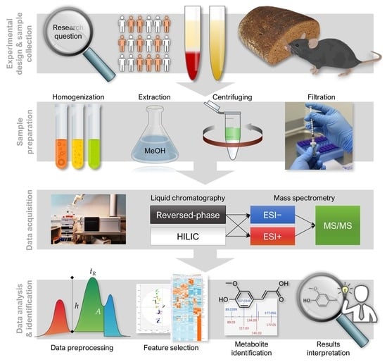
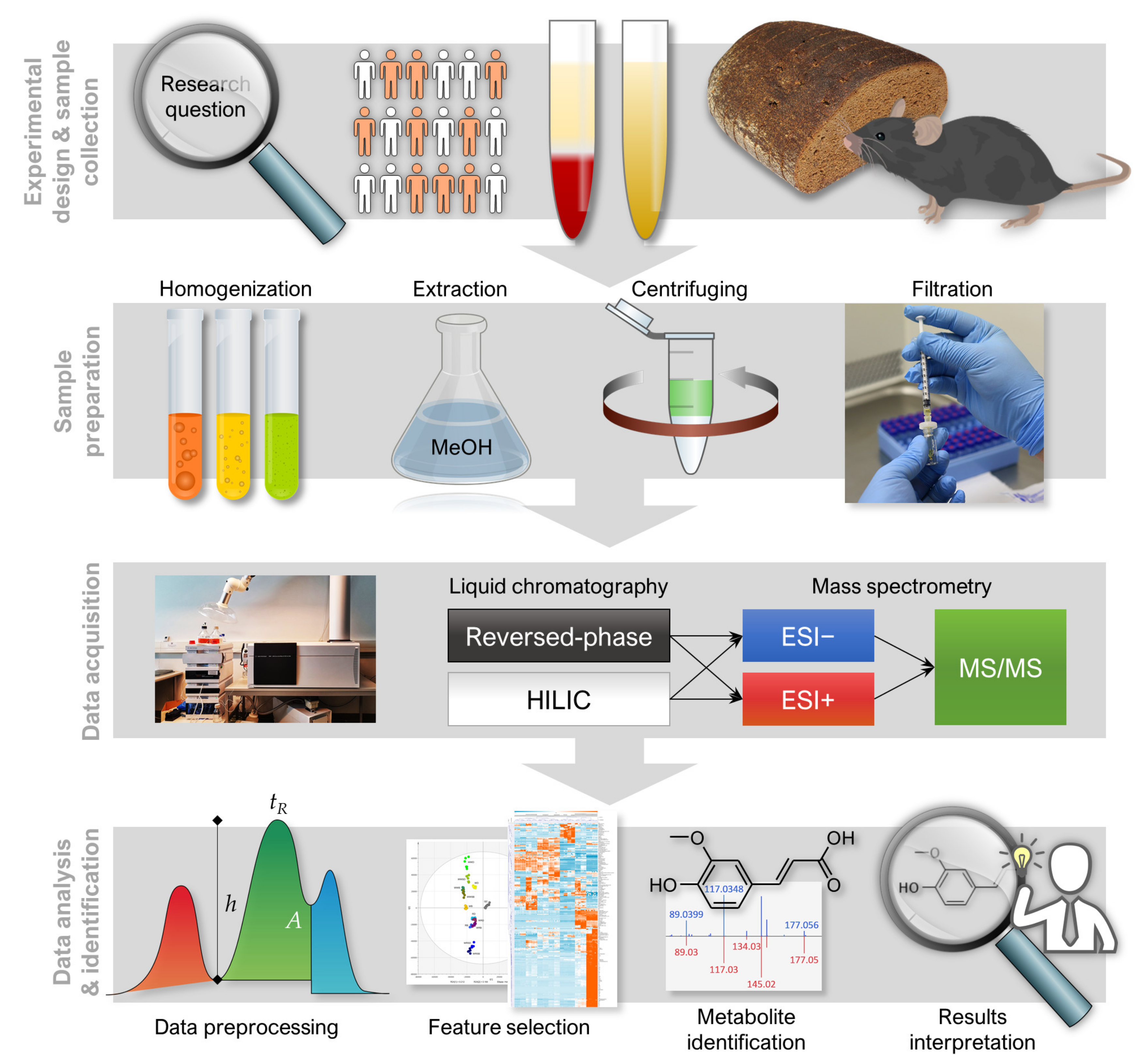
1. Introduction
2. Experimental Design
2.1. Materials
- a.
- 96-well plate (Thermo Scientific, Rochester, NY, USA, Cat.No. 260252),
- b.
- Filter plate (Agilent, Santa Clara, CA, USA, Cat.No. A5969002)
- c.
- 96-Well cap mats (Thermo Scientific, Roskilde, Denmark, Cat.No. 276002)
- d.
- Syringe filters (PALL Corporation, Ann Arbor, MI, USA, Cat.No. 4552T)
- e.
- Syringe Norm-Ject® tuberculin 1 mL (Henke Sass Wolf, Tuttlingen, Germany, Cat.No 4010-200V0)
- f.
- Wide orifice pipette tips (Thermo Scientific, Vantaa, Finland, Cat.No. 9405050)
- g.
- Homogenizer microtubes (OMNI International, Kennesaw, GA, USA, Cat.No 19-620
- h.
- Reversed-phase chromatography (RP) column: Zorbax Eclipse XDB-C18, particle size 1.8 µm, 2.1 × 100 mm (Agilent Technologies, Santa Clara, CA, USA, Cat.No. 981758-902).
- i.
- Hydrophilic interaction chromatography (HILIC) column: Acquity UPLC BEH Amide 1.7 µm, 2.1 × 100 mm (Waters Corporation, Milford, MA, USA, Cat.No. 186004801).
- a.
- Acetonitrile, ACN (HiPerSolv CHROMANORM, VWR Chemicals, Fontenay-sous-Bois, France, Cat.No. 83640.320)
- b.
- Methanol, MeOH (CHROMASOLV™ LC–MS Ultra, Riedel-de Haën™, Honeywell, Seelze, Germany, Cat.No. 14262-2L)
- c.
- Formic acid (Optima LC/MS, Fisher Chemical, Geel, Belgium, Cat.No. A117-50)
- d.
- Ammonium formate (CHROMASOLV™ LC–MS Ultra, Honeywell Fluka, Seelze, Germany, Cat.No. 14266-25G)
- e.
- Ultra-pure water (Class 1, ELGA PURELAB Ultra Analytical, Lane End, UK)
2.2. Equipment
- a.
- Centrifuges: For 96-well plates: Heraus Megafuge 40R (ThermoFisher Scientific, Osterode, Germany), for microcentrifuge tubes: Centrifuge 5804R (Eppendorf, Hamburg, Germany)
- b.
- Vortex: Vortex Genie 2 (Scientific Industries, Bohemia, NY, USA)
- c.
- Homogenizer: Bead Ruptor 24 Elite with OMNI BR CRYO unit (OMNI International, Kennesaw, GA, USA)
- d.
- Shaker: Multi Reax (Heidolph, Schwabach, Germany)
- e.
- 1290 Infinity Binary UPLC system (Agilent Technologies, Waldbronn, Karlsruhe, Germany)
- f.
- 6540 UHD accurate-mass quadrupole-time-of-flight mass spectrometer (qTOF-MS) with Jetstream ESI source (Agilent Technologies, Santa Clara, CA, USA)
- g.
- Agilent MassHunter Acquisition B.07.00 (Agilent Technologies),
- h.
- MS-DIAL version 3.70 [17],
- i.
- MS-FINDER version 3.24 [18],
- j.
- R version 3.5.0 [19]
- k.
- Multiple Experiment Viewer (MeV) version 4.9.0 (http://mev.tm4.org/).
3. Analytical Procedure and Results
3.1. LC–MS Analysis
3.1.1. Sample Preparation
- 1.
- Thaw plasma/serum samples in ice water and keep them on wet ice during all the waiting periods.
- 2.
- Place the 96-well plate on wet ice for sample preparation and set the filter plate on it.
- 3.
- Add 400 μL of cold ACN to the filter plate well.
- 4.
- Vortex a plasma/serum sample 10 s at the maximum speed.
- 5.
- Add 100 μL of plasma/serum sample to the same well as ACN.
- 6.
- To prepare the pooled quality control (QC) samples, collect 10 μL aliquots of each sample and add them to the same clean microcentrifuge tube and finally, mix properly.
- 7.
- Mix ACN and sample by pipetting four times. Use wide orifice Finn Pipette tips to avoid tip clogging.
- 8.
- Repeat steps 1–5 for all samples. Lastly, use the same procedure for the QC sample. For the extraction blank, perform step 3 (cold ACN without sample) and use the same procedure thereon.
- 9.
- Filter the precipitated samples by centrifuging the plate for 5 min at 700× g at 4 °C.
- 10.
- Remove the filter plate and seal the 96-well plate tightly with the 96-well cap mat to avoid sample evaporation.
- 11.
- Analyze the samples immediately or store the plate at +4 °C for a maximum of 1 day or at −20 °C until analysis.
- 12.
- Weigh a maximum of 300 mg frozen tissue into 2-mL OMNI microtube with beads. Keep the samples on dry ice.
- 13.
- Add ice cold 80% methanol in a ratio of 500 µL solvent per 100 mg tissue and keep the tubes on wet ice. Include an extraction blank with solvent only.
- 14.
- Optional step: In the case of metabolite-dense sample material (e.g., plants), it might be necessary to use a more diluted solvent/sample ratio to avoid analytical problems, such as saturation of the detector or overloading of the column.
- 15.
- Homogenize samples with a Bead Ruptor 24 Elite homogenizer. For soft tissues, perform one homogenization cycle at the speed 6 m/s at +/− 2 °C for 30 s.
- 16.
- Optional step: In case a homogenizer instrument is not available, manual tissue disruption can be performed using mortar and pestle with liquid nitrogen.
- 17.
- Extract the homogenized samples in a shaker for 5 min at RT.
- 18.
- Centrifuge samples for 10 min at 20,000× g at +4 °C.
- 19.
- Collect the supernatants on a 96-well filter plate and centrifuge for 5 min at 700× g at 4 °C.
- 20.
- Optional step: Filter the samples using solvent resistant syringes and PTFE filters into the HPLC vials.
- 21.
- Take aliquots (5–25 μL) of filtered samples and combine into one vial to be used as QC sample in the analysis.
- 22.
- Analyze the samples immediately or store the plate at +4 °C maximum of 1 day or −20 °C until analysis.
3.1.2. LC–MS Measurement
- 23.
- Use the following conditions for RP chromatography: Column oven temperature 50 °C, flow rate 0.4 mL/min, gradient elution with water (eluent A) and methanol (eluent B) both containing 0.1% (v/v) of formic acid. Gradient profile for RP separations: 0–10 min: 2 → 100% B; 10–14.5 min: 100% B; 14.5–14.51 min: 100 → 2% B; 14.51–16.5 min: 2% B. Needle wash with 50% ACN. Set the injection volume at 2 μL and sample tray at 10 °C.
- 24.
- Use the following conditions for HILIC: Column oven temperature 45 °C, flow rate 0.6 mL/min, gradient elution with 50% v/v ACN in water (eluent A) and 90% v/v ACN in water (eluent B), both containing 20 mM ammonium formate (pH 3). The gradient profile for HILIC separations: 0–2.5 min: 100% B, 2.5–10 min: 100% B → 0% B; 10–10.01 min: 0% B → 100% B; 10.01–12.5 min: 100% B. Needle wash with 50% ACN. Set the injection volume at 2 μL and sample tray at 10 °C.
- 25.
- To operate at high mass accuracy (<2 ppm), calibrate the MS daily and use the continuous mass axis calibration by monitoring two reference ions from an infusion solution throughout the analytical runs. Examples of reference ions in ESI+ mode: m/z 121.050873 and m/z 922.009798, and reference ions in ESI− mode m/z 112.985587 and m/z 966.000725. These reference ions are coming from the compounds in the infusion solution. m/z 121 is purine, m/z 112 is trifluoroacetic acid and m/z 922 and 966 are HP-0921 (Hexakis (1H,1H,3H-tetrafluoropropoxy) phosphazine) [20,21]
- 26.
- Use the following conditions for Jetstream ESI source: drying gas temperature 325 °C and flow 10 L/min, sheath gas temperature 350 °C with a flow of 11 L/min, nebulizer pressure 45 psi, capillary voltage 3500 V, nozzle voltage 1000 V, fragmentor voltage 100 V and skimmer 45 V. Use nitrogen as the instrument gas.
- 27.
- For data acquisition, use a 2 GHz extended dynamic range mode in both ESI + and ESI - ionization modes from m/z 50 to 1600 (may be adjusted according to sample matrix). Collect the data in the centroid mode at an acquisition rate of 1.67 spectra/s (i.e., 600 ms/spectrum) with an abundance threshold of 150. For automatic data dependent MS/MS analyses, set the precursor isolation width to 1.3 Da. From every precursor scan cycle, 4 most abundant ions are selected for fragmentation. These ions are excluded after two product ion spectra and released again for fragmentation after a 0.25 min hold. Product ion scan time is based on precursor ion intensity, ending at 25,000 counts or after 300 ms. Use collision-induced dissociation voltage 10, 20 and 40 V in subsequent runs.
- 28.
- Generate the worklist containing analytical samples. Inject quality control samples after every 12 samples and before and after the sample sequence. To monitor contamination during sample preparation and liquid chromatography, inject extraction blanks in the beginning (before the QC samples) and end of the analysis. The injection order of samples should be randomized. If the study contains samples from multiple matrices, such as samples from different organs, it is recommended that all the samples of a matrix be injected consecutively, for example first inject all heart samples, followed by all liver samples. If there are multiple samples from the same individual, it is recommended that the samples of an individual are run consecutively. We use an in-house developed software called Wranglr (github.com/antonvsdata/wranglr) to automate the generation of sample worklists by automatically randomizing the sample order and adding QC and MS/MS samples. Wranglr is an open-source web application developed with the Shiny package for R [22].
- 29.
- Inject 2 blanks and then 15–20 QC samples at the beginning of each run for column conditioning. Inject a QC sample after every 12 samples during the analysis. At the end of each run, include 4 QC samples: 1 for MS analysis, 3 for MS/MS analysis from 3 different collision energies and finally, 2 blanks. If the run contains samples from different tissues or species (i.e., different expected metabolite profiles), it is recommended to run the MS/MS analysis additionally from one sample per different sample type to increase the coverage of available MS/MS data.
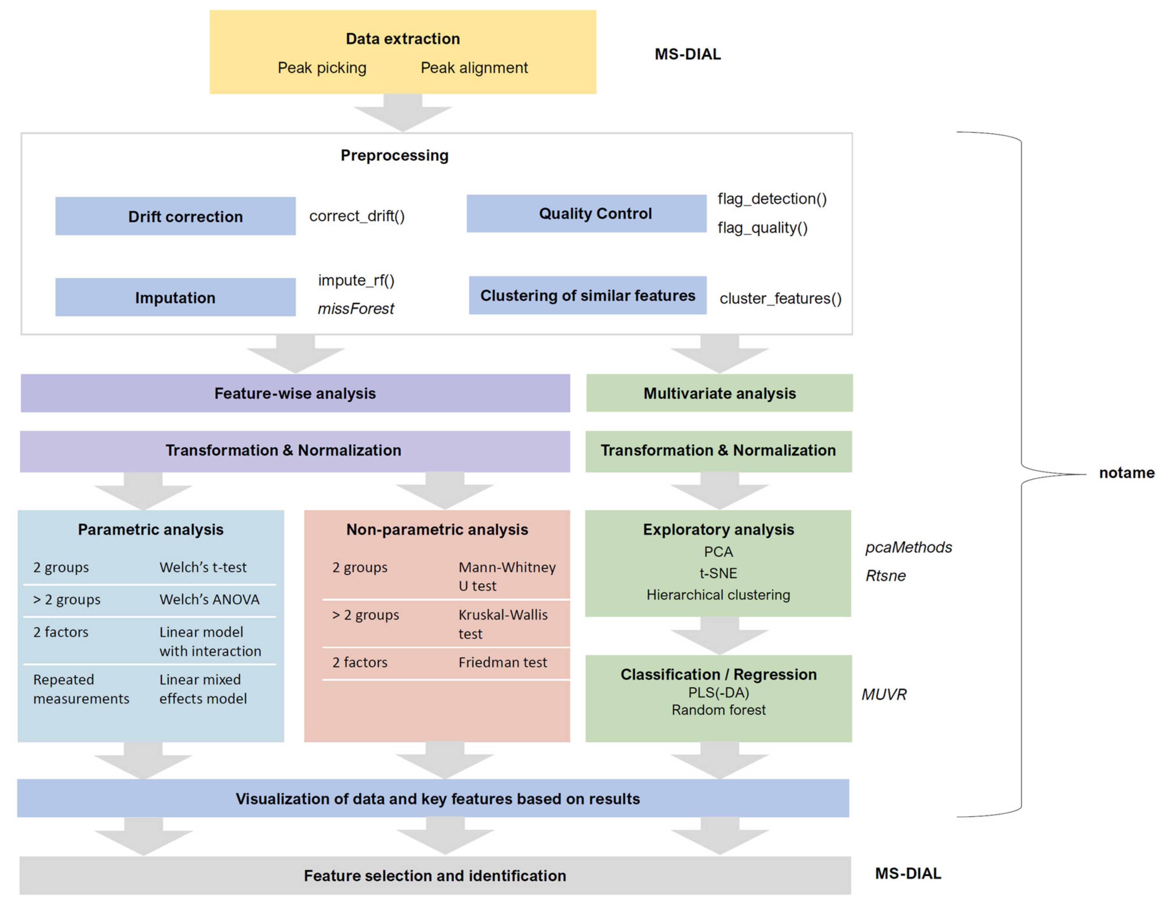
3.2. Data Collection and Preprocessing
3.2.1. Peak Picking and Alignment
- 30.
- Before the peak picking, convert the raw instrumental data (i.e., *.d) to ABF format using Reifycs Abf Converter (https://www.reifycs.com/AbfConverter). Follow the vendor-specific instructions on the website.
- 31.
- For the peak picking in MS-DIAL (version 3.70), choose the following parameters:
- a.
- m/z tolerance according to the instrument mass accuracy; however, it is advisable to set a bit higher tolerance to avoid screening out peaks close to the threshold, e.g., for QTOF we have used tolerance of 0.01 Da or 10 ppm.
- b.
- minimum peak height 2000 signal counts for QTOF (or at least 5 times the typical noise level of the instrument; 3000 signal counts for highly concentrated plant samples).
- c.
- mass slice width 0.1 Da (suitable for QTOF and other instruments with high mass accuracy).
- d.
- linear weighted moving average as the smoothing method (smoothing level 3 scans and minimum peak width 5 scans, according to developer recommendations).
- e.
- in positive mode, select [M + H]+, [M + NH4]+, [M + Na]+, [M + K]+, [M + CH3OH + H]+ and [M − NH3 + H]+ as the most typical adducts and in-source fragments; in negative mode, select [M − H]−, [M − H2O − H]−, [M + Cl]−, [M + HCOOH – H]− and [2M − H]− as the adducts and in-source fragments. Depending on previous knowledge, more adducts may be determined.
- 32.
- For the peak alignment, set the retention time tolerance according to method accuracy (for the present method we have used 0.05 min and MS1 tolerance at 0.015 Da. Set the detection filter (detected in at least one sample group) at 50%. Unselect the “detected in all QCs” option and select gap filling by compulsion.
- 33.
- Once the peak picking is finished, export the alignment result as peak areas into a raw data matrix as a tab-separated text file. Transform the data matrix into a datasheet in a spreadsheet software, such as Excel. Insert additional columns to each datasheet specifying the chromatography and the ionization mode before combining the datasheets into a single file. Remove columns containing peak areas from auto-MS/MS data files.
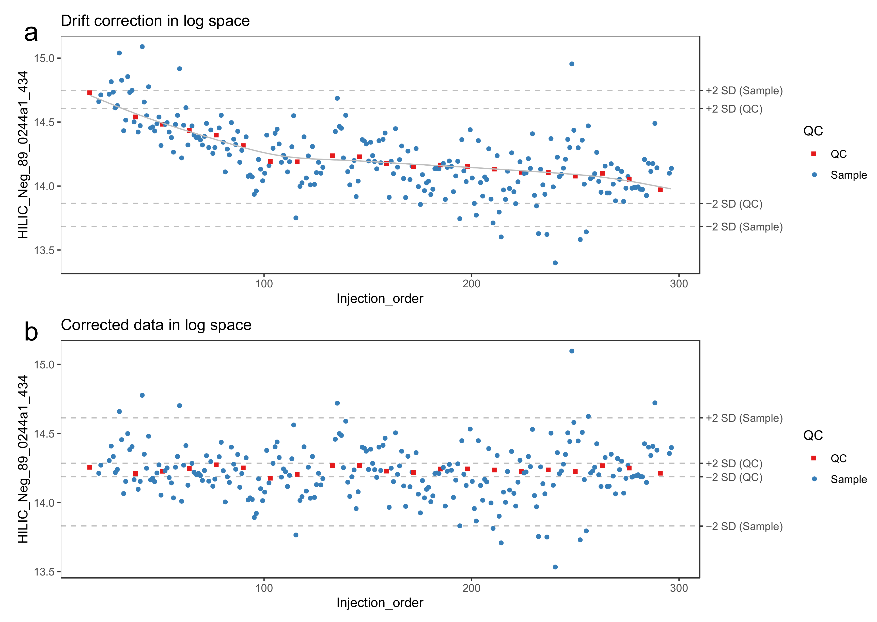
3.2.2. Drift Correction and Flagging Low-Quality Features
- 34.
- Make sure that missing values are correctly represented. A peak picking software might use a numerical value (such as 0, 1 or -999) to represent missing values, while other software such as R have specific ways of representing missing values. For more information on handling missing values, see Section 3.2.4.
- 35.
- Molecular features with too low detection rate in the QC samples should be flagged. We recommend a threshold is 70%, meaning that a molecular feature needs to be detected in at least 70% of the QC samples.
- 36.
- Log-transform the features prior to drift correction. Log-transformed data normally conform better with the assumptions of the regression model used to model the drift. We use the natural logarithm. Replace zeroes with a value slightly above one (e.g., 1.1) to make sure that all log-transformed values are > 0.
- 37.
- The drift correction should then be performed by repeating steps 38–40 for each molecular feature. These procedures are included in notame (function correct_drift()).
- 38.
- Model the drift function (fdrift) by fitting a smoothed cubic spline [23] to the QC samples, where the abundance of the molecular feature is predicted by the injection order Figure 3a. Smoothed cubic spline regression has one hyperparameter: a smoothing parameter, which controls the overall curvature of the drift function. The smoothing prevents the spline from overfitting the drift function in the presence of a few deviating QC samples (see Figure 4). A suitable value for the smoothing parameter is chosen by leave-one-out cross validation. For the R function smooth.spline, [24] we recommend the smoothing parameter to be between 0.5 and 1.5.
- 39.
- Correct the abundance of each sample using the following formula (for a sample with injection order i):
- 40.
- Reverse the log transformation by applying the corresponding exponential function.
- 41.
- The drift correction procedure is visualized (Figure 3 and Figure 4) by drawing a scatter plot of the abundances against the injection order before and after drift correction. A line representing the drift function should be added to the scatter plot before correction. To reduce the amount of manual inspection, we usually only inspect potential candidate molecular features selected from downstream statistical tests.
- 42.
- Optional step: Compute the quality metrics after drift correction and keep only the drift-corrected values for the molecular features where the change in quality metrics indicate that the data quality has been improved. For the other molecular features, retain the original values.
- 43.
- Flag or remove low-quality features. As recommended by Broadhurst et al. [10], only the molecular features with RSD < 0.2 and D-ratio < 0.4 should be retained. In notame, this can be done with the function flag_quality().
3.2.3. Quality Control
- 44.
- Draw the visualizations in steps 46-52 before drift and after drift correction.
- 45.
- Flag low-quality features to monitor data quality and the effect of preprocessing.
- 46.
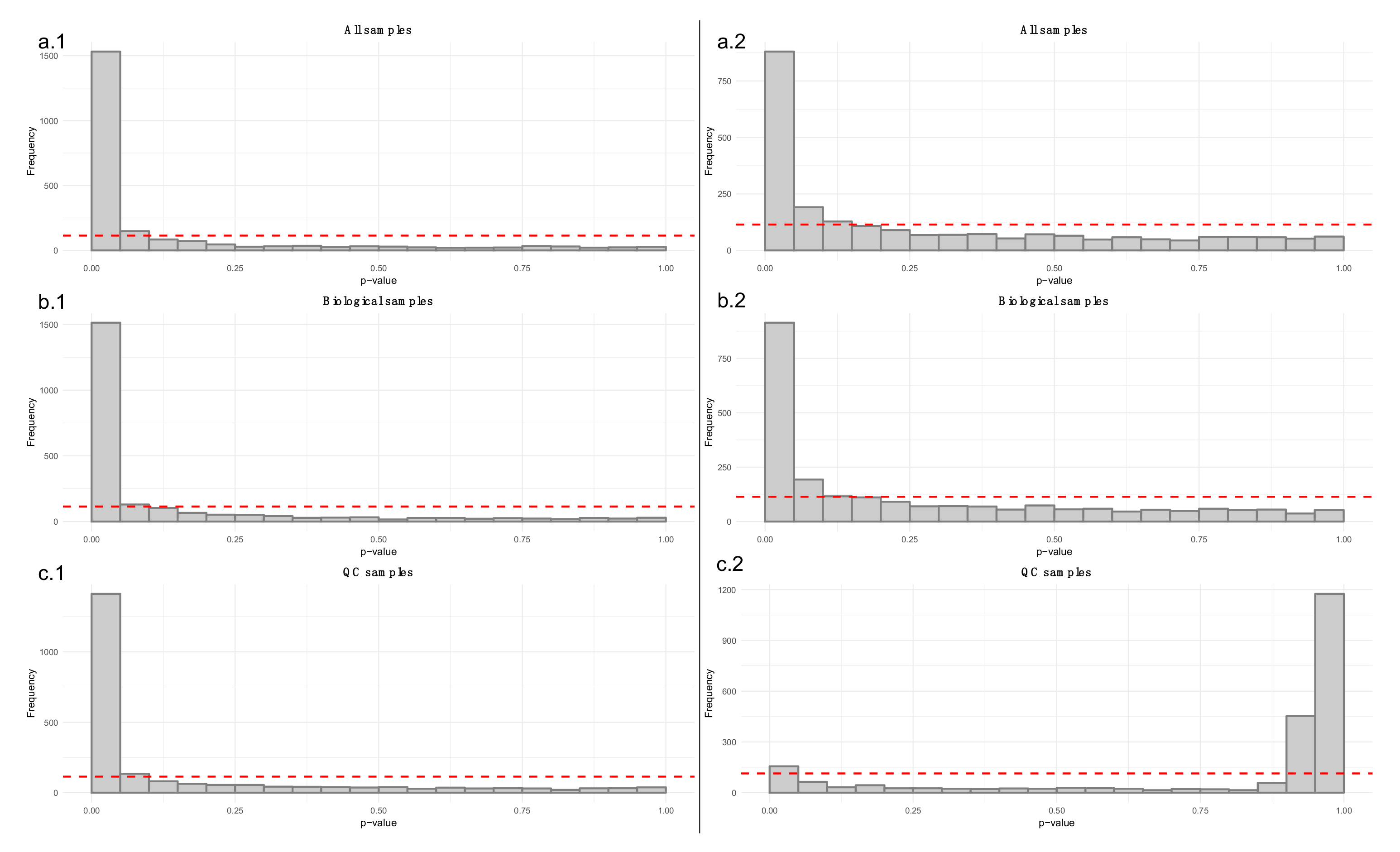
- Apply a linear model to each feature, where the feature levels are predicted by injection order. Fit the model separately for QC samples, biological samples and all samples. Then visualize the effect of drift correction to individual features by drawing histograms of the p-values for the regression coefficient of injection order (Figure 5). We represent the expected uniform distribution by a horizontal line. Ideally, the p-values should roughly follow the expected uniform distribution, which would mean that there is no systematic dependency between feature abundances and injection order [26]. Unfortunately, this is rarely the case, but the closer the distribution is to uniform, the better. It is recommended to apply this procedure separately on QC samples and biological samples, which allows observing the drift patterns in both parts of the dataset.
- 47.
- Draw boxplots (Figure 6) where each individual boxplot represents the distribution of all feature levels in a sample: in the first boxplot order the samples by study group (a.1, a.2) (and possibly time point). This can reveal systematic changes in the global feature levels across samples. In the second type (b.1, b.2) order the samples by injection order, highlighting the QC samples. This allows us to observe any systematic drift across the feature levels in the samples.
- 48.
- Before subsequent visualizations, mean center the features and divide by standard deviation.
- 49.
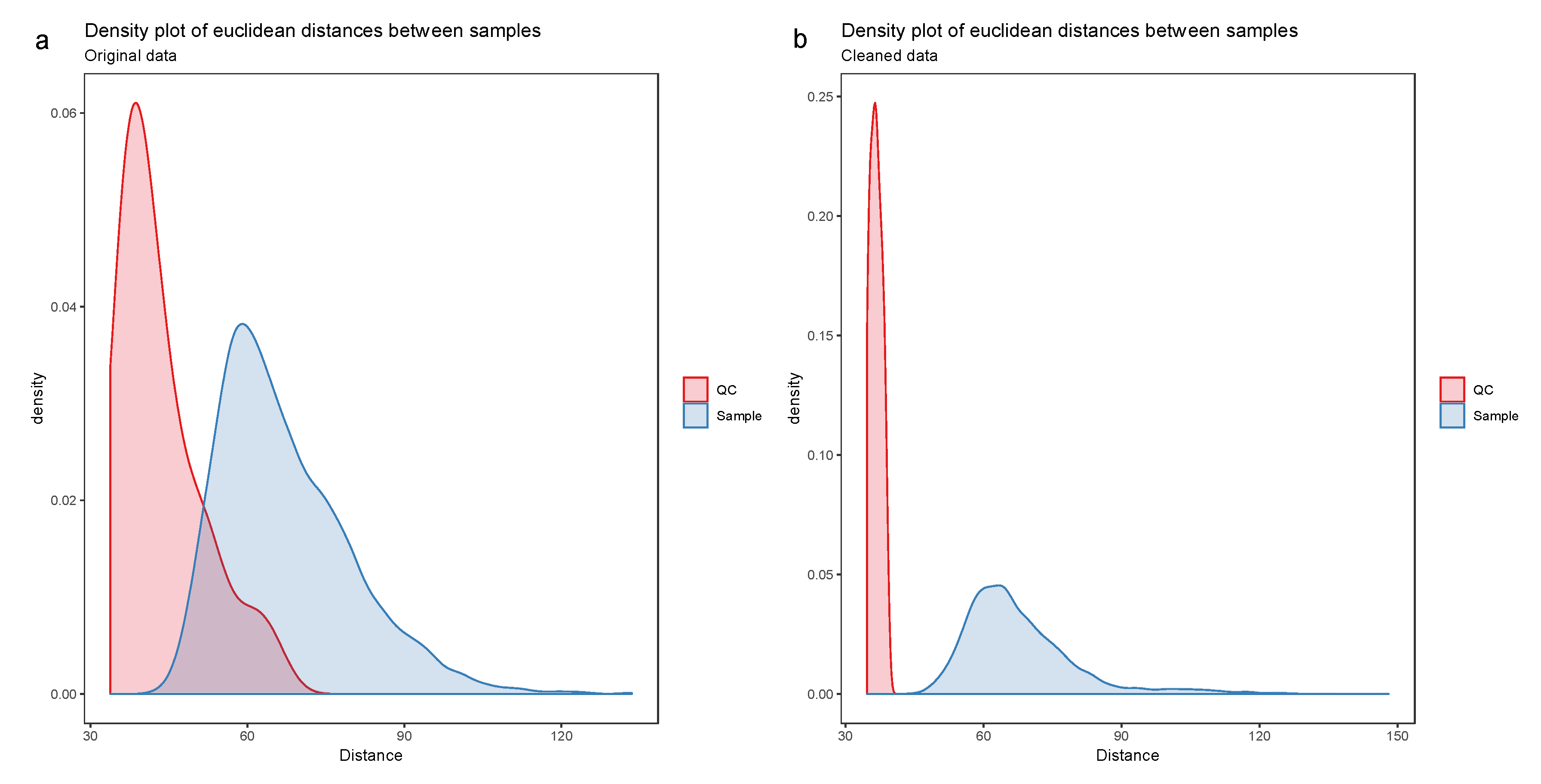
- Visualize the distribution of the Euclidean distances between samples using a density plot. The plot should feature two distributions, the distribution of distances between QC samples and the distances between biological samples. Ideally, the distribution of QC sample distances should be narrow and well separated from the distribution of study samples (Figure 7).
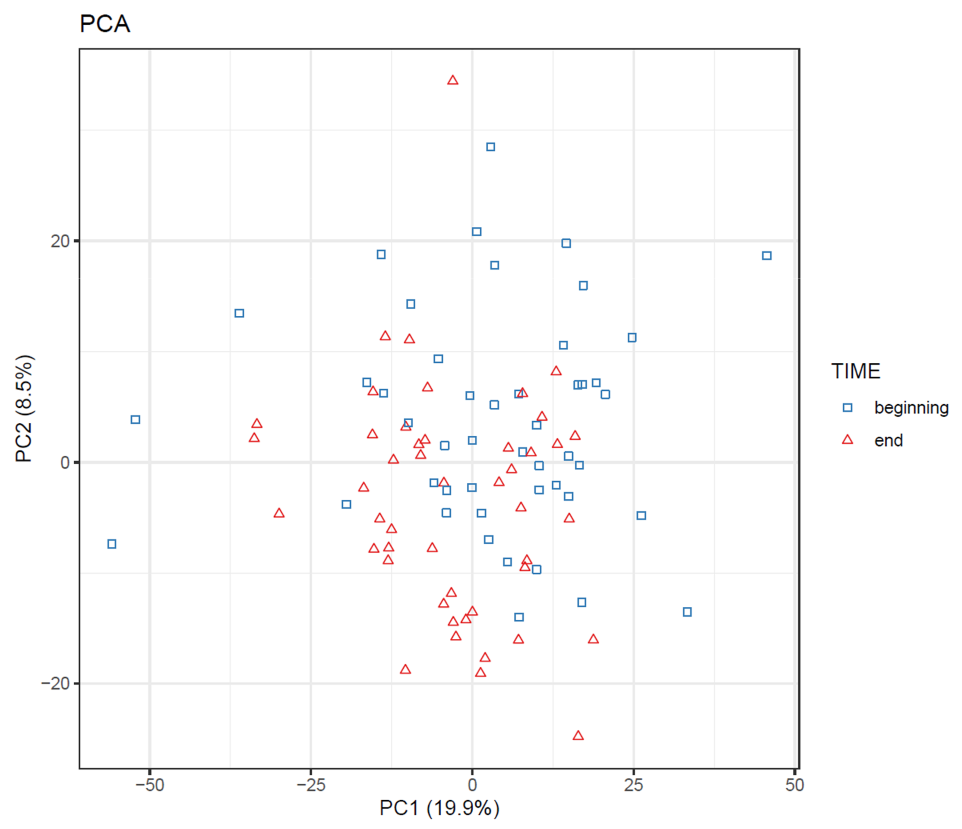
- 50.
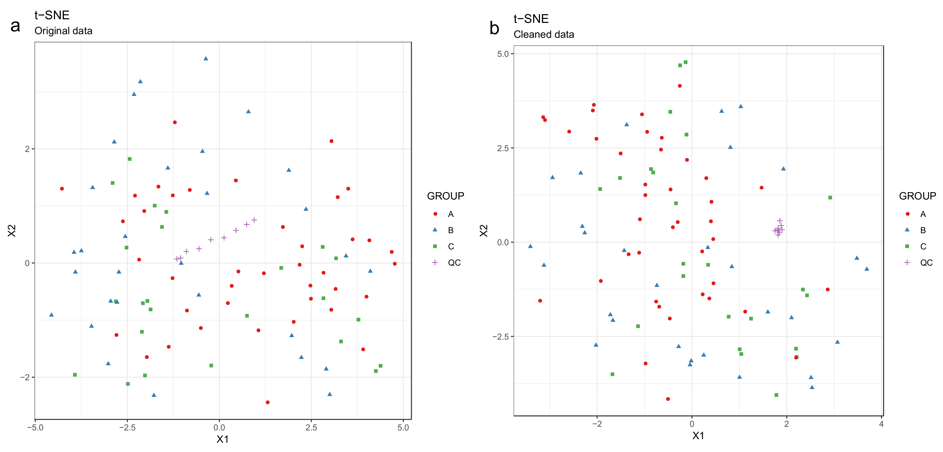
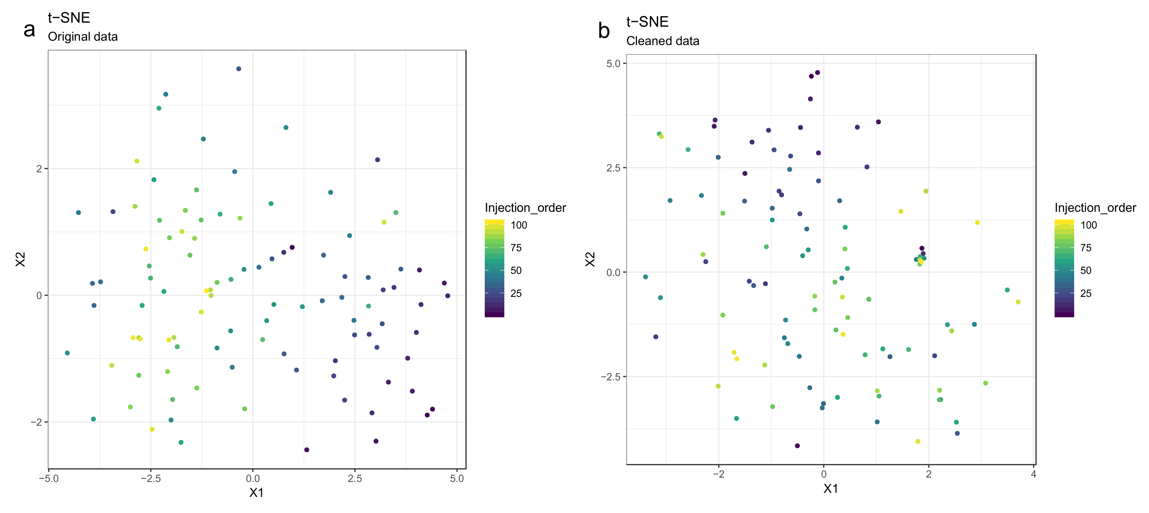
- Draw scatterplots of the data points using PCA and t-SNE. Samples can be highlighted by coloring the points in the scatter plot with a study factor (e.g., treatment groups or time points) to observe trends in the data. Ideally, QC samples should cluster together (Figure 8). We also draw separate plots where the samples are colored by injection order to observe drift patterns (Figure 9). If the data quality is high, there should be no visible patterns according to injection order (Figure 9b).
- 51.
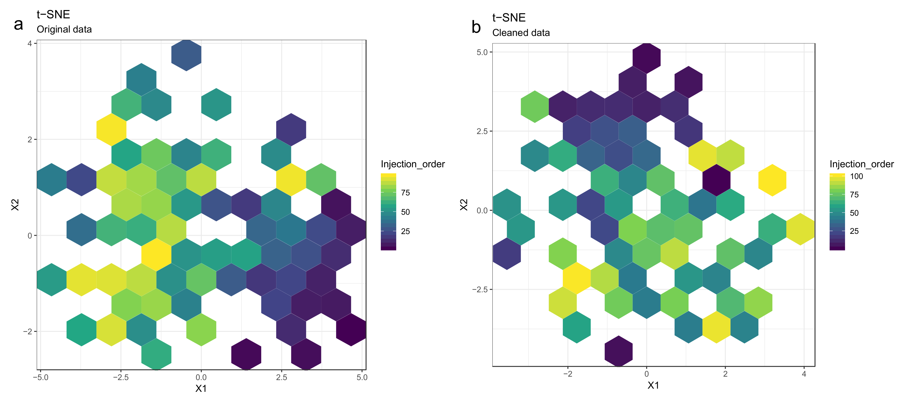
- Optional step: If there is a large number of samples and the points in the t-SNE plots tend to overlap, draw a hexbin version of t-SNE scatter plots colored by injection order (Figure 10), where the plot area is divided into hexagons and each hexagon is colored by the mean of the injection orders of the points inside that hexagon. As before, in an ideal case, there should be no visible drift patterns.
- 52.
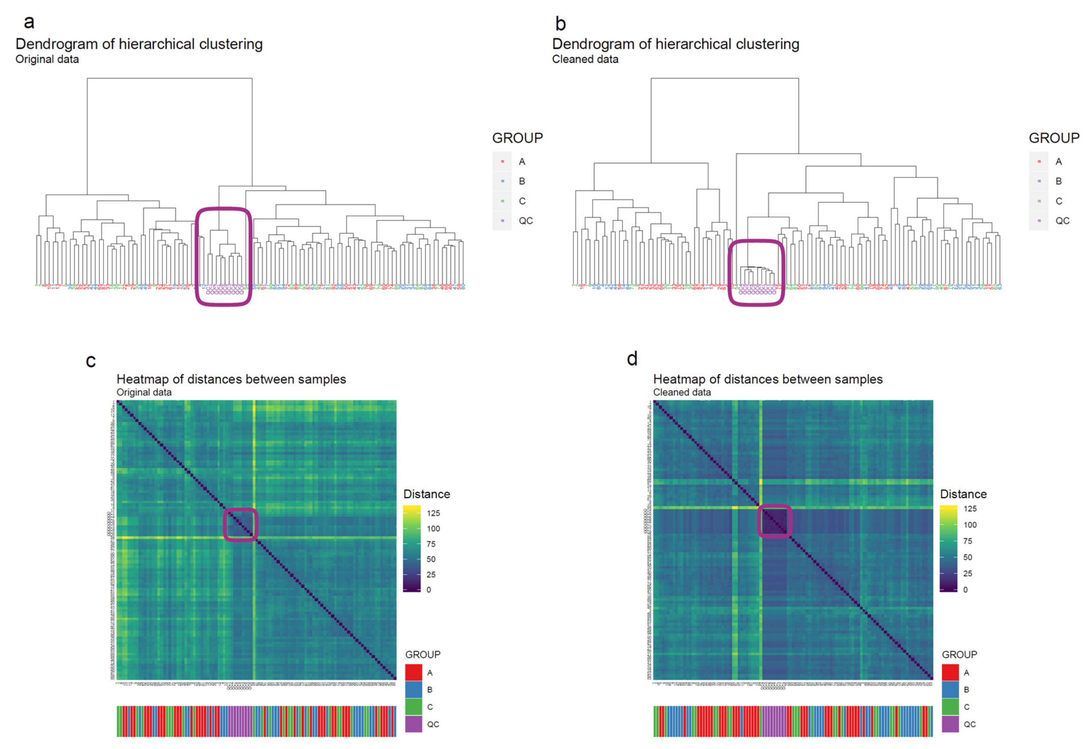
- Apply hierarchical clustering [31,32] to the samples and visualize the result in a dendrogram (Figure 11a,b). The QC samples should cluster together early. We also draw a heatmap (Figure 11c,d) representing pairwise distances between samples, where samples on the x and y axes are ordered by hierarchical clustering. The QC samples should have smaller inter-sample distances than other samples. Several techniques can be used for clustering. However, we have consistently achieved good results with hierarchical clustering using Euclidean distances and Ward’s criterion for linking clusters [32].
3.2.4. Imputation, Transformation, Normalization and Scaling
- 53.
- Impute missing values using random forest imputation. QC samples should be removed prior to imputation to ensure that the imputation is based on patterns in the biological data.
- 54.
- Transform the data using either natural logarithmic (nlog) or the generalized logarithmic (glog) function when the data are heavily skewed [38].
- 55.
- 56.
- Perform mean centering and scaling by standard deviation (autoscaling), before multivariate analysis; this is necessary with GLM-based methods as well as PCA and PLS-DA. However, this is not required for scale invariant techniques such as RF [40].
3.2.5. Clustering Molecular Features Originating from Same Metabolite
- 57.
- Cluster the molecular features from each analytical mode separately using the algorithm described above. Represent each cluster with the feature with the highest median abundance. Use these features for multivariate analysis and the clustering information for metabolite identification. The algorithm is provided in notame through the cluster_features() function.
3.3. Data Analysis
- 58.
- Combine the features from the different analytical modes to a single data matrix. In notame, this is achieved with the function merge_metabosets, which simply concatenates the data matrices and feature information tables row-wise (each row corresponds to a feature) and preserves the sample information unchanged. Note that combining analytical modes inevitably results in increased redundancy in the data matrix, as many compounds are detected in multiple analytical modes. However, combining the analytical modes is necessary so that all available information is available for multivariate analysis methods.
3.3.1. Feature-Wise (Univariate) Analysis
- 59.
- For study designs with two groups and no covariates, such as case versus control studies, use a simple Welch’s t-test, i.e., the extension of Student’s t-test to manage unequal variances between groups. For a non-parametric alternative, consider a Mann-Whitney U test.
- 60.
- For studies with multiple groups, first apply Welch’s one-way analysis of variance (ANOVA), which can manage unequal variances between groups, to select interesting features based on overall p-value. To investigate differences between groups, conduct post-hoc pairwise Welch’s t-tests.
- 61.
- For studies with two categorical study factors, apply two-way ANOVA, which allows examining the main effect of each factor and their interaction. If one or both factors have multiple levels, select interesting features based on overall p-values and conduct post-hoc pairwise t-tests as above (bullet 59). For a non-parametric alternative, consider Friedman test.
- 62.
- For studies with repeated measurements, use a linear mixed effects model with the time point, group and their interaction factors as fixed effects and the subjects as a random effect. If there are no more than two groups or time points, use t-tests on the regression coefficients to assess the significance of the effects. In the case of multiple groups and/or time points, use type III F-tests for ANOVA-like tables, e.g., with the help of the R packages lme4 and lmerTest that provide all the necessary tests [46,47].
- 63.
- To test the strength of association between molecular features or between molecular features and other variables, use Pearson correlation or Spearman correlation as a non-parametric alternative. This can also be done post-hoc, after identification of key metabolites [14].
- 64.
3.3.2. Multivariate Analysis
- 65.
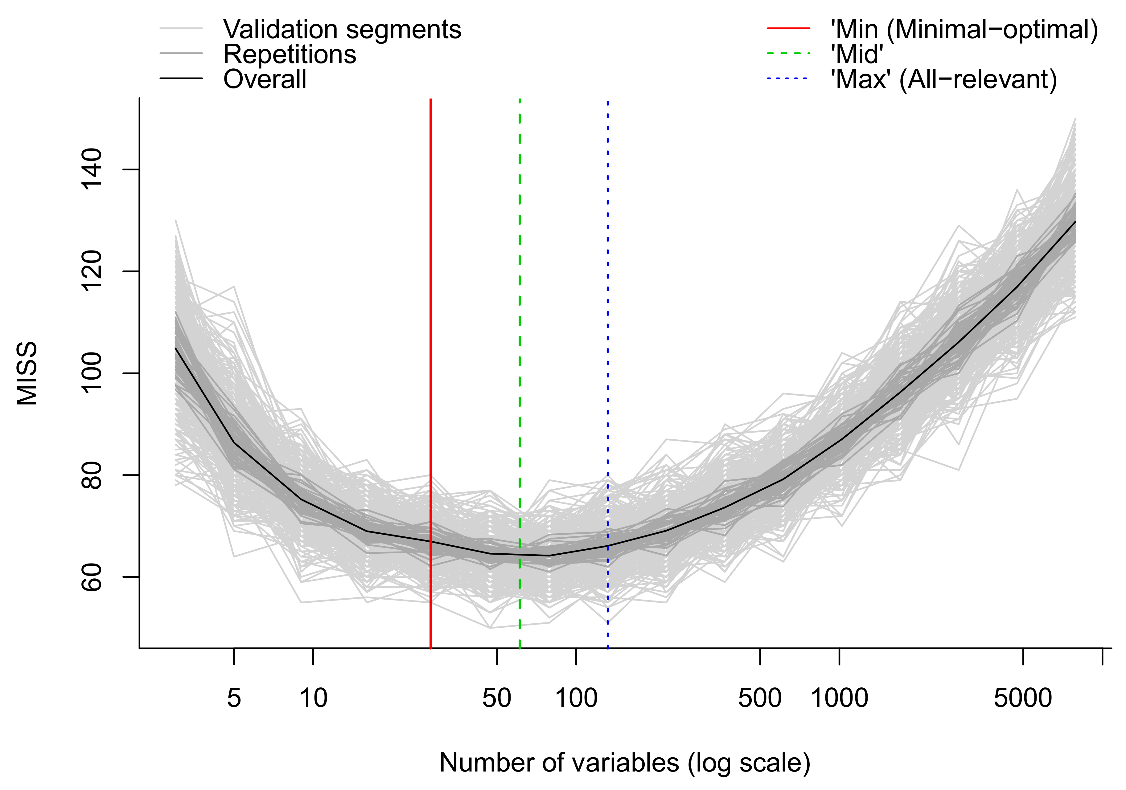
- Apply multivariate algorithms for prediction and variable selection. We employ the MUVR package in R which includes both RF and PLS [50]. For each analysis, three different models are obtained: the minimal-optimal (‘min’), ‘mid’ and all-relevant (‘max’) models (Figure 13). The ‘max’ model corresponds to maximum information content once the non-informative features have been removed and includes the highest numbers of relevant molecular features, thought it may include some redundant features or highly correlated features. This model is normally selected when e.g., pathway analysis will be applied afterwards. The ‘min’ model corresponds to the minimal-optimal set of molecular features where the strongest biomarker candidates are likely to be found. The ‘mid’ model corresponds to a compromise (geometric mean) between the ‘min’ and ‘max’ options, representing and with some redundancy between molecular features. In the end, the selection of the model depends on the research interest and study question, such as pathway analysis (‘max’), best prediction (‘mid’) or biomarker discovery (‘min’).
- 66.
- Optional Step: Follow this step if the MUVR package is not available (for example if other software than R is used). Evaluate performance of the multivariate model. Use cross-validation for PLS and out-of-bag error estimate for RF (for more information see [51])If the model performance is satisfactory, record variable importance metric (VIP value for PLS and rise in error rate for RF) for each feature.
3.3.3. Ranking and Filtering for Variable Selection
- 67.
- The first step is to sort the molecular features according to their ranks that received though the variable selection process, with the lowest rank or the most important rank (depending on the software) being the 1st rank and the biggest rank or the least important rank being the nth rank (n here is equal to the total number of molecular features available from the variable selection method). In the MUVR package, the output from the ‘min’, ’mid’ or’ max’ models provides the ranks for each of the molecular features already sorted by the smallest rank. The smallest rank represents that this particular molecular feature is the most important one.
- 68.
- Similarly, for each univariate model, the molecular features are sorted based on their q. The 1st rank is given for the feature with the lowest q-values from the FDR correction and the nth rank for the largest one.
- 69.
- Then, the rank from the RF model e.g., ‘mid’ model for each molecular feature is added together with the rank from the same molecular feature for the feature-wise model creating a new column with the Final Ranks.
- 70.
- The choice of the total number of the molecular features that are selected in the end for further analysis e.g., identification or pathway analysis is dependent strictly on the user.
- 71.
- Optional Step: In case the MUVR package is not used for variable selection, the procedure of ranking the molecular features stays the same for any type variable selection is chosen.
3.4. Visualization of Results
3.4.1. Feature-Wise Graphs
- 72.
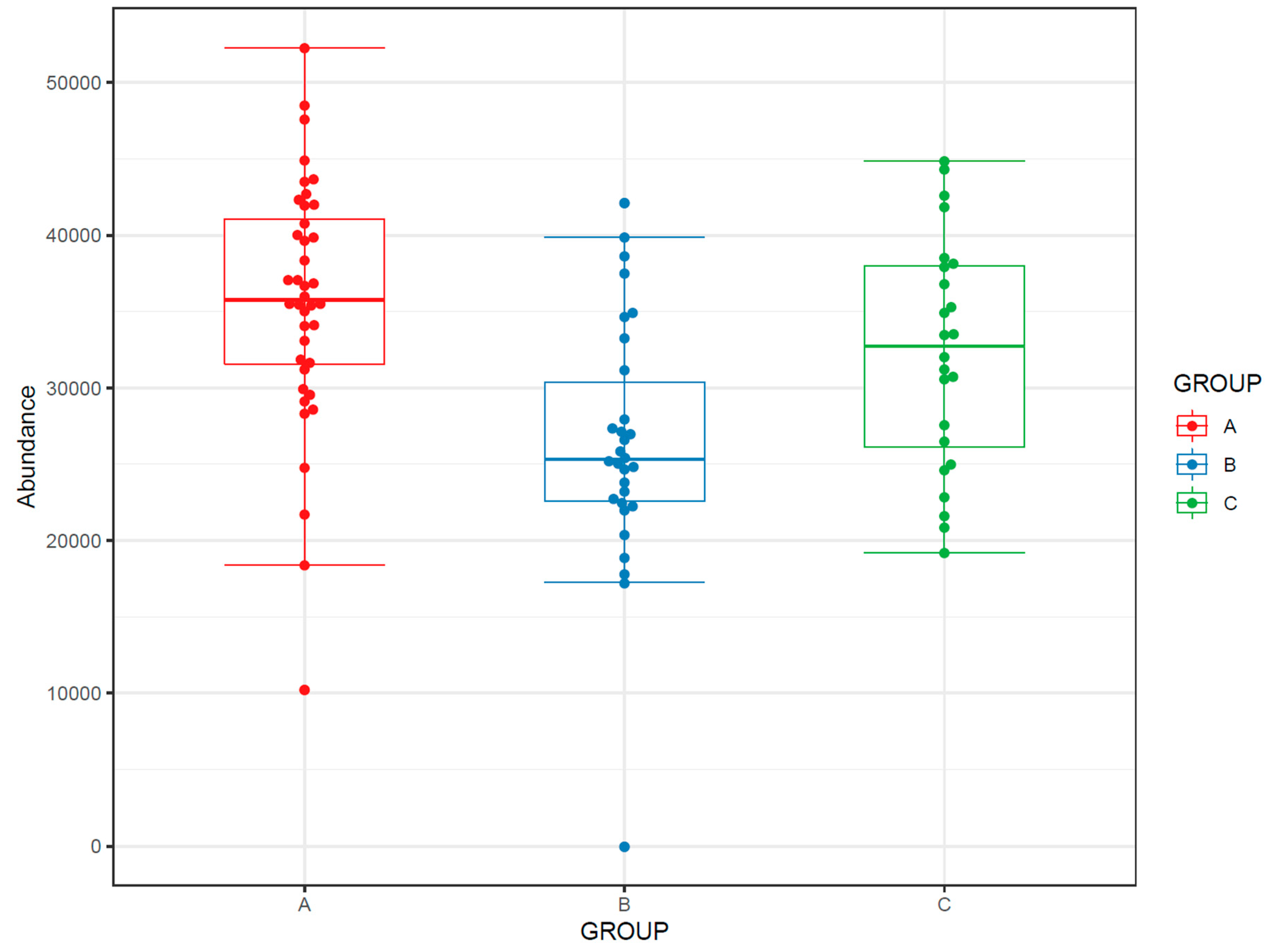
- If the study has multiple study groups, the differences between groups can be illustrated by beeswarm boxplots separately for each group (Figure 14).
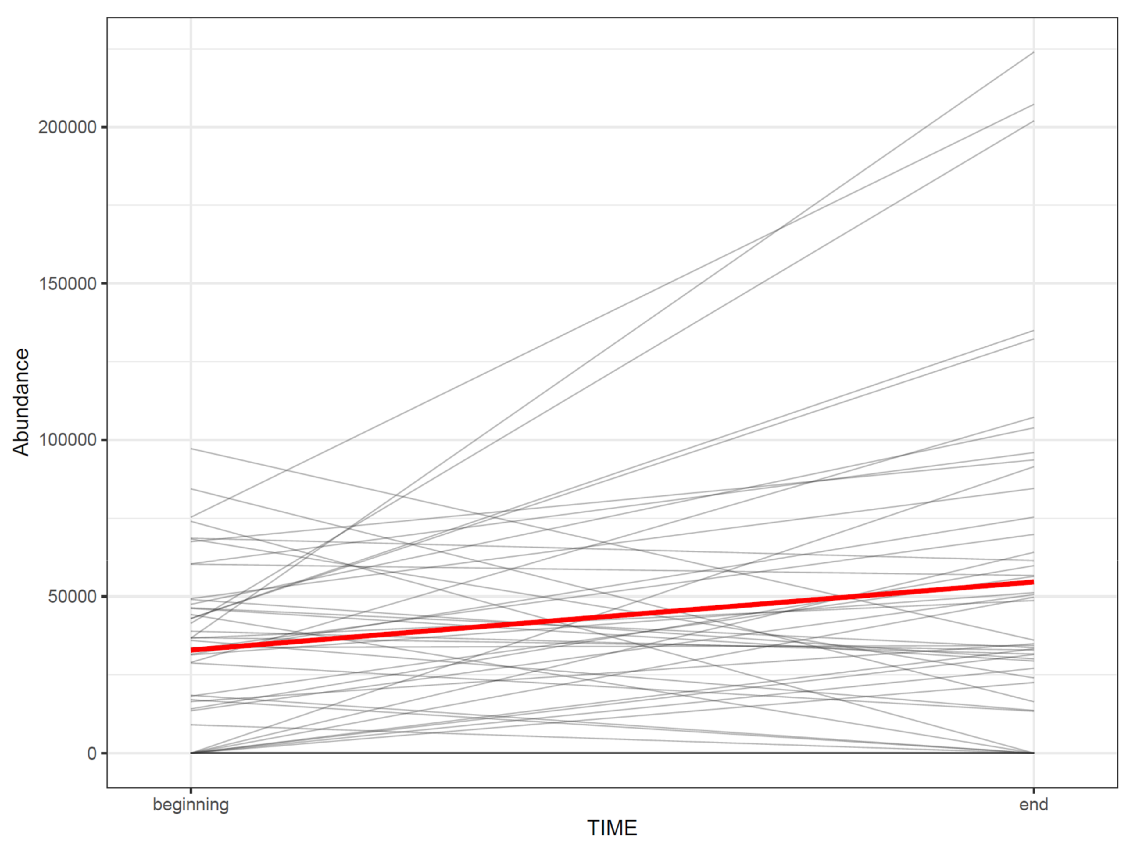
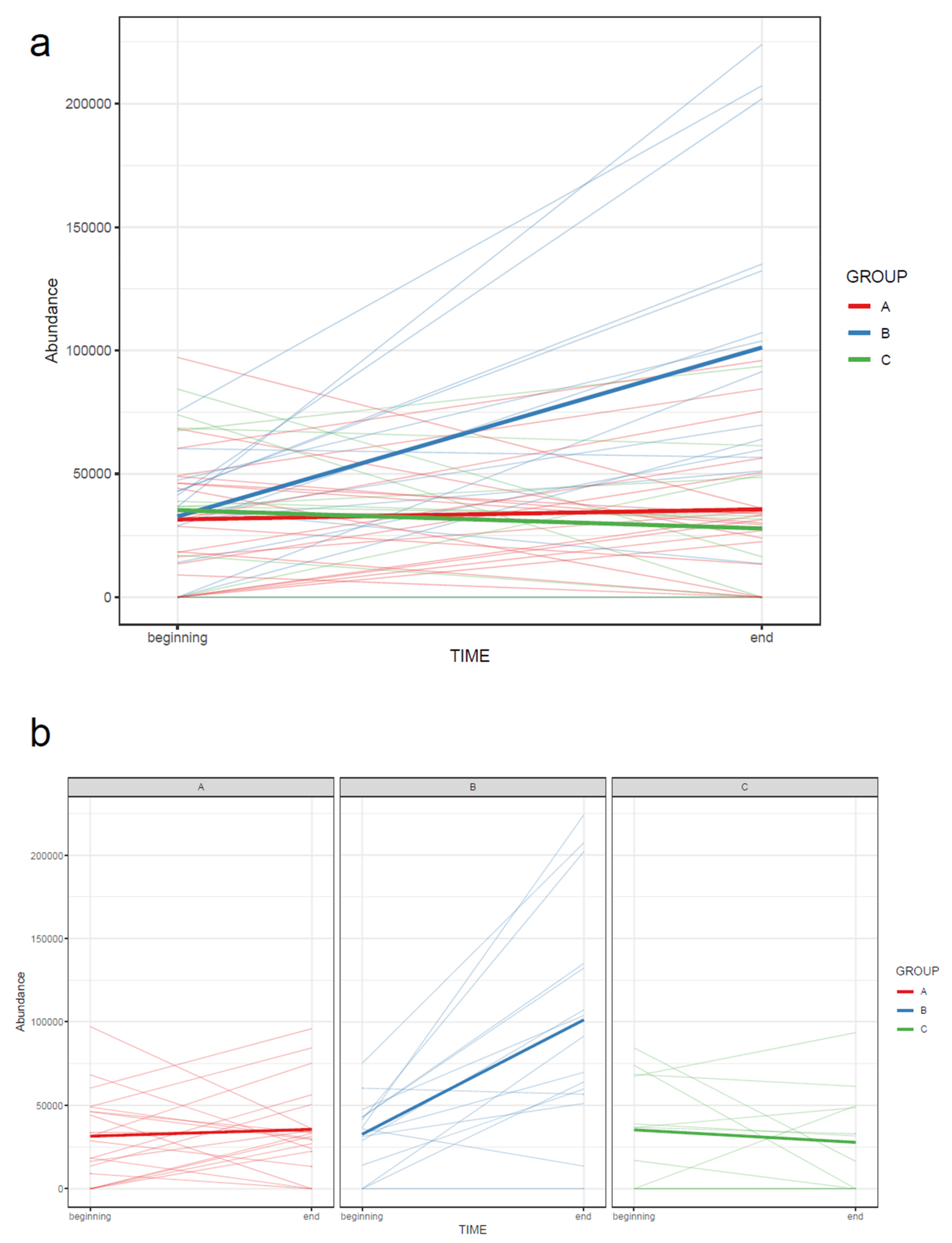
- 73.
- If the study contains samples from multiple time points, the effect of time can be visualized with a line plot using one line per subject together with a thicker line representing the mean at every time point (Figure 15).
- 74.
3.4.2. Comprehensive Visualization of Results
- 75.
- 76.
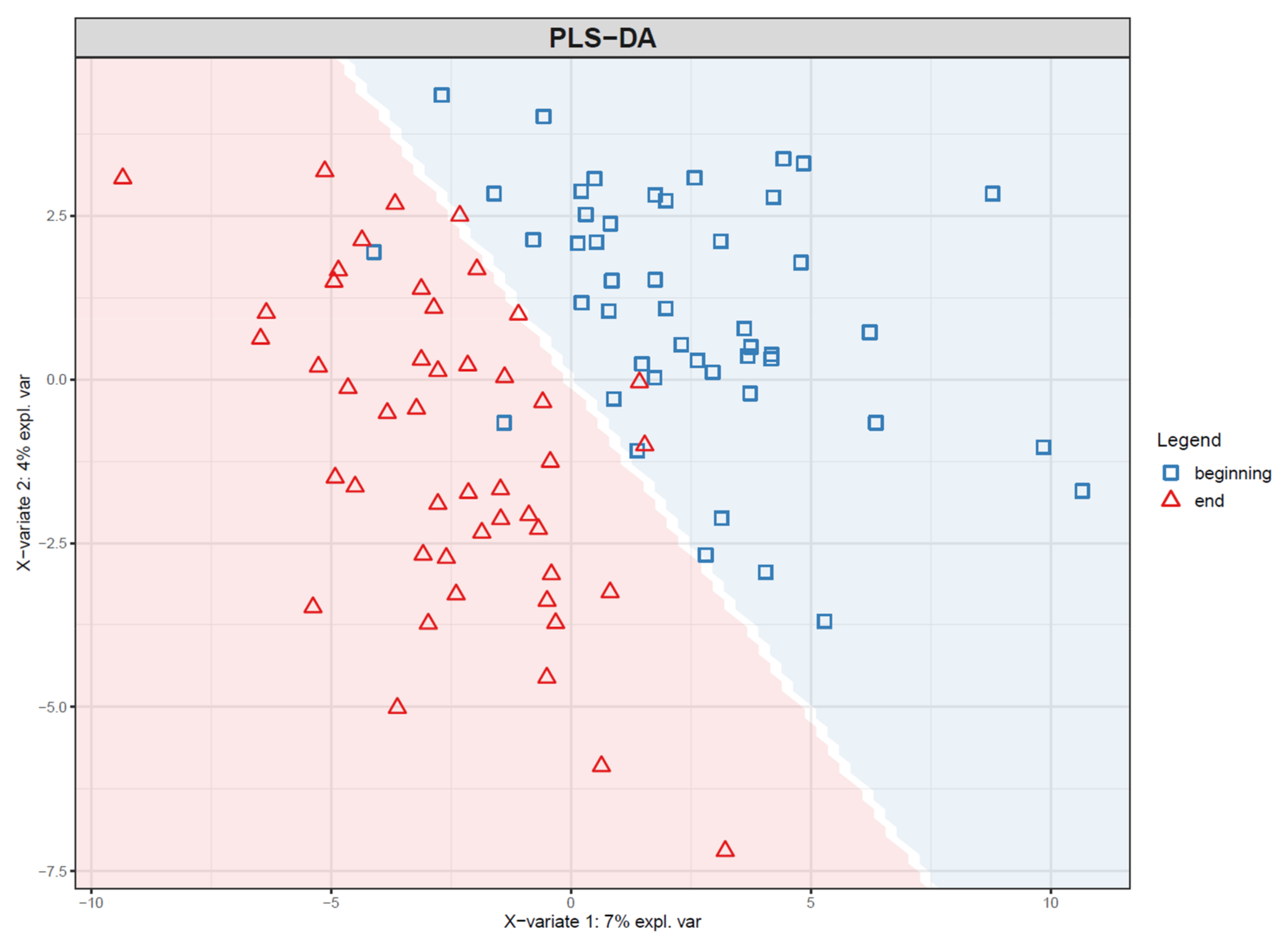
- If PLS(-DA) is used, visualize the samples in a PLS score plot (see Figure 19).
- 77.
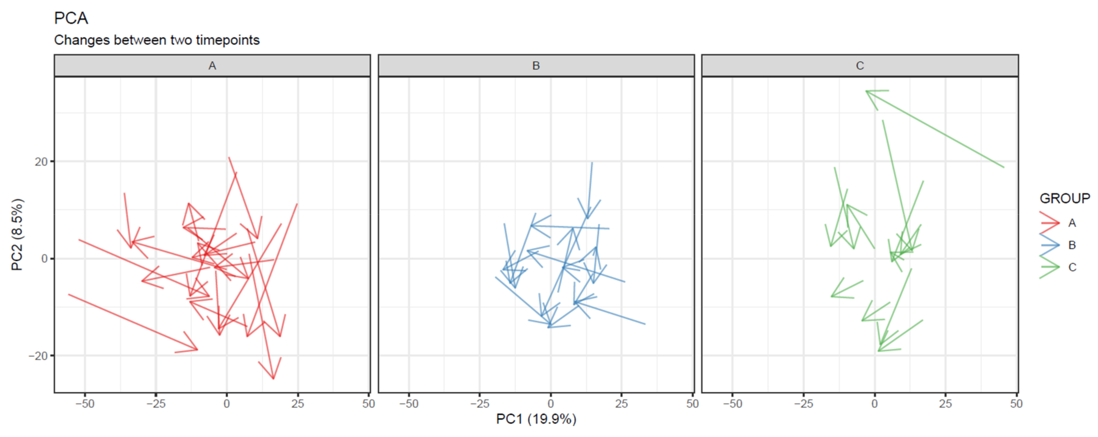
- To visualize overall changes with respect to time in studies with multiple time points, use PCA and t-SNE figures with arrows depicting change in each individual. The arrows should start at the first time point and end at the last time point for each individual. We recommend plotting each study group separately, as the plot can get crowded since the arrows occupy significantly more space than points (Figure 20).
- 78.
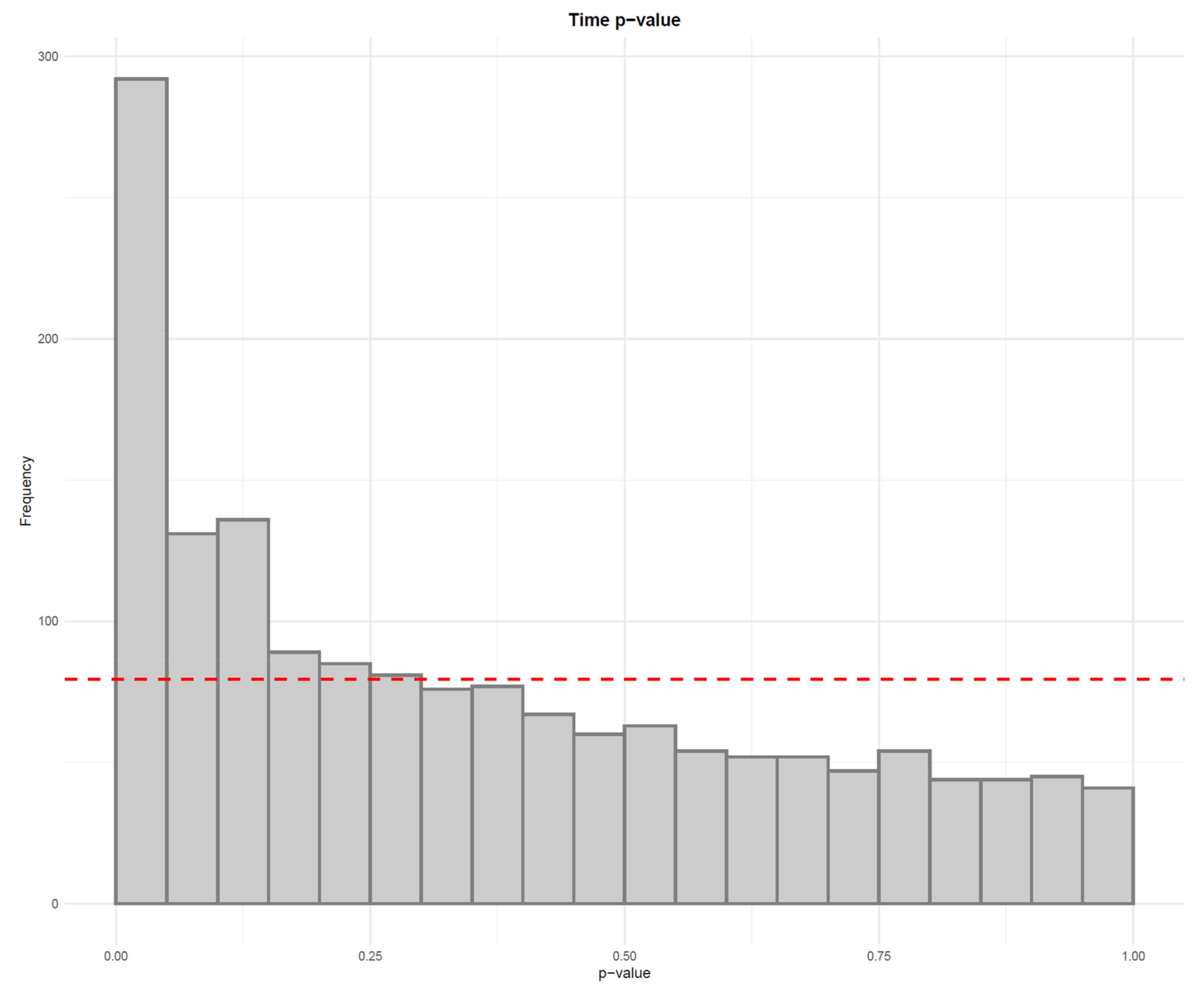
- Visualize the distribution of p-values from feature-wise analysis in a histogram. Use a line to depict the expected uniform distribution (under null hypothesis). If the distribution of the p-values deviates from the line as in Figure 21, it can be argued that we are observing a real effect.
- 79.
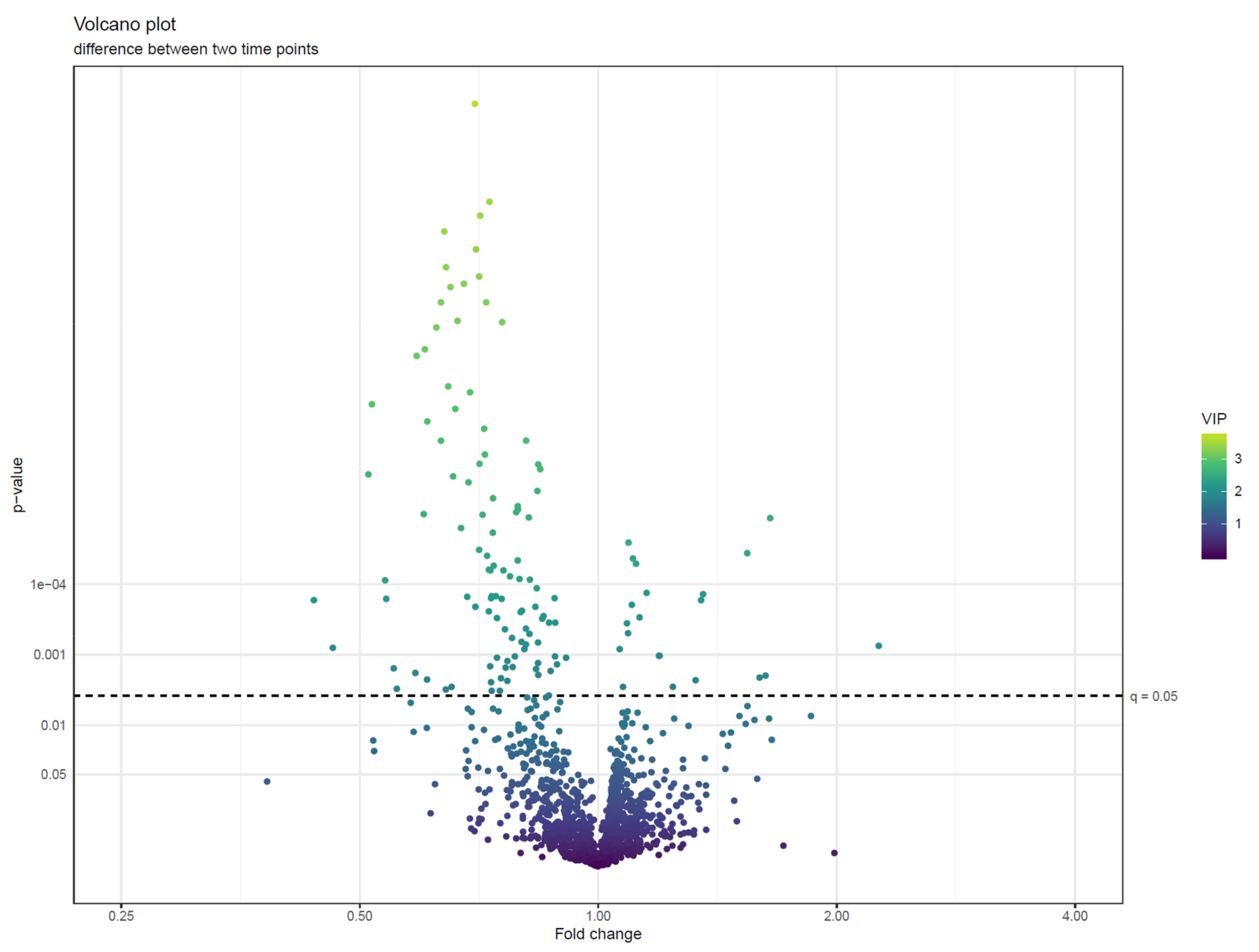
- Visualize the results of feature-wise tests in a volcano plot. Volcano plots are scatter plots with p-values on the y axis and effect size (such as fold change) on the x-axis. Add a horizontal line representing the significance threshold for FDR-adjusted q-values. To co-visualize multivariate results, the features can be colored by their relevance score in the multivariate prediction (Figure 22).
- 80.
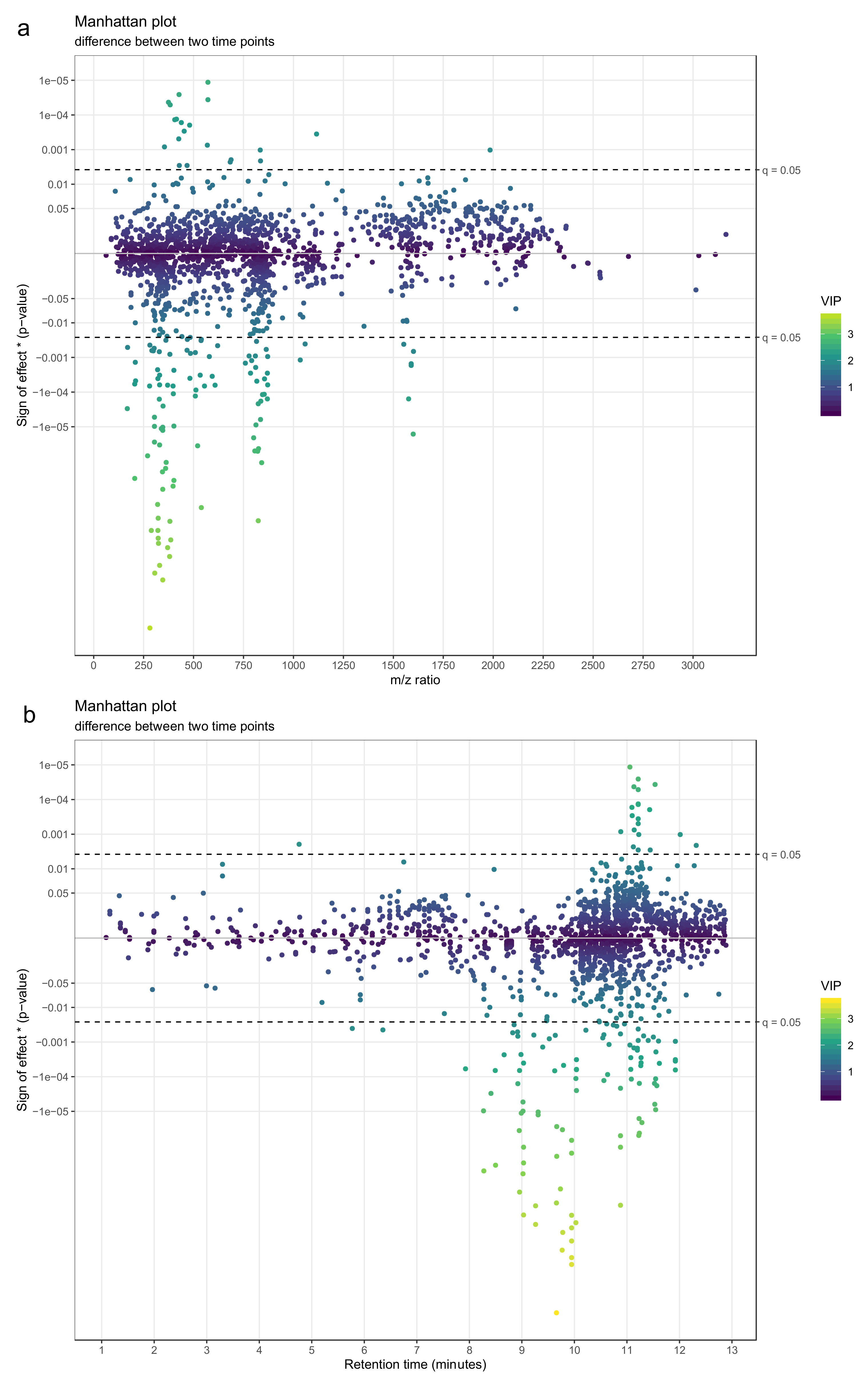
- Use a Manhattan plot to connect the results of statistics to biochemical properties of the molecular features. The Manhattan plot should have either retention time or mass-to-charge ratio as the x-axis and –log10(p-value) on the y-axis. For a directed Manhattan plot, multiply –log10(p-value) by the sign of the effect. The points in the Manhattan plot can be colored by the respective VIP value from PLS-DA or another similar metric. Similar to volcano plots, add a horizontal line to represent the significance threshold for FDR-adjusted q-values. Figure 23a,b show Manhattan plots with mass-to-charge ratio and retention time on the x-axis, respectively.
- 81.
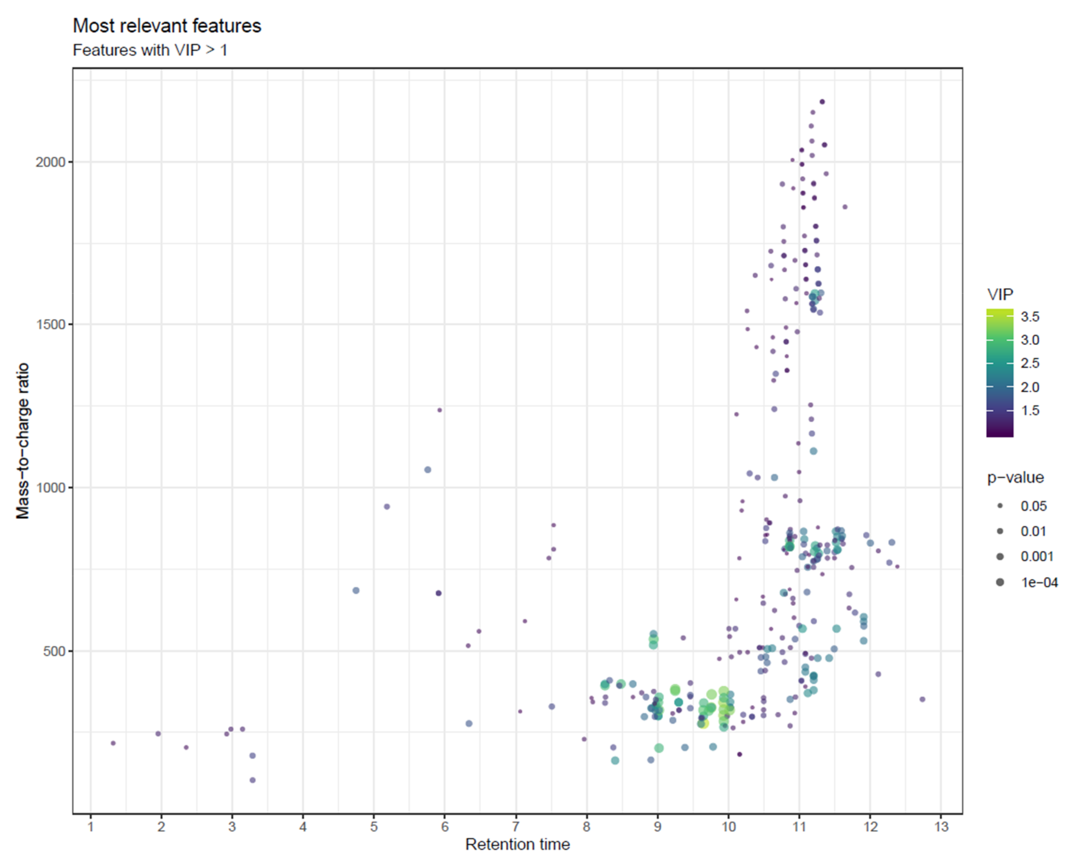
- To combine the information of both Manhattan plots, consider a scatter plot with m/z and retention time on the x- and y-axis, with the size of the point reflecting p-value and potentially colored by variable importance from multivariate modelling (e.g., VIP; Figure 24) or by effect size (e.g., fold change; not shown). While size is not an accurate metric in visualizations, this visualization combines mass and retention time so that the most interesting metabolite classes can be identified. As with Manhattan plots, these plots should be drawn separately for each column and ionization mode.
- 82.
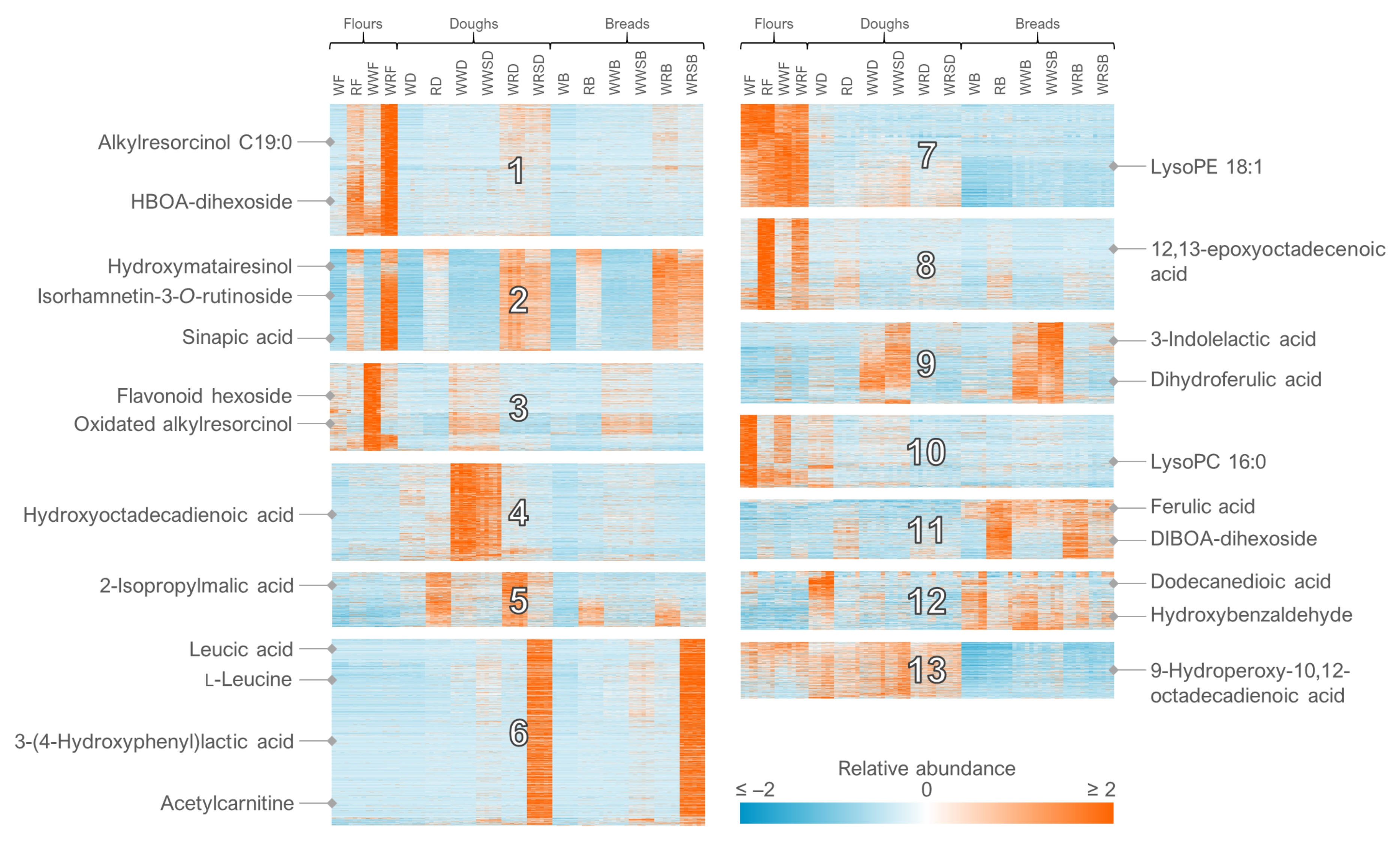
- For the clustering in Multiple Experiment Viewer, first normalize the rows (signal abundances) and select appropriate color scale limits for the normalized abundances (0 to 10% of features can be off limits). For hierarchical clustering, choose whether to cluster only the features or samples as well. Use Pearson correlation and average linkage clustering. For k-means clustering, choose cluster genes, use Pearson correlation, calculate k-means and choose a low number of clusters (e.g., 4) for the initial run. Repeat the procedure by increasing the number of clusters until no more clusters with a unique pattern emerge and choose the highest number of clusters based on this visual optimization.
3.5. Identification of Metabolites
3.5.1. Comparison with Pure Standard Compounds (MSI Level 1)
- 83.
- For the identification of metabolites (identification level 1 according to the Metabolomics Standards Initiative) [58], compare the molecular features against an in-house library (i.e., a reference standard analyzed previously with the same platform in the same chromatographic conditions). Apply the following criteria:
- a.
- matching m/z (within 10 ppm or according to instrument mass accuracy);
- b.
- similar retention time (ΔRT < 0.2–0.5 min), taking into consideration any possible near-eluting isomers.
- c.
- MS/MS spectra (main fragments matching within 0.02 Da in one or more CID voltage)
3.5.2. MS/MS Fragmentation and Database Comparison (MSI levels 2–3)
- 84.
- For the putative annotation of metabolites (ID level 2), compare the mol features against publicly available spectral databases, including a database file (compiled in MSP format for using within MS-DIAL) and online databases. The annotation has acceptable reliability if the main fragments (excluding the molecular ion) match between the experimental and reference MS/MS spectra in only one proposed metabolite. In case several alternatives exist with similar MS/MS, the common denominator of all the alternatives (e.g., a compound class, ID level 3) is given as the annotation instead. Apply the following criteria:
- a.
- matching m/z (within 10 ppm or according to instrument mass accuracy)
- b.
- MS/MS spectra (main fragments matching within 0.02 Da)
- 85.
- For the putative characterization of compound class (ID level 3), use the following approaches to obtain characteristic information of the metabolite:
- a.
- Compare the experimental MS/MS with in-silico generated spectra in MS-FINDER;
- b.
- Use the calculated molecular formula, retention time and diagnostic MS/MS fragments to determine the compound class.
3.5.3. Pathway Analysis
- 86.
- Option 1: In MetaboAnalyst [59] (https://www.metaboanalyst.ca/) use Enrichment or Pathway Analysis which enables enrichment and visualization of metabolic pathways in which the metabolites could potentially be involved. For more detailed information about metabolic regulation, the Network Explorer enables inclusion of fold change data, along with gene expression data.
- 87.
- Option 2: Cytoscape [60] (https://cytoscape.org/) is a powerful stand-alone tool that is used by biomedical researchers to visualize and dynamically analyze gene/protein/metabolite interaction networks. The strength of Cytoscape is even more apparent when linked to databases, e.g., MetScape [61], which allows for visualizing and interpreting metabolomic data in the context of human metabolic networks.
3.6. Biological Interpretation of the Results
4. Conclusions
Supplementary Materials
Author Contributions
Funding
Acknowledgments
Conflicts of Interest
References
- Johnson, C.H.; Ivanisevic, J.; Siuzdak, G. Metabolomics: Beyond biomarkers and towards mechanisms. Nat. Rev. Mol. Cell Biol. 2016, 17, 451–459. [Google Scholar] [CrossRef] [Green Version]
- Manach, C.; Hubert, J.; Llorach, R.; Scalbert, A. The complex links between dietary phytochemicals and human health deciphered by metabolomics. Mol. Nutr. Food Res. 2009, 53, 1303–1315. [Google Scholar] [CrossRef] [PubMed]
- Gika, H.; Virgiliou, C.; Theodoridis, G.; Plumb, R.S.; Wilson, I.D. Untargeted LC/MS-based metabolic phenotyping (metabonomics/metabolomics): The state of the art. J. Chromatogr. 2019, 1117, 136–147. [Google Scholar] [CrossRef]
- Nash, W.J.; Dunn, W.B. From mass to metabolite in human untargeted metabolomics: Recent advances in annotation of metabolites applying liquid chromatography-mass spectrometry data. TrAC Trends Anal. Chem. 2019, 120, 115324. [Google Scholar] [CrossRef]
- Johnson, C.H.; Ivanisevic, J.; Benton, H.P.; Siuzdak, G. Bioinformatics: The Next Frontier of Metabolomics. Anal. Chem. 2015, 87, 147–156. [Google Scholar] [CrossRef] [Green Version]
- Chaleckis, R.; Meister, I.; Zhang, P.; Wheelock, C.E. Challenges, progress and promises of metabolite annotation for LC–MS-based metabolomics. Curr. Opin. Biotechnol. 2019, 55, 44–50. [Google Scholar] [CrossRef] [PubMed]
- Misra, B.B.; Mohapatra, S. Tools and resources for metabolomics research community: A 2017–2018 update. Electrophoresis 2019, 40, 227–246. [Google Scholar] [CrossRef]
- Dias, D.A.; Jones, O.A.H.; Beale, D.J.; Boughton, B.A.; Benheim, D.; Kouremenos, K.A.; Wolfender, J.; Wishart, D.S. Current and future perspectives on the structural identification of small molecules in biological systems. Metabolites 2016, 6, 46. [Google Scholar] [CrossRef]
- Ulaszewska, M.M.; Weinert, C.H.; Trimigno, A.; Portmann, R.; Lacueva, C.A.; Badertscher, R.; Brennan, L.; Brunius, C.; Bub, A.; Capozzi, F.; et al. Nutrimetabolomics: An Integrative Action for Metabolomic Analyses in Human Nutritional Studies. Mol. Nutr. Food Res. 2019, 63, 1800384. [Google Scholar] [CrossRef]
- Broadhurst, D.; Goodacre, R.; Reinke, S.N.; Kuligowski, J.; Wilson, I.D.; Lewis, M.R.; Dunn, W.B. Guidelines and considerations for the use of system suitability and quality control samples in mass spectrometry assays applied in untargeted clinical metabolomic studies. Metabolomics 2018, 14, 72. [Google Scholar] [CrossRef] [Green Version]
- Koistinen, V.M.; Hanhineva, K. Microbial and endogenous metabolic conversions of rye phytochemicals. Mol. Nutr. Food Res. 2017, 61, 1600627. [Google Scholar] [CrossRef] [PubMed]
- Koistinen, V.M.; Hanhineva, K. Mass spectrometry-based analysis of whole-grain phytochemicals. Crit. Rev. Food Sci. Nutr. 2017, 57, 1688–1709. [Google Scholar] [CrossRef] [PubMed]
- De Mello, V.D.; Paananen, J.; Lindström, J.; Lankinen, M.A.; Shi, L.; Kuusisto, J.; Pihlajamäki, J.; Auriola, S.; Lehtonen, M.; Rolandsson, O.; et al. Indolepropionic acid and novel lipid metabolites are associated with a lower risk of type 2 diabetes in the Finnish Diabetes Prevention Study. Sci. Rep. 2017, 7, 46337. [Google Scholar] [CrossRef] [PubMed]
- Noerman, S.; Kärkkäinen, O.; Mattsson, A.; Paananen, J.; Lehtonen, M.; Nurmi, T.; Tuomainen, T.; Voutilainen, S.; Hanhineva, K.; Virtanen, J.K. Metabolic Profiling of High Egg Consumption and the Associated Lower Risk of Type 2 Diabetes in Middle-Aged Finnish Men. Mol. Nutr. Food Res. 2019, 63, 1800605. [Google Scholar] [CrossRef]
- Rothwell, J.A.; Keski-Rahkonen, P.; Robinot, N.; Assi, N.; Casagrande, C.; Jenab, M.; Ferrari, P.; Boutron-Ruault, M.; Mahamat-Saleh, Y.; Mancini, F.R.; et al. A Metabolomic Study of Biomarkers of Habitual Coffee Intake in Four European Countries. Mol. Nutr. Food Res. 2019, 63, 1900659. [Google Scholar] [CrossRef]
- Brunius, C.; Shi, L.; Landberg, R. Large-scale untargeted LC-MS metabolomics data correction using between-batch feature alignment and cluster-based within-batch signal intensity drift correction. Metabolomics 2016, 12, 173. [Google Scholar] [CrossRef] [Green Version]
- Tsugawa, H.; Cajka, T.; Kind, T.; Ma, Y.; Higgins, B.; Ikeda, K.; Kanazawa, M.; VanderGheynst, J.; Fiehn, O.; Arita, M. MS-DIAL: Data-independent MS/MS deconvolution for comprehensive metabolome analysis. Nat. Methods 2015, 12, 523–526. [Google Scholar] [CrossRef]
- Tsugawa, H.; Kind, T.; Nakabayashi, R.; Yukihira, D.; Tanaka, W.; Cajka, T.; Saito, K.; Fiehn, O.; Arita, M. Hydrogen Rearrangement Rules: Computational MS/MS Fragmentation and Structure Elucidation Using MS-FINDER Software. Anal. Chem. 2016, 88, 7946–7958. [Google Scholar] [CrossRef]
- R: The R Project for Statistical Computing. Available online: https://www.r-project.org/ (accessed on 19 December 2019).
- Agilent Technologies Agilent 6500 Series Q-TOF LC/MS system Maintenance Guide Research Use Only. Not for use in Diagnostic Procedures. Available online: https://www.crawfordscientific.com/media/wysiwyg/Literature/CMS/Tech_Pages/Agilent_Maintenance_Docs/6500%20Series%20QTOF/6500_Q-TOF_Maintenance%20Guide.pdf (accessed on 30 March 2020).
- Certificate of Analysis API-TOF Reference Mass Solution Kit Agilent Part Number: G1969-85001. Available online: https://www.agilent.com/cs/library/certificateofanalysis/G1969-85001cofa872024U-LB25990.pdf (accessed on 30 March 2020).
- Chang, W.; Cheng, J.; Allaire, J.J.; Xie, Y.; McPherson, J.; RStudio; jQuery Foundation; jQuery contributors; jQuery UI contributors; Otto, M.; et al. shiny: Web Application Framework for R. R package version 1.2.0. Available online: https://CRAN.R-project.org/package=shiny (accessed on 30 March 2020).
- Kirwan, J.A.; Broadhurst, D.I.; Davidson, R.L.; Viant, M.R. Characterising and correcting batch variation in an automated direct infusion mass spectrometry (DIMS) metabolomics workflow. Anal. Bioanal. Chem. 2013, 405, 5147–5157. [Google Scholar] [CrossRef]
- R: Fit a Smoothing Spline. Available online: https://stat.ethz.ch/R-manual/R-devel/library/stats/html/smooth.spline.html (accessed on 30 March 2020).
- Puupponen-Pimiä, R.; Seppänen-Laakso, T.; Kankainen, M.; Maukonen, J.; Törrönen, R.; Kolehmainen, M.; Leppänen, T.; Moilanen, E.; Nohynek, L.; Aura, A.-M.; et al. Effects of ellagitannin-rich berries on blood lipids, gut microbiota, and urolithin production in human subjects with symptoms of metabolic syndrome. Mol. Nutr. Food Res. 2013, 57, 2258–2263. [Google Scholar] [CrossRef]
- Breheny, P.; Stromberg, A.; Lambert, J. P-Value histograms: Inference and diagnostics. High-Throughput 2018, 7, 23. [Google Scholar] [CrossRef] [PubMed] [Green Version]
- Hotelling, H. Relations Between Two Sets of Variates. Biometrika 1936, 28, 321. [Google Scholar] [CrossRef]
- Bro, R.; Smilde, A.K. Principal component analysis. Anal. Methods 2014, 6, 2812–2831. [Google Scholar] [CrossRef] [Green Version]
- Pearson, K. LIII. On lines and planes of closest fit to systems of points in space. London Edinburgh Dublin Philos. Mag. J. Sci. 1901, 2, 559–572. [Google Scholar] [CrossRef] [Green Version]
- van der Maaten, L.; Hinton, G. Visualizing Data using t-SNE. J. Mach. Learn. Res. 2008, 9, 2579–2605. [Google Scholar]
- Rokach, L.; Maimon, O. Clustering Methods. In Data Mining and Knowledge Discovery Handbook; Springer: New York, NY, USA, 2005; pp. 321–352. [Google Scholar]
- Murtagh, F.; Legendre, P. Ward’s Hierarchical Agglomerative Clustering Method: Which Algorithms Implement Ward’s Criterion? J. Classif. 2014, 31, 274–295. [Google Scholar] [CrossRef] [Green Version]
- Kokla, M.; Virtanen, J.; Kolehmainen, M.; Paananen, J.; Hanhineva, K. Random forest-based imputation outperforms other methods for imputing LC-MS metabolomics data: A comparative study. BMC Bioinform. 2019, 20, 1–11. [Google Scholar] [CrossRef] [Green Version]
- Stekhoven, D.J.; Bühlmann, P. Data and text mining MissForest-non-parametric missing value imputation for mixed-type data. Bioinformatics 2012, 28, 112–118. [Google Scholar] [CrossRef] [Green Version]
- Armitage, E.G.; Godzien, J.; Alonso-Herranz, V.; López-Gonzálvez, Á.; Barbas, C. Missing value imputation strategies for metabolomics data. Electrophoresis 2015, 36, 3050–3060. [Google Scholar] [CrossRef]
- Beretta, L.; Santaniello, A. Nearest neighbor imputation algorithms: A critical evaluation. BMC Med. Inform. Decis. Mak. 2016, 16, 74. [Google Scholar] [CrossRef] [Green Version]
- Sysi-Aho, M.; Katajamaa, M.; Yetukuri, L.; Orešič, M. Normalization method for metabolomics data using optimal selection of multiple internal standards. BMC Bioinform. 2007, 8, 93. [Google Scholar] [CrossRef] [PubMed] [Green Version]
- di Guida, R.; Engel, J.; Allwood, J.W.; Weber, R.J.M.; Jones, M.R.; Sommer, U.; Viant, M.R.; Dunn, W.B. Non-targeted UHPLC-MS metabolomic data processing methods: A comparative investigation of normalisation, missing value imputation, transformation and scaling. Metabolomics 2016, 12, 93. [Google Scholar] [CrossRef] [PubMed] [Green Version]
- Kohl, S.M.; Klein, M.S.; Hochrein, J.; Oefner, P.J.; Spang, R.; Gronwald, W. State-of-the art data normalization methods improve NMR-based metabolomic analysis. Metabolomics 2012, 8, 146–160. [Google Scholar] [CrossRef] [PubMed] [Green Version]
- Tyralis, H.; Papacharalampous, G.; Langousis, A. A Brief Review of Random Forests for Water Scientists and Practitioners and Their Recent History in Water Resources. Water 2019, 11, 910. [Google Scholar] [CrossRef] [Green Version]
- Mattsson, A. Analysis of LC-MS Data in Untargeted Nutritional Metabolomics. Master’s Thesis, Aalto University, Espoo, Finland, August 2019. Available online: https://aaltodoc.aalto.fi/handle/123456789/39870 (accessed on 31 March 2020).
- Senan, O.; Aguilar-Mogas, A.; Navarro, M.; Capellades, J.; Noon, L.; Burks, D.; Yanes, O.; Guimerà, R.; Sales-Pardo, M. CliqueMS: A computational tool for annotating in-source metabolite ions from LC-MS untargeted metabolomics data based on a coelution similarity network. Bioinformatics 2019, 35, 4089–4097. [Google Scholar] [CrossRef] [Green Version]
- Kachman, M.; Habra, H.; Duren, W.; Wigginton, J.; Sajjakulnukit, P.; Michailidis, G.; Burant, C.; Karnovsky, A. Deep annotation of untargeted LC-MS metabolomics data with Binner. Bioinformatics 2020, 36, 1801–1806. [Google Scholar] [CrossRef]
- Kouřil, Š.; de Sousa, J.; Václavík, J.; Friedecký, D.; Adam, T. CROP: Correlation-based reduction of feature multiplicities in untargeted metabolomic data. Bioinformatics 2020. [Google Scholar] [CrossRef]
- Vinaixa, M.; Samino, S.; Saez, I.; Duran, J.; Guinovart, J.J.; Yanes, O. A Guideline to Univariate Statistical Analysis for LC/MS-Based Untargeted Metabolomics-Derived Data. Metabolites 2012, 2, 775–795. [Google Scholar] [CrossRef]
- Kuznetsova, A.; Brockhoff, P.B.; Christensen, R.H.B. lmerTest Package: Tests in Linear Mixed Effects Models. J. Stat. Softw. 2017, 82. [Google Scholar] [CrossRef] [Green Version]
- Bates, D.; Mächler, M.; Bolker, B.; Walker, S. Fitting Linear Mixed-Effects Models using lme4. arXiv 2014, arXiv:1406.5823. Available online: https://arxiv.org/abs/1406.5823 (accessed on 30 March 2020).
- Claggett, B.L.; Antonelli, J.; Henglin, M.; Watrous, J.D.; Lehmann, K.A.; Musso, G.; Correia, A.; Jonnalagadda, S.; Demler, O.V.; Vasan, R.S.; et al. Quantitative Comparison of Statistical Methods for Analyzing Human Metabolomics Data. arXiv 2017, arXiv:1710.03443. Available online: https://arxiv.org/abs/1710.03443 (accessed on 30 March 2020).
- Stoessel, D.; Stellmann, J.; Willing, A.; Behrens, B.; Rosenkranz, S.C.; Hodecker, S.C.; Stürner, K.H.; Reinhardt, S.; Fleischer, S.; Deuschle, C.; et al. Metabolomic Profiles for Primary Progressive Multiple Sclerosis Stratification and Disease Course Monitoring. Front. Hum. Neurosci. 2018, 12, 226. [Google Scholar] [CrossRef] [PubMed]
- Shi, L.; Westerhuis, J.A.; Rosén, J.; Landberg, R.; Brunius, C. Variable selection and validation in multivariate modelling. Bioinformatics 2019, 35, 972–980. [Google Scholar] [CrossRef] [PubMed]
- Breiman, L.; Cutler, A. Random Forests. Mach. Learn. 2001, 45, 5–32. [Google Scholar] [CrossRef] [Green Version]
- Smith, C.A.; Maille, G.O.; Want, E.J.; Qin, C.; Trauger, S.A.; Brandon, T.R.; Custodio, D.E.; Abagyan, R.; Siuzdak, G. METLIN: A metabolite mass spectral database. Ther. Drug Monit. 2005, 27, 747–751. [Google Scholar] [CrossRef]
- Horai, H.; Arita, M.; Kanaya, S.; Nihei, Y.; Ikeda, T.; Suwa, K.; Ojima, Y.; Tanaka, K.; Tanaka, S.; Aoshima, K.; et al. MassBank: A public repository for sharing mass spectral data for life sciences. J. Mass Spectrom. 2010, 45, 703–714. [Google Scholar] [CrossRef]
- Afendi, F.M.; Okada, T.; Yamazaki, M.; Hirai-Morita, A.; Nakamura, Y.; Nakamura, K.; Ikeda, S.; Takahashi, H.; Altaf-Ul-Amin, M.; Darusman, L.K.; et al. KNApSAcK Family Databases: Integrated Metabolite–Plant Species Databases for Multifaceted Plant Research. Plant Cell Physiol. 2012, 53, e1. [Google Scholar] [CrossRef] [Green Version]
- Wishart, D.S.; Jewison, T.; Guo, A.C.; Wilson, M.; Knox, C.; Liu, Y.; Djoumbou, Y.; Mandal, R.; Aziat, F.; Dong, E.; et al. HMDB 3.0—The Human Metabolome Database in 2013. Nucleic Acids Res. 2012, 41, D801–D807. [Google Scholar] [CrossRef]
- MassBank of North America. Available online: https://mona.fiehnlab.ucdavis.edu/ (accessed on 8 October 2019).
- Fahy, E.; Sud, M.; Cotter, D.; Subramaniam, S. LIPID MAPS online tools for lipid research. Nucleic Acids Res. 2007, 35, W606–W612. [Google Scholar] [CrossRef] [PubMed] [Green Version]
- Sumner, L.W.; Amberg, A.; Barrett, D.; Beale, M.H.; Beger, R.; Daykin, C.A.; Fan, T.W.-M.; Fiehn, O.; Goodacre, R.; Griffin, J.L.; et al. Proposed minimum reporting standards for chemical analysis. Metabolomics 2007, 3, 211–221. [Google Scholar] [CrossRef] [PubMed] [Green Version]
- Chong, J.; Yamamoto, M.; Xia, J. MetaboAnalystR 2.0: From Raw Spectra to Biological Insights. Metabolites 2019, 9, 57. [Google Scholar] [CrossRef] [PubMed] [Green Version]
- Shannon, P.; Markiel, A.; Ozier, O.; Baliga, N.S.; Wang, J.T.; Ramage, D.; Amin, N.; Schwikowski, B.; Ideker, T. Cytoscape: A software Environment for integrated models of biomolecular interaction networks. Genome Res. 2003, 13, 2498–2504. [Google Scholar] [CrossRef]
- Gao, J.; Tarcea, V.G.; Karnovsky, A.; Mirel, B.R.; Weymouth, T.E.; Beecher, C.W.; Cavalcoli, J.D.; Athey, B.D.; Omenn, G.S.; Burant, C.F.; et al. Metscape: A Cytoscape plug-in for visualizing and interpreting metabolomic data in the context of human metabolic networks. Bioinformatics. 2010, 26, 971–973. [Google Scholar] [CrossRef] [PubMed] [Green Version]
- Kärkkäinen, O.; Lankinen, M.A.; Vitale, M.; Jokkala, J.; Leppänen, J.; Koistinen, V.; Lehtonen, M.; Giacco, R.; Rosa-Sibakov, N.; Micard, V.; et al. Diets rich in whole grains increase betainized compounds associated with glucose metabolism. Am. J. Clin. Nutr. 2018, 108, 971–979. [Google Scholar] [CrossRef] [PubMed] [Green Version]
- Tuomainen, M.; Kärkkäinen, O.; Leppänen, J.; Auriola, S.; Lehtonen, M.; Savolainen, M.J.; Hermansen, K.; Risérus, U.; Åkesson, B.; Thorsdottir, I.; et al. Quantitative assessment of betainized compounds and associations with dietary and metabolic biomarkers in the randomized study of the healthy Nordic diet (SYSDIET). Am. J. Clin. Nutr. 2019, 110, 1108–1118. [Google Scholar] [CrossRef]


© 2020 by the authors. Licensee MDPI, Basel, Switzerland. This article is an open access article distributed under the terms and conditions of the Creative Commons Attribution (CC BY) license (http://creativecommons.org/licenses/by/4.0/).
Share and Cite
Klåvus, A.; Kokla, M.; Noerman, S.; Koistinen, V.M.; Tuomainen, M.; Zarei, I.; Meuronen, T.; Häkkinen, M.R.; Rummukainen, S.; Farizah Babu, A.; et al. “Notame”: Workflow for Non-Targeted LC–MS Metabolic Profiling. Metabolites 2020, 10, 135. https://doi.org/10.3390/metabo10040135
Klåvus A, Kokla M, Noerman S, Koistinen VM, Tuomainen M, Zarei I, Meuronen T, Häkkinen MR, Rummukainen S, Farizah Babu A, et al. “Notame”: Workflow for Non-Targeted LC–MS Metabolic Profiling. Metabolites. 2020; 10(4):135. https://doi.org/10.3390/metabo10040135
Chicago/Turabian StyleKlåvus, Anton, Marietta Kokla, Stefania Noerman, Ville M. Koistinen, Marjo Tuomainen, Iman Zarei, Topi Meuronen, Merja R. Häkkinen, Soile Rummukainen, Ambrin Farizah Babu, and et al. 2020. "“Notame”: Workflow for Non-Targeted LC–MS Metabolic Profiling" Metabolites 10, no. 4: 135. https://doi.org/10.3390/metabo10040135