A Stochastic Interpolation-Based Fractal Model for Vulnerability Diagnosis of Water Supply Networks Against Seismic Hazards

Abstract

Historical seismic events show that water supply networks are increasingly vulnerable to seismic damage, especially in a violent earthquake, which leads to an unprecedented level of risk. Evaluation of vulnerability to seismic hazards can be considered as one of the first steps of risk management and mitigation. This paper presents a stochastic interpolation-based fractal model for assessing the physical vulnerability of urban water supply pipelines. Firstly, based on the formation mechanism of natural disaster risk and the concept of seismic vulnerability, the most representative factors were selected as the vulnerability evaluation indices, and the classification criterion of each index was teased out according to the earthquake damage investigations and researches on the aseismatic behavior of water supply pipelines. Secondly, considering the randomness of vulnerability to earthquake hazards, the test data set was produced by way of stochastic interpolation according to the uniform distribution, on the basis of the classification criterion. The fractal dimensions of all of the indices were calculated based on the test data set. The fractal interpolation diagnosis function for identifying the vulnerability levels of pipelines to earthquake disasters was established. Finally, the application of the proposed model to a real water supply network and its comparative analysis showed that the water supply network was basically in a medium vulnerability level. Through the case study verification, we could find that the model was theoretically and practically feasible. This study helps to gain a better understanding of the extents of potential vulnerability levels of water supply pipelines. It can provide technical support for disaster prevention plans of urban water supply networks.

1. Introduction

The water supply network (WSN) is an important facility of urban lifeline systems. It not only provides daily water for people, but also meets the emergency functional requirements during disasters, such as the water for emergency medical refuge evacuation, fire relief, etc. [1,2]. An urban WSN composed of many nodes and pipelines is widely distributed in the city [3,4]. Given their spatial distributions, WSNs may be subjected to different seismic effects. Recent events proved that urban water supply networks are becoming increasingly vulnerable to earthquake damage; it is alarming that once water supply pipes are damaged, people's work and living will suffer great inconvenience, emergency rescues will be impeded, and post-earthquake fires will produce amplification effects owing to the loss of emergency service function of the water supply pipes [5,6,7,8], as shown during events in the USA (San Fernando, 1971; Northridge, 1994), Japan (Kobe, 1995; East Japan, 2011), China (Wenchuan, 2008; Lushan, 2013), and Nepal (2015). Since seismic hazard cannot generally be diminished, the vulnerability is one aspect where efforts can be expended with the goal of disaster risk reduction [9]. Hence, understanding and being able to measure the vulnerability of water supply pipes are the key factors in managing disaster risk. Accurate diagnosis and management of these vulnerable parts of the WSN are required, which can provide the basis for identifying weak points of the urban WSN and putting forward disaster prevention countermeasures in a targeted manner.

Previous researches on water supply networks have been performed in the aspects that follow: (1) Seismic response and seismic reliability of buried water pipelines [10,11,12]; (2) seismic connectivity reliability, hydraulic function reliability, and seismic service performance [13,14]; (3) performance-based seismic design [15,16]; (4) post-earthquake function recovery [17,18,19,20]. The above aspects belong to seismic performance research or optimal design of the WSN in earthquake scenarios, which are carried out by the way of theoretical calculation, numerical simulation, and intelligent optimization algorithms [10,20,21], taking external environments (i.e., seismic hazard and site types) and structural attributes of pipes into account. In reality, however, the information that we obtain is incomplete, and the earthquake or the site condition also has highly random characteristics. These methods proposed above are not very practical in urban earthquake disaster prevention plans. Recently, more and more attention has been focused on either vulnerability analysis or risk assessment of water supply pipelines [2,22,23,24]. Since WSNs are naturally vulnerable to physical threats, particularly during earthquake events, a novel vulnerability assessment tool is useful for identifying the vulnerable components of a WSN during an earthquake.

Bai [25] and Wu et al. [26] established a vulnerability assessment index system of water supply pipes exposed to seismic hazards based on the structure characteristics of pipes and built a theory-based catastrophe model. However, the site condition was not taken into account, and the vulnerability index weights in the model needed to be determined by a human. As a consequence, there was great subjectivity in the model. Wang et al. [27] developed a node-importance-based method for assessing the vulnerability of the WSN. The method conducted a vulnerability analysis from the whole network perspective. It could not list the special weak pipes. Halfaya et al. [28] proposed a vulnerability index for pipes, taking into account the main parameters governing their vulnerability. Through a comparative analysis of the vulnerability index, the weak parts of the WSN would be identified regardless of the occurrence probability of earthquakes. Obviously, the studies above developed a vulnerability assessment system to evaluate the seismic vulnerability level of water supply pipelines from the structure property perspective. However, soil characteristics are also the key elements for the occurrence of seismic damage on individual mains, together with the earthquake magnitude [2,29]. Therefore, the concept of seismic vulnerability and its constituent elements is presented in this study based on the disaster formation process and the formation mechanism of disaster risk. This paper attempts to develop a seismic vulnerability index system and respectively tease out the quantitative relationship between the vulnerability level of the pipes and the vulnerability indices. Considering the randomness and nonlinearity between vulnerability indices and the vulnerability level of the pipes, this paper developed a stochastic interpolation-based fractal model for vulnerability diagnosis of water supply pipes, and the model was applied in a WSN of a city in South China.

2. Seismic Vulnerability of WSN and Its Modeling Method

2.1. The Basic Concept of Seismic Vulnerability of the WSN

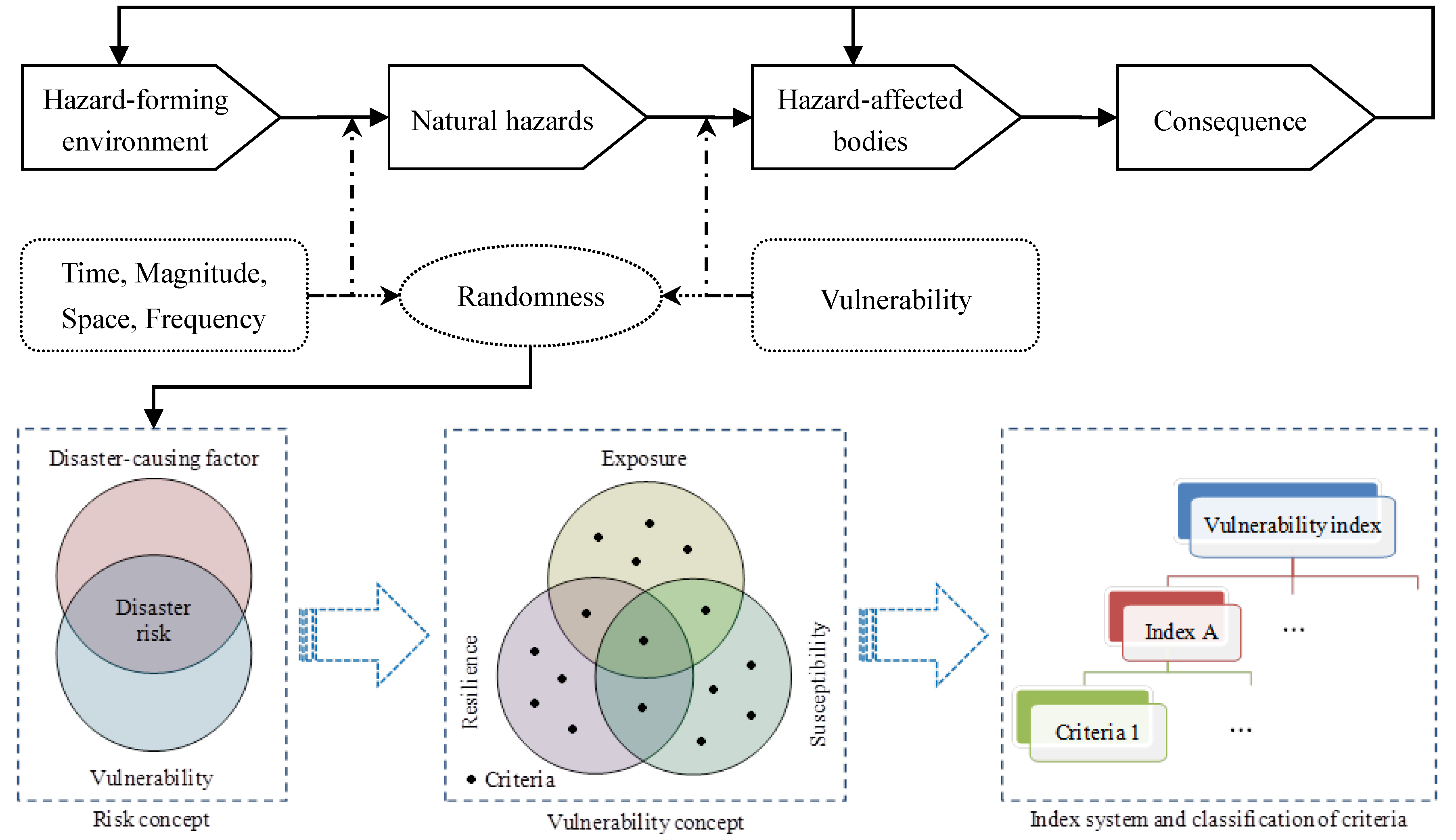
A conceptual model for seismic vulnerability assessment of the WSN is shown in Figure 1, based on the disaster formation process [30,31,32] and disaster risk formation mechanism [33,34,35]. Natural hazards are the natural events that arise from the hazard-forming environment (that is, a specific geophysical environment), accompanied by concentrations of energy released to produce major threats to human life or economic assets [36,37]. Space, time, magnitude, and frequency are the basic characteristics of natural hazards, i.e., the disaster-causing factors. They are determined by the hazard-forming environment [38,39]. Hazard-affected bodies are defined as people, substances, and environments that are under the threat from natural hazards. The natural hazards’ interaction with hazard-affected bodies can result in losses and impacts of a human, material, economic, and environmental nature [40]. The induced consequences also influence the hazard-forming environment and the hazard-affected bodies.

Both natural hazards and the vulnerability of hazard-affected bodies have the characteristics of randomness. Risk develops through interactions of disaster-causing factors and vulnerability of hazard-affected bodies [33,34,35], as shown in Figure 1. Vulnerability is naturally born of the risk. It is an inherent attribute of hazard-affected bodies, and it reflects the impact of natural hazards on hazard-affected bodies. The vulnerability varies with the disaster-causing factors. Generally, the distribution of a WSN is given in urban planning, while an earthquake happens with indeterminacy. We cannot eliminate or change the earthquake, but we can reduce the vulnerability of the WSN step by step for risk reduction. So, we take the WSN as the hazard-affected body when a quake occurs, the disaster-causing factor is the earthquake, and the vulnerability refers to the possibility for earthquake damage of pipes [41]. The WSN is vulnerable to earthquakes due to three main factors: Exposure, susceptibility, and resilience [42], as shown in Figure 1. Exposure refers to the spatial distribution of the WSN. Resilience has been defined as the ability of pipelines exposed to hazards to resist, absorb, accommodate to, and recover from the effects of a hazard in a timely and efficient manner, including the preservation and restoration of a WSN’s essential basic structures and functions [43]. Susceptibility is defined in terms of the elements exposed within the system, which influence the probabilities of being harmed in earthquake [44]. Vulnerability is the intersection of the three aspects. Hence, the vulnerability assessment model will contain indices from the three aspects, and mainly reflect the sensitivity and resilience of pipes at risk. The model also incorporates the criteria of vulnerability level of all of the indices to provide an easy way to ascertain the vulnerability to earthquake hazards such that adaptive and mitigation strategies can easily be defined and applied to drivers of high vulnerability [45].

Given the above, suppose that the WSN is subjected to the same seismic action. The representative indices of vulnerability to earthquake hazards, which cover the mentioned aspects, are elected. In addition, an assessment method is defined around a main axis that is formed by the vulnerability indices, which include criteria. The first step of seismic vulnerability assessment is to select appropriate criteria and classify them under different indices, as shown in Figure 1.

2.2. Analysis of Indices: Searching for the Relationships between Indices and Vulnerability

To practically evaluate the vulnerability levels of water supply pipelines, it is of utmost importance to identify the factors that make water supply pipelines vulnerable to earthquakes and to explore how these factors take effect. Thus, a list of the main influencing factors and the grade criteria of vulnerability should be identified firstly based on earthquake damage statistics and characteristics of water supply pipes. The earthquake damage survey data show that urban water supply pipes mainly have several failure modes under seismic action, such as the fracture failure of pipes, joint failure of pipes, and the connection failure between tee joints, elbows, valves, and pipes. The damage of buried pipelines by earthquakes is caused by multiple factors in common, and the mechanism of failure is rather complex. In accordance with earthquake damage survey data and mechanism researches on the seismic performance of pipes, the vulnerability of pipes is mainly determined by pipe material, pipe diameter, joint type, pipe age, thickness of covering soil, and site classification.

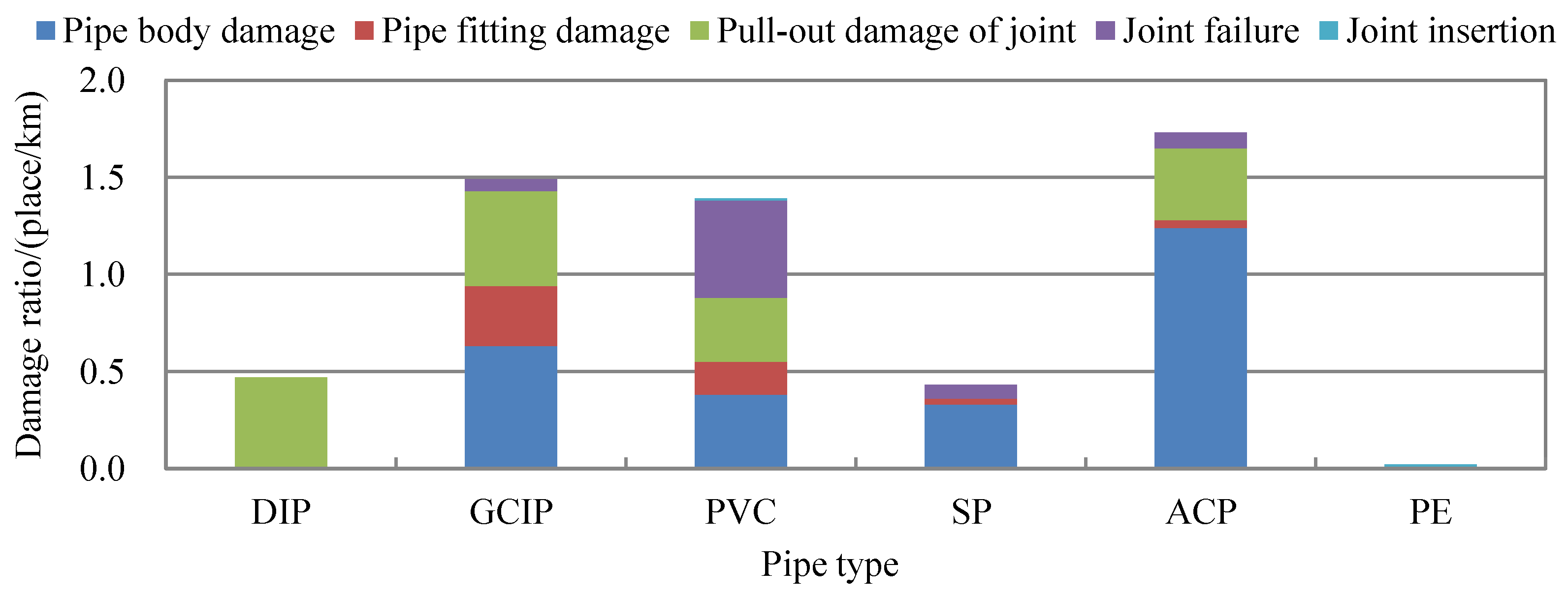
During an earthquake, a pipe made of rigid materials is severely destroyed, but the damage to a pipe made of flexible materials is slight. The damage conditions of pipes in the Kobe earthquake [46] are shown in Figure 2. The damaged pipes include ductile iron pipe (DIP), gray cast-iron pipe (GCIP), polyvinyl chloride pipe (PVC), steel pipe (SP), asbestos cement pipe (ACP), and polyethylene pipe (PE).

The reason for the serious destruction of PVC pipe is likely to be the low anti-seismic performance of PVC pipe due to its ageing. In the Wenchuan earthquake, the damage of pipes, from the serious level to light level, was as follows: Concrete pipe (especially self-prestressed concrete pipe, SPCP), GCIP, PVC, PE, DIP, and SP [47]. So, the seismic performance of a PE pipe and a steel–plastic composite pipe is the best, closely followed by SP, PVC pipe, and ductile CIP. The third level includes GCIP and SPCP. The concrete pipe, wrapped fiber reinforce plastic (FRP) pipe, and asbestos cement pipe are the worst.

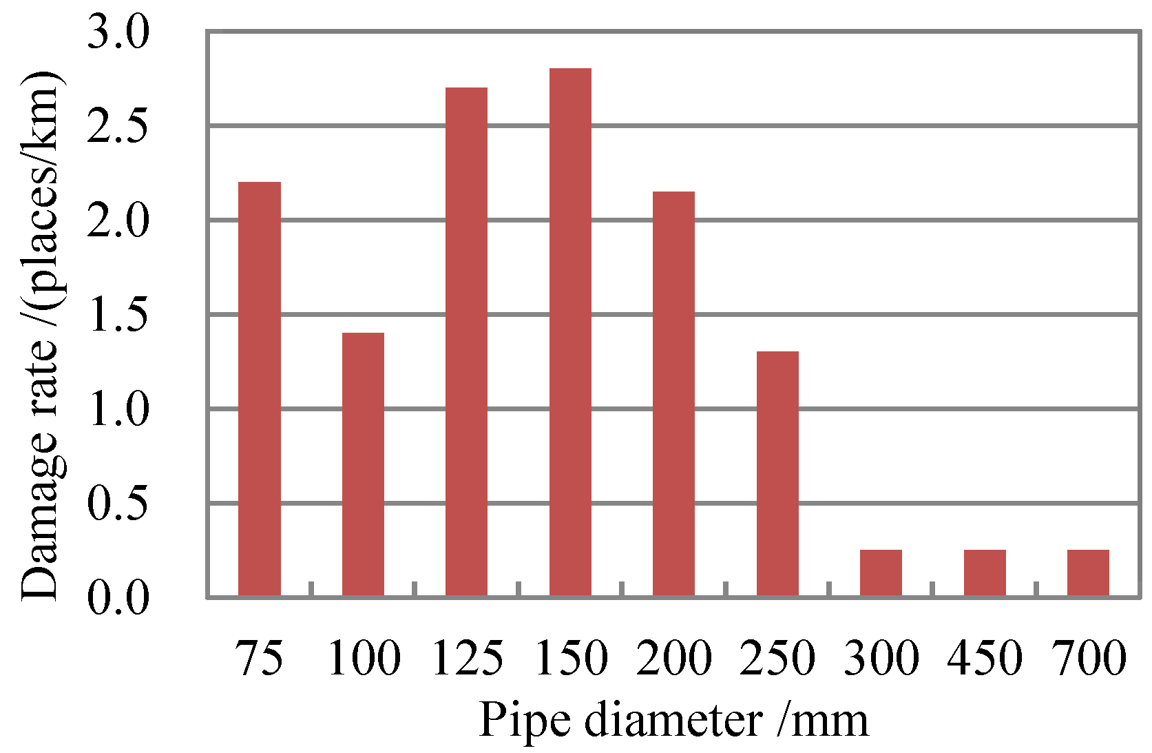
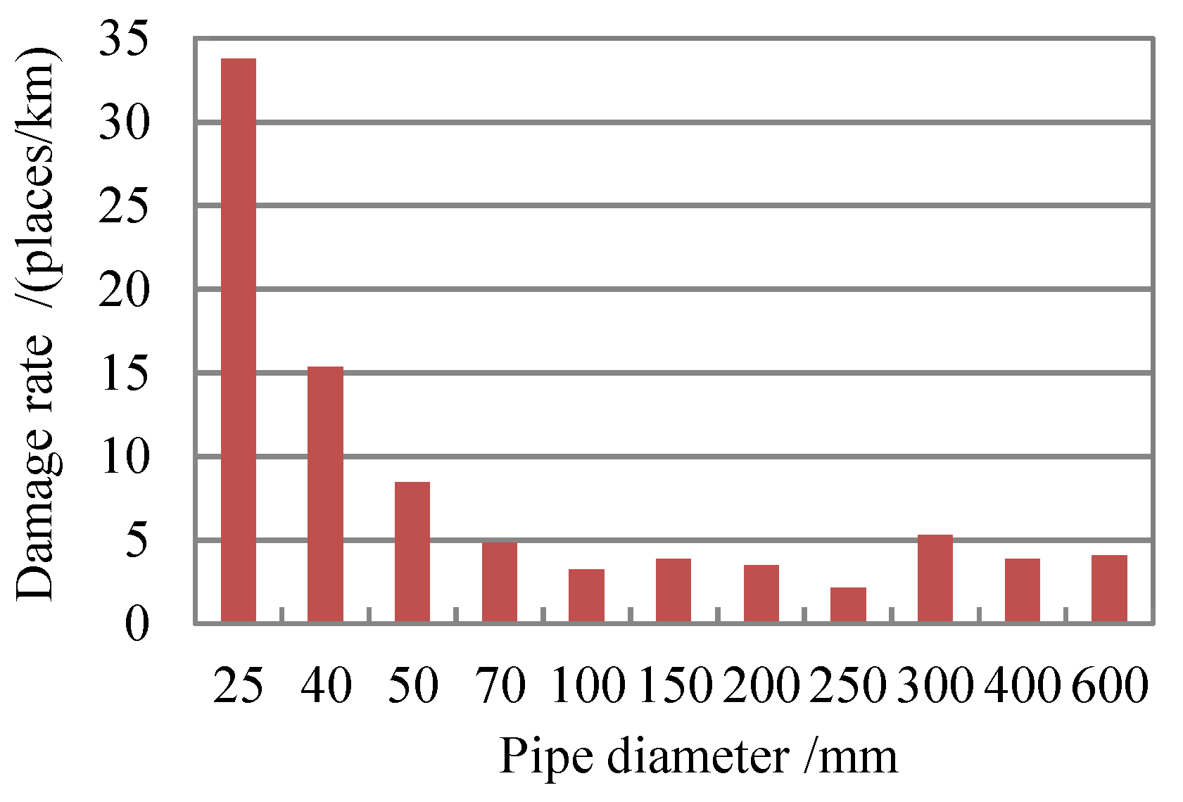
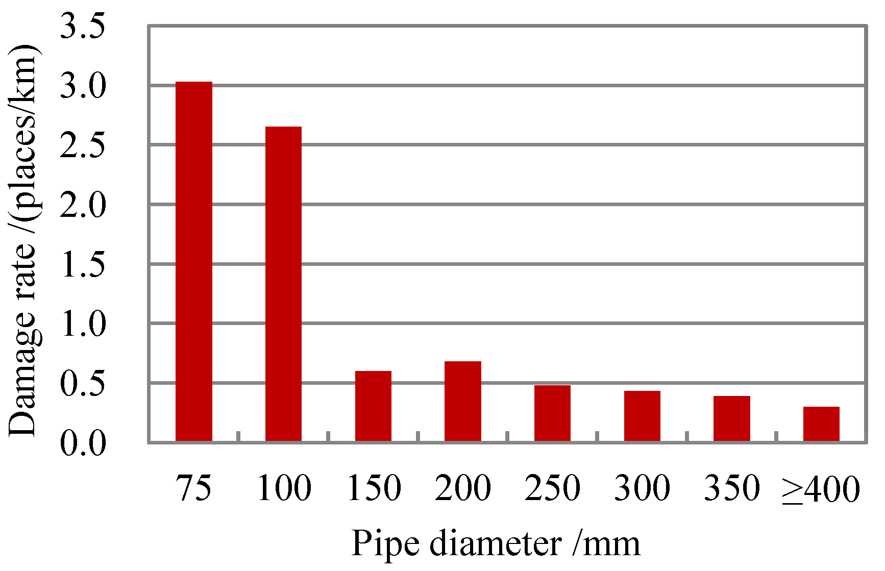
Earthquake damage data indicate that the stiffness of a pipe with small diameter and large slenderness ratio is relatively smaller, which has made it vulnerable to damage. The pipes with small diameters are seriously damaged, and the pipes with large diameters are lightly damaged. This phenomenon is basically consistent with the destruction law in the Kobe earthquake, Tangshan earthquake [48], and Haicheng earthquake [49], shown in Figure 3, Figure 4 and Figure 5. The damage rate of pipes decreases with increasing tube diameter. In the earthquake damage records, more than 80% of the pipes damaged were ones less than 200 mm in diameter.

The pipe joint is another factor influencing the anti-seismic performance of pipeline. Comparing with the strength of a pipe, the pipe joint is the weak point of pipelines for aseismatic performance. The historical earthquake damage indicates that the aseismic performance of a flexible joint is better than that of a rigid joint in similar circumstances. In earthquakes, an old pipe is more vulnerable to damage than a new one. The corrosion and aging makes the pipes more brittle, and the strength of the pipe declines, as well as its resilience. For instance, the damage to cast-iron pipes was almost induced from pipe aging in the Wenchuan earthquake [47]. With the increase of buried depth of a pipe, the earthquake damage to the pipe reduces, because the motion velocity and deformation of the earth layer will become smaller. In general, the earthquake damage of shallow-buried pipes is more severe than that of deep-buried pipes. For example, the sewage treatment pipes in Dujiangyan city, 150 mm in diameter and buried in 3 m deep, were pre-stressed concrete pipes. They were not destroyed in the Wenchuan earthquake [5].

The influence of site condition on pipeline damage is very large. Soft sites may be more easily destroyed during earthquakes, which will aggravate the earthquake damage of buried pipes. This phenomenon was verified in the Kanto earthquake, San Fernando earthquake, and Tangshan earthquake. The damage data of buried pipes distributed in different sites [47] are shown in

Table 1. Damage rates of pipes in different sites.

District	Seismic Intensity (Degree)	Soil Type of the Site	Damage Rate (Places/km)
Tianjin City	7–8	Type 3	0.18
Tanggu district	8	Type 3	4.18
Hangu district	9	Type 3	10.00
Tangshan city	10–11	Type 2	4.00
San Fernando	8	Type 1	0.09
Los Angeles	6	Type 2	0.62
Sendai area	9	Type 1	0.03
		Type 2	0.22
		Type 3	0.87

Note: 1. The geological conditions of the Tanggu district are worse than those of Tianjin city, and the geological conditions of the Hangu district are worse than those of the Tanggu district. 2. Soil types are divided into four types: Type 1, Type 2, Type 3, and Type 4. Type 1 soil refers to rock or compact gravel soil; Type 2 soil refers to loose gravel soil, coarse sand, and cohesive soil (allowable bearing capacity of foundation soil is greater than 150 kPa); Type 4 soil refers to mucky soil, silty sand, and filling soil (allowable bearing capacity of foundation soil is less than 130 kPa); others belong to Type 3 soil.

. They show that the damage of water supply pipelines in poor site conditions is more severe than that in good site conditions.

In this paper, we only consider the vulnerability of the WSN. Suppose that the seismic intensity acting on all the pipes is the same. Therefore, pipe material (x₁), pipe diameter (x₂), joint type (x₃), pipe age (x₄), site type (x₅), and thickness of covering soil (x₆) were chosen to establish the evaluation system of seismic vulnerability. Referring to the earthquake damage survey and some research achievements, four grades were taken into consideration for the vulnerability level and were described as very low, low, medium, or high. The range of each grade was summarized in

Table 2. Grading standards for seismic vulnerability assessment of water supply pipelines.

Grade	x1	x2 (mm)	x3	x4 (Year)	x5	x6 (m)
High (IV)	Wrapped FRP pipe Asbestos cement pipe Concrete pipe	x2 ≤ 200	Adhesion connection Threaded connection Asbestos cement Self-stressing cement	50 ≤ x4	Type 4	x6 ≤ 0.5
Medium (III)	Plain cast-iron pipe Prestressed reinforced concrete pipe	200 < x2 ≤ 500	Welding	30 ≤x4 < 50	Type 3	0.5 < x6 ≤ 1
Low (II)	Polyvinyl chloride pipe Steel pipe Ductile cast-iron pipe	500 < x2 ≤ 800	Hot-melt connection Flange connection	10 ≤ x4 < 30	Type 2	1 < x6 ≤ 2
Very low (I)	Polythene pipe Steel–plastic compound pipe	800 < x2	Rubber ring connection	x4 < 10	Type 1	2 < x6

.

2.3. Stochastic Interpolation-Based Fractal Model for Seismic Vulnerability Assessment of WSNs

Owing to the nonlinear relationship between each index and the vulnerability levels, where the randomness usually exists, cooperative phenomena, and coherent effects between all the indices, a novel method is needed to deal with the problem. While the fractal theory studies nonlinear science on the basis of the self-similarity property existing between the part and the whole, it reveals the rules behind nonlinear complex phenomena and internal relationships between the part and the whole through fractal dimension [27,50]. There are many factors influencing the seismic vulnerability levels of WSNs. The vulnerability level of a WSN has chaotic characteristics, i.e., fractal characteristics, because of the diversity of factors influencing the vulnerability. Therefore, the concept of fractal dimension is introduced into the seismic vulnerability assessment of the WSN. It can effectively represent the fractal characteristics of seismic vulnerability of the WSN. The fractal dimension of each index can be calculated according to the following steps:

(1) Quantization of qualitative indices. x₁, x₃, and x₅ are qualitative indices. For the convenience of computing, let the index take an integer between 1 and 4. The attribute values of the indices x₁, x₃, and x₅ are quantified as 4, 3, 2, and 1, respectively, according to the grade: High, medium, low, and very low. So, the grade interval classification is given in

Table 3. Grade interval classification for seismic vulnerability assessment.

Grade	x1	x2 (mm)	x3	x4 (Year)	x5	x6 (m)
High (IV)	3.5–4.5	0–200	3.5–4.5	50–70	3.5–4.5	0.0–0.5
Medium (III)	2.5–3.5	200–500	2.5–3.5	30–50	2.5–3.5	0.5–1.0
Low (II)	1.5–2.5	500–800	1.5–2.5	10–30	1.5–2.5	1.0–2.0
Very low (I)	0.5–1.5	800–1200	0.5–1.5	0–10	0.5–1.5	2.0–4.0

Note: If the attribute values of indices surpassed the fixed maximum or minimum thresholds, then the maximum or minimum value is selected as the attribute value of the index. x₁, x₃, and x₅ take only integers in the above interval.

. In order to make the indices comparable, the data in Table 3 were standardized according to the Formulas (1) and (2), i.e., Minmax normalization, and the results are shown in

Table 4. Standardization results of the grade interval classification.

Grade	x1	x2	x3	x4	x5	x6
High (IV)	0.750–1.000	0.833–1.00	0.750–1.000	0.714–1.000	0.750–1.000	0.875–1.000
Medium (III)	0.500–0.750	0.583–0.833	0.500–0.750	0.429–0.714	0.500–0.750	0.750–0.875
Low (II)	0.250–0.500	0.333–0.583	0.250–0.500	0.143–0.429	0.250–0.500	0.500–0.750
Very low (I)	0.000–0.250	0.000–0.333	0.000–0.250	0.000–0.143	0.000–0.250	0.000–0.500

Note: The interval of Grade I is closed on the left and on the right, others are closed on the right.

. For positive indices, Formula (1) is commonly used for calculation. For negative indices, Formula (2) is commonly used for calculation.

$$x_{ij}=(x_{ij}^{\ast }-x_{i,\min }^{\ast })/(x_{i,\max }^{\ast }-x_{i,\min }^{\ast })$$

(1)

$$x_{ij}=(x_{i,\max }^{\ast }-x_{ij}^{\ast })/(x_{i,\max }^{\ast }-x_{i,\min }^{\ast })$$

(2)

where $x_{ij}^{\ast }$ refers to original values of the ith index of the jth sample. $x_{i,\max }^{\ast }$ refers to the maximum of the ith index. $x_{i,\min }^{\ast }$ refers to the minimum of the ith index. $x_{ij}$ refers to the standardized value of $x_{ij}^{\ast }$.

(2) According to the standard in Table 4, 10 sample sets consisting of the six indices were generated in each grading range by way of stochastic interpolation simulation. Because the data of each index in the 10 sample sets came from the same grade, the grade of the samples can be believed to be known; that is, the grade of the index is the grade of the 10 samples. So, 40 samples could be obtained, and the index gradations Y(j) = 1, 2, 3, 4 were assigned to 40 samples, respectively, as listed in

Table 5. Test sample data.

No	x1	x2	x3	x4	x5	x6	Y(j)	No	x1	x2	x3	x4	x5	x6	Y(j)
1	0.011	0.018	0.012	0.001	0.004	0.008	1	21	0.523	0.602	0.519	0.432	0.514	0.752	3
2	0.028	0.049	0.029	0.014	0.035	0.083	1	22	0.528	0.608	0.531	0.484	0.530	0.763	3
3	0.075	0.096	0.070	0.035	0.054	0.145	1	23	0.569	0.634	0.568	0.491	0.555	0.779	3
4	0.083	0.127	0.078	0.052	0.094	0.176	1	24	0.593	0.675	0.599	0.522	0.577	0.791	3
5	0.107	0.158	0.107	0.068	0.122	0.235	1	25	0.614	0.698	0.622	0.566	0.623	0.808	3
6	0.127	0.168	0.131	0.079	0.134	0.258	1	26	0.630	0.721	0.627	0.585	0.643	0.824	3
7	0.157	0.202	0.163	0.087	0.167	0.348	1	27	0.665	0.751	0.659	0.622	0.664	0.837	3
8	0.176	0.236	0.177	0.109	0.182	0.377	1	28	0.682	0.776	0.684	0.640	0.683	0.843	3
9	0.213	0.293	0.210	0.116	0.213	0.434	1	29	0.703	0.803	0.717	0.665	0.704	0.853	3
10	0.244	0.331	0.228	0.131	0.246	0.452	1	30	0.730	0.815	0.740	0.687	0.741	0.872	3
11	0.272	0.350	0.270	0.162	0.275	0.519	2	31	0.754	0.844	0.767	0.717	0.752	0.882	4
12	0.277	0.372	0.284	0.184	0.279	0.544	2	32	0.784	0.851	0.778	0.765	0.779	0.892	4
13	0.306	0.393	0.305	0.213	0.306	0.569	2	33	0.801	0.868	0.818	0.780	0.804	0.904	4
14	0.326	0.410	0.327	0.246	0.335	0.578	2	34	0.838	0.896	0.828	0.817	0.830	0.918	4
15	0.361	0.453	0.369	0.259	0.352	0.617	2	35	0.858	0.915	0.853	0.856	0.858	0.930	4
16	0.375	0.466	0.380	0.295	0.392	0.637	2	36	0.879	0.925	0.891	0.869	0.883	0.942	4
17	0.422	0.498	0.410	0.337	0.410	0.655	2	37	0.905	0.935	0.908	0.905	0.905	0.957	4
18	0.430	0.527	0.439	0.363	0.450	0.677	2	38	0.948	0.964	0.941	0.936	0.931	0.972	4
19	0.452	0.536	0.456	0.375	0.460	0.721	2	39	0.967	0.972	0.969	0.955	0.972	0.980	4
20	0.483	0.561	0.491	0.404	0.491	0.729	2	40	0.987	0.988	0.990	0.990	0.993	0.993	4

.

(3) Taking the sample data of the indices X = (x₁, x₂, x₃, x₄, x₅, x₆) in Table 5, 1–9 dimensional phase spaces were established as H₁, H₂, …, H₉ based on phase space reconstruction, respectively [50,51]. Herein, H₁ = [x_i1, x_i2, …, x_in]^T, H₂ = [(x_i1, x_i2), (x_i2, x_i3), …, (x_in-1, x_in)]^T, …, H₉ = [(x_i1, x_i2, …, x_in-8), (x_i2, x_i3, …, x_in-7), …, (x_in-8, x_in-7, …, x_in)]^T, (i = 1,2, …,6; n = 40).

(4) Let s represent the number of phase spaces, where s takes on the values 1, 2, …, 9. p, q represent the point numbers (i.e. column numbers) of different phase spaces, and they take on the values 1, 2, …, n-s+1, respectively. r_pq(s) refers to the distance between two points (columns) in phase space. Δ_xs represents the mean distance of all of the points in phase space. Their calculation formulas are respectively given as follows:

$$r_{pq}\left(s\right)=\sqrt{{\displaystyle \sum _{k=1}^s{\left(x_{pk}-x_{qk}\right)}^2}}$$

(3)

$$\Delta x_s={\displaystyle \sum _{p=1}^{n-s+1}{\displaystyle \sum _{q=1}^{n-s+1}\frac{r_{pq}\left(s\right)}{{\left(n-s+1\right)}^2}}}.$$

(4)

(5) r_sk represents the upper limit of a specified distance. The probability (C_k(s)) that r_pq(s) is less than r_sk is expressed as [51]:

$$C_k\left(s\right)=\frac{1}{{\left(n-s+1\right)}^2}{\displaystyle \sum _p{\displaystyle \sum _{q}H\left(r_{sk}-r_{pq}\left(s\right)\right)}}$$

(5)

$$r_{sk}=k\cdot \Delta x_s/10$$

(6)

$$H\left(r_{sk}-r_{pq}\left(s\right)\right)=\{\begin{array}{ccc}1& ,& r_{sk}-r_{pq}\left(s\right)\ge 0\\ 0& ,& r_{sk}-r_{pq}\left(s\right)<0\end{array},$$

(7)

where H is the Heaviside function. k takes on the values 1, 2, 3,…, 10, …. This means that r_sk is increasing gradually. Here, it can take 14 as the maximum value preliminarily.

(6) If the fractal traits exist in each phase space, then the relationship exists as follows:

$$C_k(s)\propto r_{sk}^D.$$

(8)

Then, the fractal dimension is defined as:

$$D_s=\underset{r_{sk}\to 0}{\lim }\frac{\ln C_k\left(s\right)}{\ln r_{sk}^{}}.$$

(9)

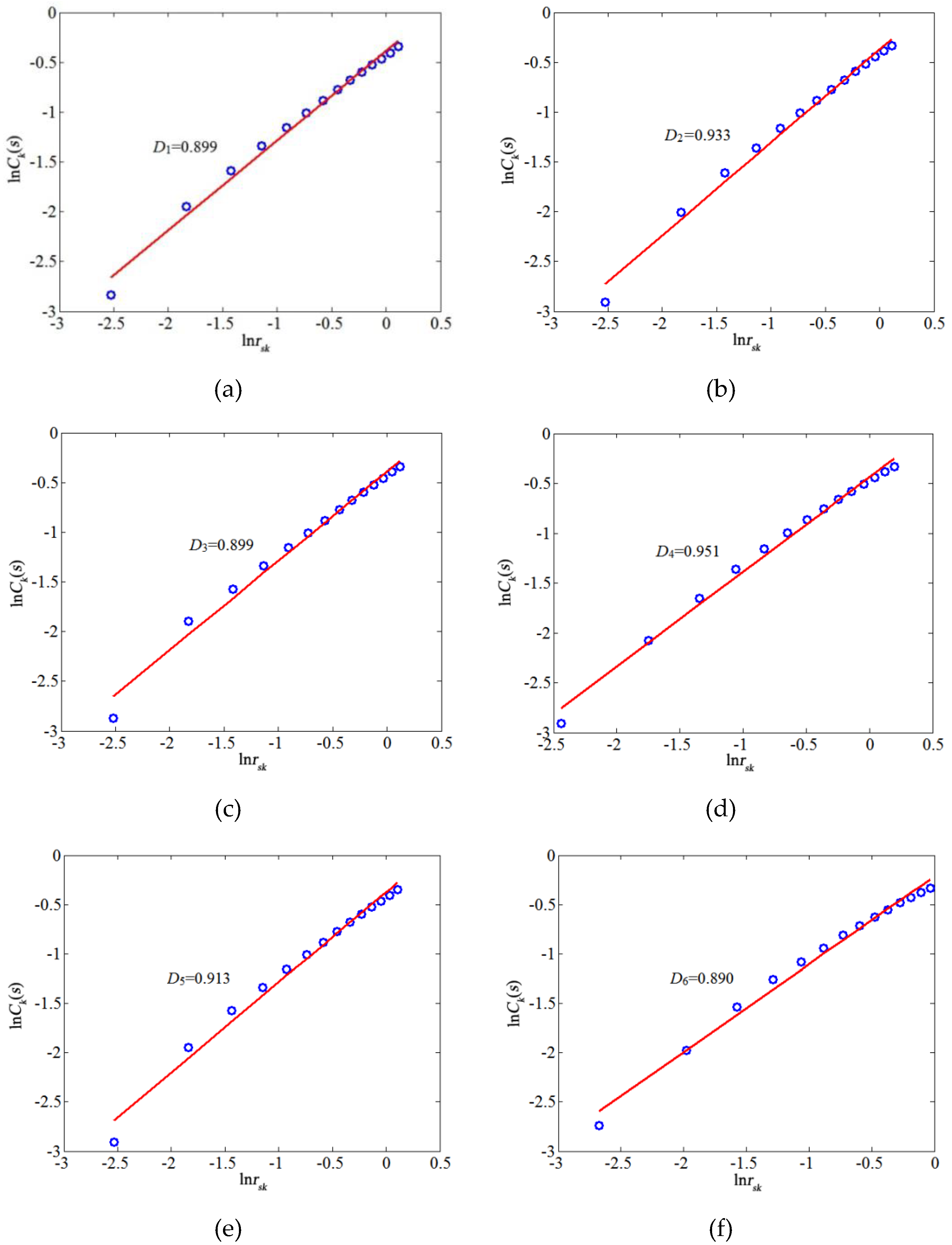
Following the above steps, the fractal dimensions of the six indices in nine-dimensional phase space were calculated as D = (0.899, 0.933, 0.899, 0.951, 0.913, 0.890). Figure 6 shows the fitting curves of lnC_k(s) and lnr_sk, and the slope is the fractal dimension.

Roughly speaking, the fractal dimension is the slope of the fitting line obtained by fitting a set of points (lnC_k(s), lnr_sk). This calculation is easy to achieve through a MATLAB program. The bigger the fractal dimension of the index is, more important the index is.

(7) Diagnosis function of seismic vulnerability. Combining the fractal dimension vector D, the comprehensive assessment value vector Z was obtained in light of Formula (10), according to

Table 6. Comparison table for evaluation results.

No.	The Proposed Method in This Paper			AHP-Based Assessment Method [27]		Catastrophe Progression Method [26,52]
	Evaluation Value	Grade Value	Grade	Evaluation value	Grade	Evaluation value	Grade
1	2.697	2	II	0.468	II	0.895	II
2	2.913	2.2	[II,III]	0.568	III	0.915	III
3	2.853	2	II	0.551	III	0.915	III
4	2.853	2	II	0.491	II	0.900	II
5	2.882	2.0	II	0.486	II	0.900	II
6	2.229	2	II	0.472	II	0.842	II
7	2.562	2	II	0.440	II	0.883	II
8	3.002	2.7	[II,III]	0.572	III	0.919	III
9	2.630	2	II	0.524	III	0.906	II
10	2.386	2	II	0.480	II	0.850	II
11	2.852	2	II	0.550	III	0.915	III
12	2.318	2	II	0.476	II	0.845	II
13	2.698	2	II	0.528	III	0.909	II
14	2.453	2	II	0.484	II	0.854	II
15	2.696	2	II	0.527	III	0.909	II
16	3.381	3	III	0.665	III	0.930	III
17	2.562	2	II	0.440	II	0.883	II
18	3.701	3	III	0.711	III	0.945	III
19	2.882	2.0	II	0.486	II	0.900	II

.

$$Z(j)={\displaystyle \sum _{i=1}^m{D}_i}\times x_{ij}$$

(10)

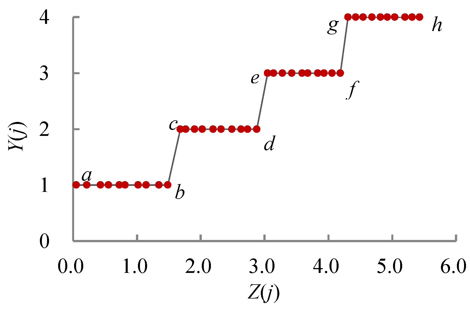
Figure 7 shows a step curve. The comprehensive assessment value Z(j) in segments a–b, c–d, e–f, and g–h corresponds to the vulnerability grade Y(j) = 1, 2, 3, 4, respectively. The grade eigenvalue in segments b–c, d–e, and f–g can be obtained through linear interpolation of Z(j). Therefore, the diagnosis function Y(j) of the seismic vulnerability grade and the synthetic appraisal value of the jth sample are expressed respectively as follows:

$$Y\left(j\right)=\{\begin{array}{l}1,Z\left(j\right)\le 1.484\\ 1+\frac{Z\left(j\right)-1.484}{1.681-1.484},1.484<Z\left(j\right)<1.681\\ 2,1.681\le Z\left(j\right)\le 2.880\\ 2+\frac{Z\left(j\right)-2.880}{3.048-2.880},2.880<Z\left(j\right)<3.048\\ 3,3.048\le Z\left(j\right)\le 4.187\\ 3+\frac{Z\left(j\right)-4.187}{4.308-4.187},4.187<Z\left(j\right)<4.308\\ 4,4.308\le Z\left(j\right)\end{array}$$

(11)

$$Z(j)=0.899\times x_{1j}+0.993\times x_{2j}+0.899\times x_{3j}+0.951\times x_{4j}+0.913\times x_{5j}+0.890\times x_{6j}$$

(12)

3. Case Study

3.1. Feasibility Analysis of the Model

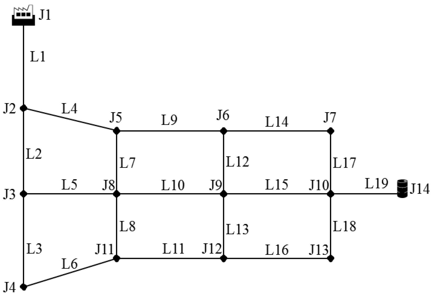
To verify the feasibility of the model, it was applied in a WSN of a city in South China. A WSN in some area of the city was chosen as a calculation case, which facilitated the following analysis and the comparison of results. There were 19 pipelines (i.e., L1–L19) and 14 nodes (i.e., J1–J14) in the WSN, as shown in Figure 8. Node J1 was the water plant, and node J14 was the water tower. The basic data of pipelines are shown in

Table 7. Basic data of the water supply pipelines.

No	x1	x2 /mm	x3	x4 /Years	x5	x6 /m
1	Concrete pipe	800	Rubber ring	20	3	1.1
2	Steel pipe	400	Welding	13	3	1.1
3	Steel pipe	600	Welding	20	3	1.1
4	Concrete pipe	600	Rubber ring	20	3	1.1
5	Grey cast-iron pipe	300	Rubber ring	15	3	0.7
6	Steel pipe	1200	Welding	10	3	1.2
7	Nodular cast iron pipe	300	Rubber ring	8	3	0.7
8	Steel pipe	400	Welding	13	3	0.7
9	Steel pipe	800	Welding	15	3	1.1
10	Steel pipe	1200	Welding	15	3	0.8
11	Steel pipe	600	Welding	15	3	0.8
12	Steel pipe	1200	Welding	10	3	0.8
13	Steel pipe	800	Welding	20	3	1.1
14	Steel pipe	1200	Welding	20	3	0.8
15	Steel pipe	800	Welding	15	3	0.8
16	Nodular cast-iron pipe	200	Asbestos cement	8	3	0.4
17	Nodular cast-iron pipe	300	Rubber ring	8	3	0.7
18	Gray cast-iron pipe	200	Asbestos cement	15	3	0.4
19	Gray cast-iron pipe	300	Rubber ring	15	3	0.7

.

According to Formulas (1) and (2), the index data in Table 7 were standardized, and the comprehensive assessment values of the 19 samples were calculated based on Formula (12). Finally, we obtained the vulnerability grades of water supply pipelines against earthquake disasters, and comparative analysis with other methods was performed. The results are shown in Table 6.

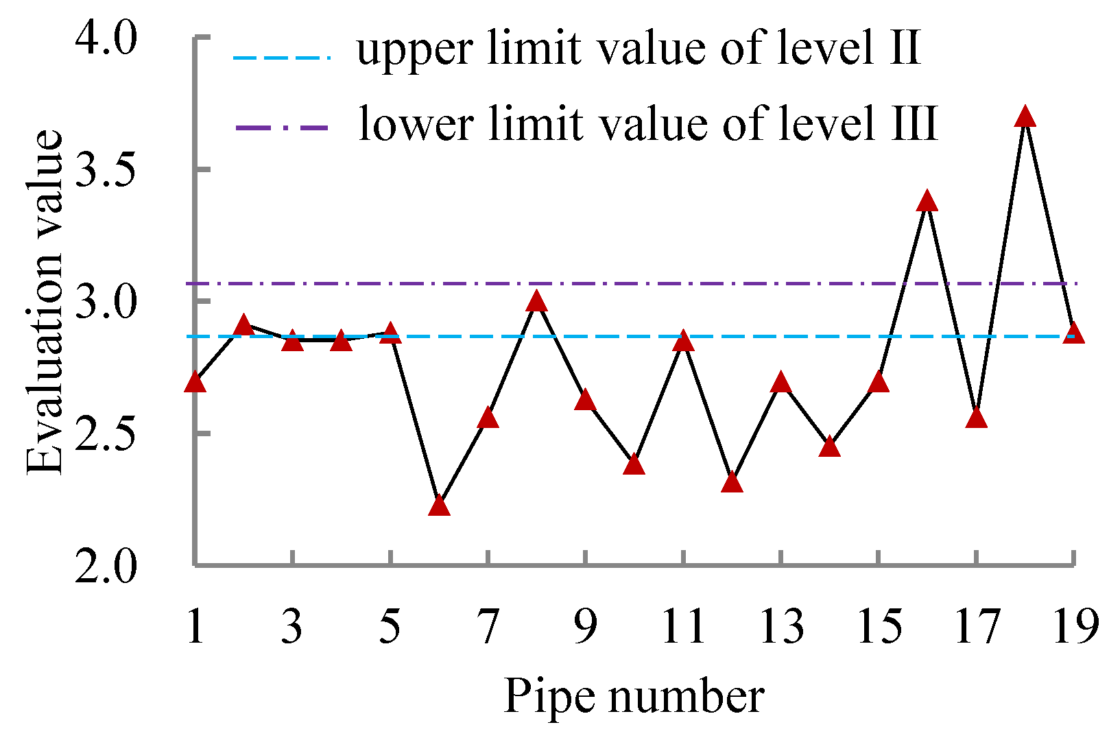
Table 6 showed that Pipes 8, 16, and 18 were at moderate vulnerability (i.e., Grade III), and the others were at low vulnerability (i.e., Grade II). In addition, the vulnerability order of the pipes was obtained according to the evaluation values. The evaluation results obtained by the proposed method basically agree with the results of the catastrophe progression method, but the result of the proposed method was subtly different from that of the analytic hierarchy process (AHP)-based method. The reason was that determination of the index weight had influence on the final assessment, and the nonlinear relation between indices was not considered by the AHP-based method. Though the catastrophe progression method considered the nonlinear relationship between indices, it needed to determine the order of index weights, and there were still some subjective influences. The weights of fractal dimension were calculated using the index data and the nonlinear relationships among indices were taken into account in the method proposed in this paper. Therefore, the evaluation results obtained by the method proposed in this paper were more reasonable and objective.

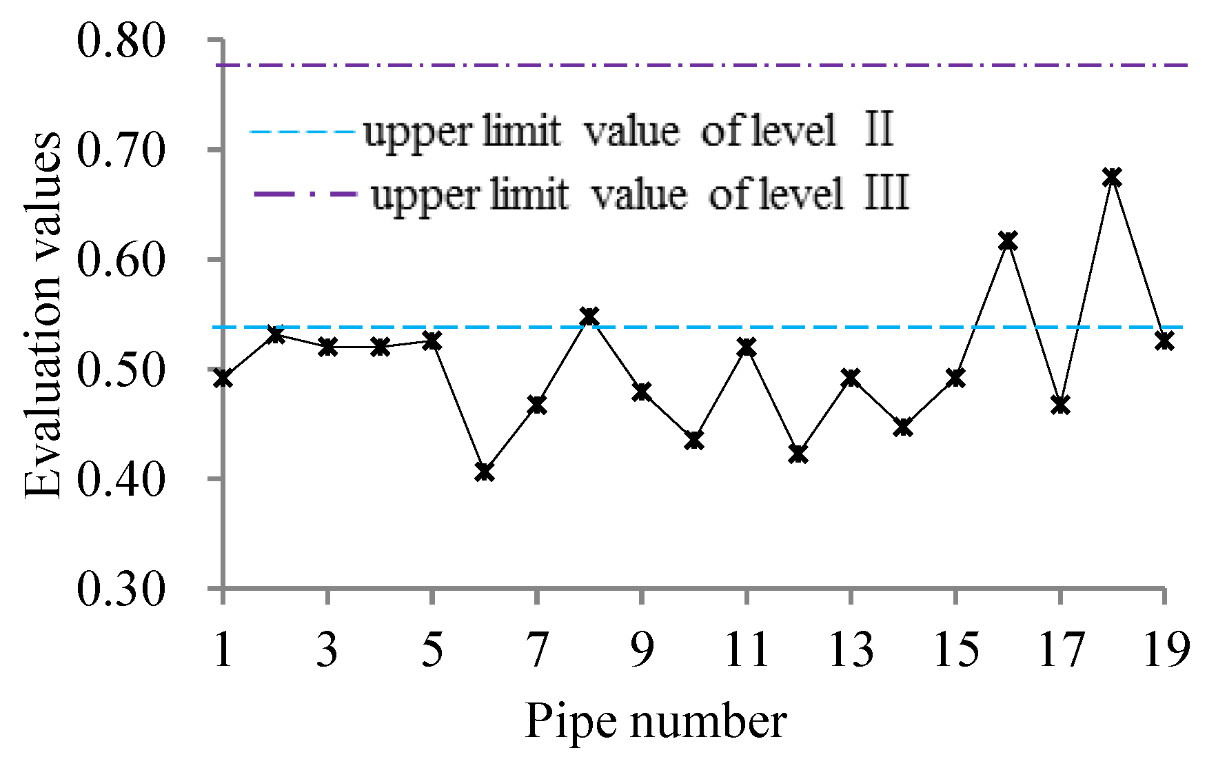
Figure 9 shows the scatter diagram of the evaluation results of the proposed method. For comparison with the other two methods, the weight coefficient was obtained by normalizing fractal dimension, and then the evaluation results that were obtained are shown in Figure 10.

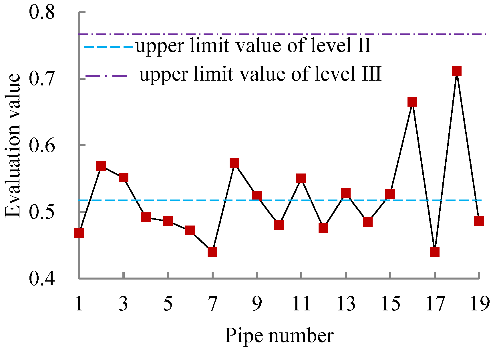
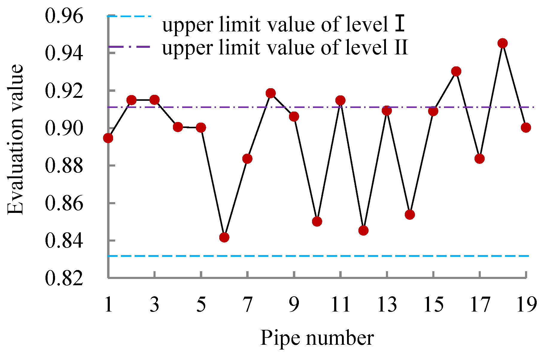
Figure 10, Figure 11 and Figure 12 showed the scatter diagram of evaluation results obtained by the three methods, respectively. The variation tendencies of the scatter curves in Figure 10, Figure 11 and Figure 12 were largely consistent. In particular, they were completely consistent in Figure 10 and Figure 12, which indicated that the two methods could accurately describe the vulnerability state of the pipeline in the entire water supply network. However, there was a fuzzy interval between the upper limit values of levelIIand the lower limit value of level III in Figure 9. In the fuzzy interval, the vulnerability grade was judged based on the minimal distance principle in this paper, which was successful in dealing with the fuzzy problems existing in grade boundaries. However, in Figure 11 and Figure 12, the grade boundary was an exact value. They did not consider the fuzzy problems existing in the grade boundaries, which could lead to misinterpretation.

3.2. Application Example

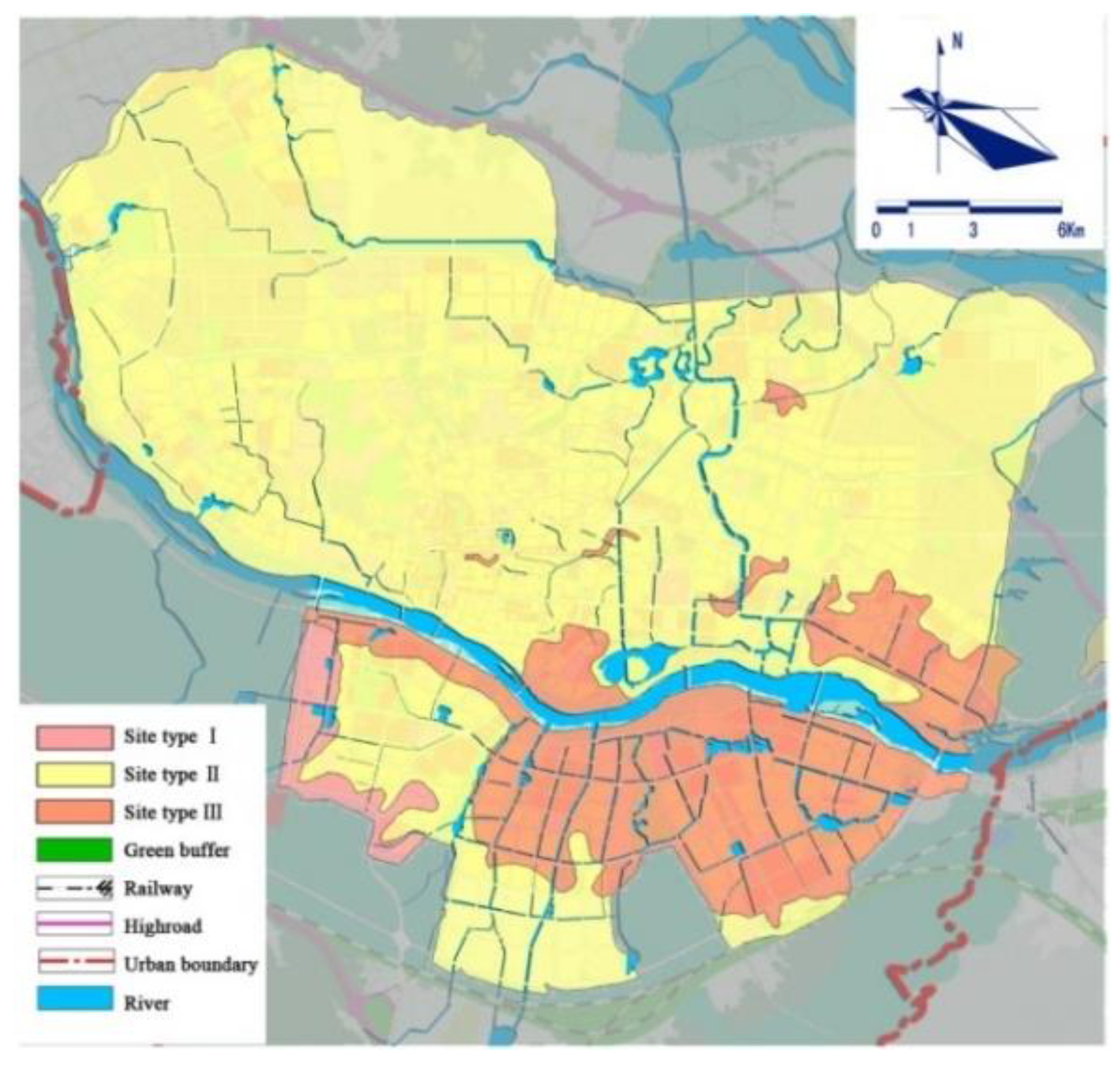
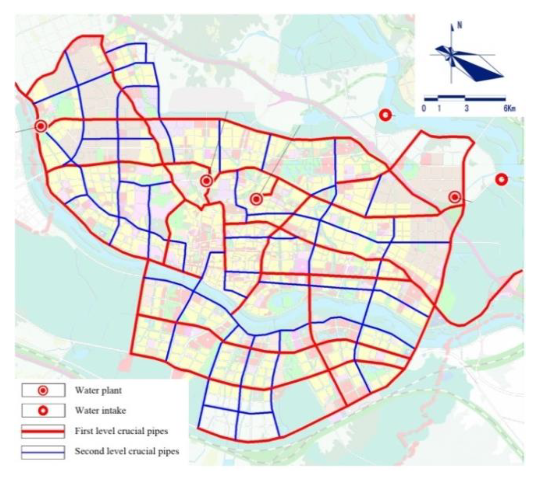
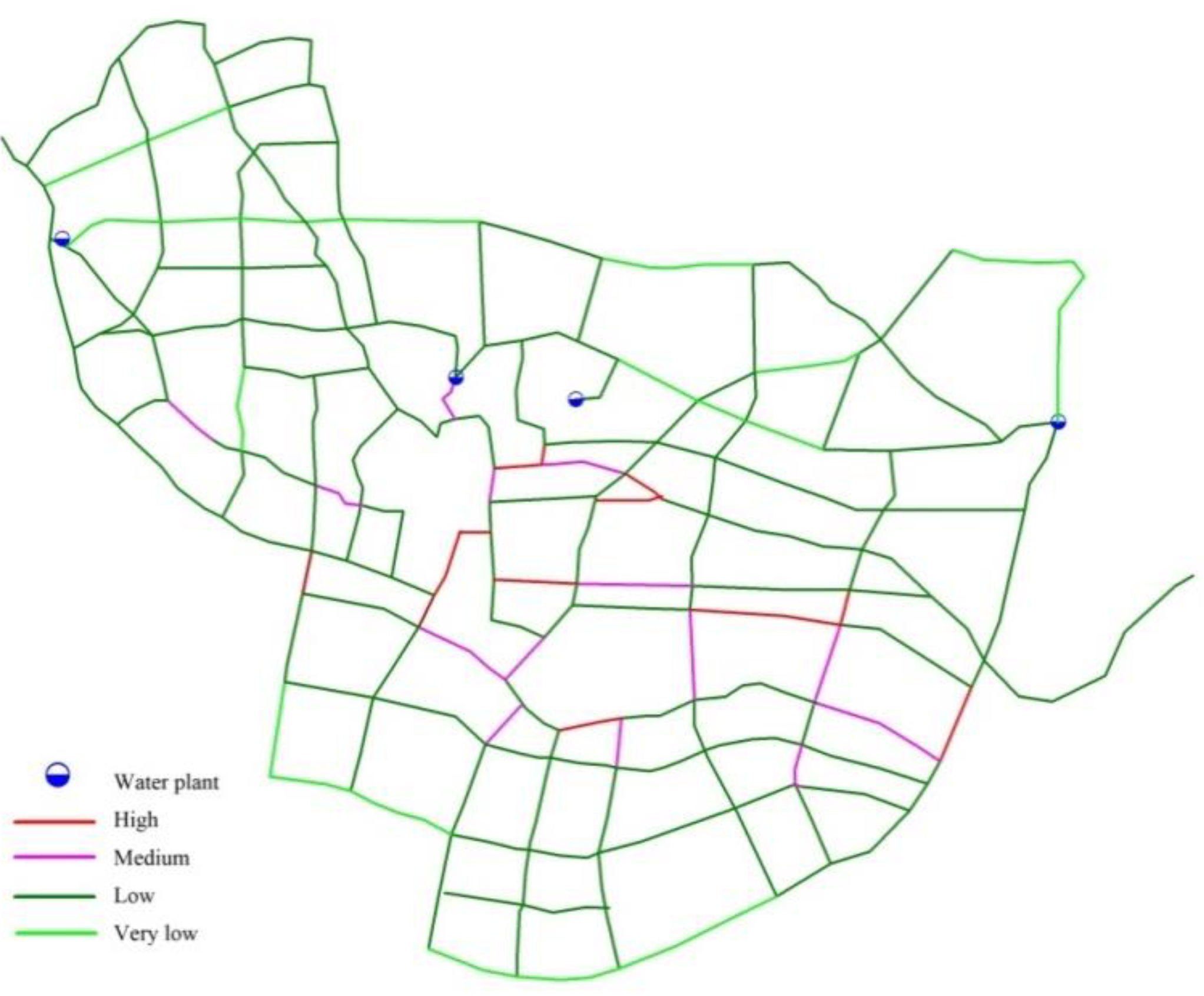
To evaluate the vulnerability of the WSN against earthquake hazards, the model was applied in the WSN of the city. The pipe material, pipe diameter, pipe connection, buried depth, and site type of each pipeline can be obtained by the geographical information management system (GIMS) of the WSN. Figure 13 shows the distribution of site types in the whole city. Figure 14 shows the distribution of crucial pipelines for disaster prevention in the city.

Based on the above-mentioned information, the seismic vulnerability level of the WSN can be evaluated by Formulas (11) and (12). The final evaluation results were visually represented in the GIMS of the WSN, as shown in Figure 15. They showed that the pipelines with high vulnerability were mainly distributed in the older area of the city. They were mainly plain cast-iron pipes of less than 300 mm in diameter and more than 50 years older in pipe age, pre-stressed concrete pipes more than 30 years older, and partly steel pipes more than 20 years older. Therefore, we need to develop a renovation planning of the water supply network and a regular troubleshooting scheme. When renovating pipe networks or laying new pipes, the following disaster prevention requirements must be followed: 1) First, improve the pipelines with high vulnerability and the older ones. Choose a pipeline with good seismic performance and flexible joints; 2) formulate a plan to phase out gray cast-iron pipes, galvanized steel pipes, self-stressing concrete tube, plain cast-iron pipes with small diameters, and so on; 3) regularly monitor the operation status of pipelines in special zones (cross-river or soft and liquefiable ground, for instance), and dispose of the risks in time.

4. Conclusions

Earthquake vulnerability evaluation of WSNs is a complex nonlinear system problem. A fractal interpolation function model for seismic vulnerability grade recognition of water supply pipelines was established based on fractal theory, which had great superiority in solving nonlinear problems. Firstly, the main impact factors on seismic vulnerability were chosen on the basis of the concept and formation mechanism of vulnerability. Grading standards for seismic vulnerability of pipelines were initially established. On the basis of the grading standards, a vulnerability grade function was given based on random interpolation and fractal dimension.

The model was used to assess the seismic vulnerability grade of a WSN to verify its feasibility. The results showed that: 1) Pipes 8, 16, and 18 were at a medium vulnerability level (i.e., Grade III). Other pipelines were at a low vulnerability level (i.e., Grade II). 2) The whole network was in good working condition. 3) We could obtain the seismic vulnerability grades as well as the assessment values of pipelines using the model, and we could sort the samples at the same vulnerability level. 4) Through comparative analysis, the results obtained by the model were generally consistent with those obtained by the catastrophe progression method. The shape of the scatter plots of the assessment values respectively obtained by the three methods is similar to some extent. However, the model proposed in this study took the fuzziness of grading limit into account, and its feasibility and reliability were verified by the comparative analysis.

The model was finally applied to a WSN in South China. This indicated that the pipelines with high vulnerability were mainly distributed in the older areas of the city. Aiming at this case, this paper proposed the development of a renovation planning of the WSN and gave some disaster prevention requirements.

References

- Kanta, L.; Brumbelow, K. Vulnerability, risk, and mitigation assessment of water distribution system for insufficient fire flows. J. Water Resour. Plann Manag. 2013, 139, 593–603. [Google Scholar] [CrossRef]
- Laucelli, D.; Giustolisi, O. Vulnerability assessment of water distribution networks under seismic actions. J. Water Resour. Plann Manage. 2015, 141, 04014082-1–04014082-14. [Google Scholar] [CrossRef]
- Yang, S.L.; Hsu, N.S.; Loule, P.W.F.; Yeh, W.W.G. Water distribution network reliability: Connectivity analysis. J. Infrastruct. Syst. 1996, 2, 54–64. [Google Scholar] [CrossRef]
- Yazdani, A.; Otoo, R.A.; Jeffrey, P. Resilience enhancing expansion strategies for water distribution systems: A network theory approach. Environ. Model Softw. 2011, 26, 1574–1582. [Google Scholar] [CrossRef]
- Wang, S.W.; Wang, Y.; Qian, Z.H.; Liu, S.Q.; Yuan, W.Q.; Zheng, X.M. Investigation and analysis about damage and recovery of water supply system in 5.12 earthquake areas. China Water Wastewater 2009, 25, 2–11. [Google Scholar]
- Miyajima, M. Damage analysis of water supply facilities in the 2011 great east Japan earthquake and tsunami. In Proceedings of the 15th World Conference in Earthquake Engineering, Lisbon, Portugal, 28 September 2012; pp. 24–25. [Google Scholar]
- Giovinazzi, S.; Wilson, T.M.; Davis, C. Lifelines Performance and Management Following the 22 February 2011 Christchurch Earthquake; Highlights of resilience, University of Canterbury: Canterbury, New Zealand, 2011. [Google Scholar]
- Scawthorn, C.; Yamada, Y.; Iemura, H. A model for urban post-earthquake fire hazard. Disasters 1981, 5, 125–132. [Google Scholar] [CrossRef]
- Coppola, D. Introduction to Disaster Management; Elsevier: San Diego, CA, USA, 2007. [Google Scholar]
- Zhou, J.H. Destructive Test Study and Aseismic Analysis of Water Supply Pipeline. Doctoral Dissertation, University of Technology, Dalian, China, 2010. [Google Scholar]
- Toprak, S.; Taskin, F. Estimation of earthquake damage to buried pipelines caused by ground shaking. Nat. Hazards 2007, 40, 1–24. [Google Scholar] [CrossRef]
- Wang, Y.H.; Li, S.C.; Zhong, X.B.; Tian, B.P. Seismic reliability analysis of urban water supply system. World Earthq. Eng. 2014, 30, 224–228. [Google Scholar]
- He, S.H.; Zhao, Y.; Song, C. Seismic connectivity reliability analysis of urban water supply network. J. Disaster Prev. Mitig. Eng. 2011, 31, 585–589. [Google Scholar]
- Liu, W.; Zhao, Y.G.; Li, J. Seismic functional reliability analysis of water distribution networks. Struct. Infrastruct. Eng. 2015, 11, 363–375. [Google Scholar] [CrossRef]
- Hou, B.W.; Du, X.L.; Wang, W. Seismic performance based design of water distribution system considering comprehensive importance of users. China Civil Eng. J. 2015, 48, 11–22. [Google Scholar]
- Liu, W.; Xu, L.; Li, J. Algorithms for seismic topology optimization of water distribution network. Sci. China Technol. Sci. 2012, 55, 3047–3056. [Google Scholar] [CrossRef]
- Cimellaro, G.P.; Solari, D.; Bruneau, M. Physical infrastructure interdependency and regional resilience index after the 2011 Tohoku earthquake in Japan. Earthq. Eng. Struct. Dyn. 2014, 43, 1763–1784. [Google Scholar] [CrossRef]
- Luna, R.; Balakrishnan, N.; Dagli, C.H. Post-earthquake recovery of a water distribution system: Discrete event simulation using colored petri nets. J. Infrastruct. Syst. 2011, 17, 25–34. [Google Scholar] [CrossRef]
- Kozin, F.; Zhou, H. System study of urban response and reconstruction due to earthquake. J. Eng. Mech. 1990, 116, 1959–1972. [Google Scholar] [CrossRef]
- Tabucchi, T.; Davidson, R.; Brink, S. Simulation of post-earthquake water supply system restoration. Civil Eng. Environ. Syst. 2010, 27, 263–279. [Google Scholar] [CrossRef]
- Turner, J.P.; Qiao, J.; Lawley, M.; Richard, J.; Abraham, D.M. Mitigating shortage and distribution costs in damaged water networks. Socio-Econ. Plan. Sci. 2012, 46, 315–326. [Google Scholar] [CrossRef]
- Yoo, D.G.; Jung, D.; Kang, D.; Kim, J.H.; Lansey, K. Seismic hazard assessment model for urban water supply networks. J. Water Resour. Plann. Manag. 2016, 142, 04015055. [Google Scholar] [CrossRef]
- Christodoulou, S.E.; Fragiadakis, M. Vulnerability assessment of water distribution networks considering performance data. J. Infrastruct. Syst. 2015. [Google Scholar] [CrossRef]
- Zhang, Z.P.; Wang, Z.T.; Su, J.Y.; Wang, W. Research on the seismic damage assessment of underground pipelines. China Rural Water Hydropower 2013, 8, 43–47. [Google Scholar]
- Bai, J.L. Study on the seismic risk control of water supply pipelines. Tianjin University: Tianjin, China, 2011. [Google Scholar]
- Wu, J.; Liu, W.L.; Liang, J.; Feng, B.R. Seismic vulnerability evaluation of Beijing’s water supply pipeline. J. Wuhan Univ. Technol. (Inf. Manag. Eng.) 2017, 39, 140–143. [Google Scholar]
- Wang, Z.T.; Wang, W.; Guo, X.D. Seismic vulnerability assessment for water supply network based on nodes importance. Disaster Adv. 2013, 6, 430–436. [Google Scholar]
- Halfaya, F.Z.; Bensaibi, M.; Davenne, L. Seismic vulnerability of buried water pipes. Adv. Environ. Sci. Eng. 2012. [Google Scholar] [CrossRef]
- O’Rourke, M.J.; Ayala, G. Pipeline damage due to wave propagation. J. Geotech. Eng. 1993, 119, 123–134. [Google Scholar] [CrossRef]
- Burton, I.; Katers, R.W.; White, G.F. The Environment as Hazard, 2nd ed.; The Guildford Press: New York, NY, USA, 1993. [Google Scholar]
- Shi, P.J. Theory and practice of disaster study. J. Nat. Disaster 1996, 5, 6–17. [Google Scholar]
- Wisner, B.; Blaikie, P.; Cannon, T.; Davis, I. At Risk: Natural Hazards, People’s Vulnerability and Disasters, 2nd ed.; Routledge: London, UK, 2004. [Google Scholar]
- United Nations Disaster Relief Organization. Mitigating Natural Disasters Phenomenal Effects and Options a Manual for Policy Makers and Planners; United Nations Disaster Relief Organization: New York, NY, USA, 1991. [Google Scholar]
- Gentile, F.; Bisantino, T.; Trisorio, L.G. Debris-flow risk analysis in south Gargano watersheds (Southern Italy). Nat. Hazards 2008, 44, 1–17. [Google Scholar] [CrossRef]
- United States Agency for International Development. Interduction to Disaster Risk Reduction; USAI: Washington, DC, USA, 2011.
- McGuire, B.; Mason, I.; Kiburn, C. Natural Hazards and Environmental Change; Arnold: London, UK, 2002. [Google Scholar]
- Intentional Strategy for Disaster Reduction. Living with Risk, A Global Review of Disaster Reduction Initiatives; United Nations publication: Geneva, Switzerland, 2004. [Google Scholar]
- Alexander, D. Natural Disaster; UCL Press: London, UK, 1993. [Google Scholar]
- Smith, K. Environmental Hazards: Assessing Risk and Reducing Disaster, 3rd ed.; Routledge: New York, NY, USA, 2000. [Google Scholar]
- Gill, J.C.; Malamud, B.D. Reviewing and visualizing the interaction of natural hazards. Rev. Geophys. 2014, 52, 680–722. [Google Scholar] [CrossRef] [Green Version]
- Jin, S.M. Research on Earthquake Disaster Risk and Resilience of Urban Water Supply System. Master Dissertation, Institute of Technology, Harbin, China, 2013. [Google Scholar]
- Balica, S.F.; Douben, N.; Wright, N.G. Flood vulnerability indices at varying spatial scales. Water Sci. Technol. 2009, 60, 2571–2580. [Google Scholar] [CrossRef]
- United Nations International Strategy for Disaster Reduction. UNISDR Terminology for Disaster Risk Reduction; United Nations International Strategy for Disaster Reduction (UNISDR): Geneva, Switzerland, 2009. [Google Scholar]
- Balica, S.F.; Wright, N.G.; Meulen, F. A flood vulnerability index for coastal cities and its use in assessing climate change impacts. Nat. Hazards 2012, 64, 73–105. [Google Scholar] [CrossRef] [Green Version]
- Ndah, A.B.; Odihi, J.O. A systematic study of disaster risk in Brunei Darussalam and options for vulnerability-based disaster risk reduction. Int. J. Disaster Risk Sci. 2017, 8, 208–223. [Google Scholar] [CrossRef] [Green Version]
- Ye, Y.X.; Okada, N. Earthquake Disaster Comparatology; China Building Industry Press: Beijing, China, 2008. [Google Scholar]
- Yang, C. Study on Seismic Damage Assessment of Urban Water Supply Pipe Network. Master’s Thesis, Zhejiang University, Hangzhou, China, 2010. [Google Scholar]
- Liu, H.X. Earthquake Damage of Tangshan Earth- Quake; Seismological Press: Beijing, China, 1986. [Google Scholar]
- Jiang, H. Analysis of Buried Pipeline Response to Seismic Wave Propagation. Master’s Thesis, Huazhong University of Science & Technology, Wuhan, China, 2011. [Google Scholar]
- Wu, G.Z.; Xu, Z.X.; Li, C.Y. Water eutrophication assessment and validation based on fractal theory. Water Resour. Prot. 2012, 28, 12–16. [Google Scholar]
- Niu, Y.C.; Zhou, Z.F.; Wang, L.; Dan, Y.S.; Feng, Q. Comprehensive evaluation of soil nutrients in Guizhou agricultural products areas based on the fractal interpolation model. Environ. Chem. 2018, 37, 2207–2218. [Google Scholar]
- Nu, Z.G.; Jiang, W.; Lu, R.Q.; Zhang, H.W. Research on the vulnerability assessment model of water supply systems based on catastrophe theory. J. Harbin Inst. Technol. 2012, 44, 135–138. [Google Scholar]
Figure 1.
The algorithm diagram of the theoretical framework.
Figure 2.
Damage rates of different pipes in the Kobe earthquake.
Figure 3.
The relationship between pipe diameter and damage rate of Ashiya in the Kobe earthquake.
Figure 4.
The relationship between pipe diameter and damage rate in the Tangshan earthquake.
Figure 5.
The relationship between pipe diameter and damage rate of cast-iron pipes with asbestos cement joints in Yingkou city after the Haicheng earthquake.
Figure 6.
Fitted curves of lnCk(s)—lnrsk: (a) Pipe material, (b) pipe diameter, (c) joint type, (d) pipe age, (e) site classification, and (f) buried depth.
Figure 7.
Scatter plot graph between Z(j) and Y j).
Figure 8.
Sketches of the water supply network.
Figure 9.
Results obtained by the proposed method.
Figure 10.
Results obtained by the proposed method (fractal dimension normalization).
Figure 11.
Results obtained by the AHP-based method.
Figure 12.
Results obtained by the catastrophe progression method.
Figure 13.
Distribution map of site types.
Figure 14.
Layout map of crucial pipes for disaster prevention.
Figure 15.
Vulnerability assessment map of water supply pipelines.