Temporal and Spatial Variability of Carbon Emission Intensity of Urban Residential Buildings: Testing the Effect of Economics and Geographic Location in China


Abstract
:Highlights
Abstract
1. Introduction
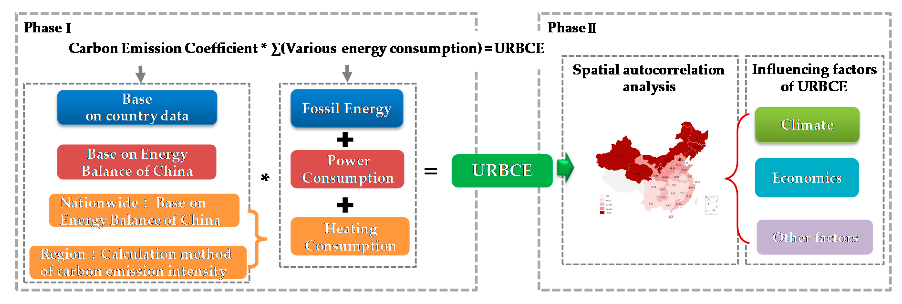
2. Method
2.1. Carbon Emissions and Intensities of URBs
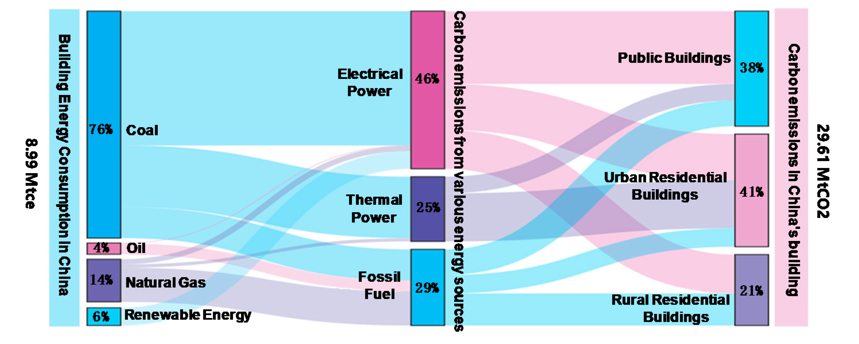
2.1.1. Carbon Emission in URBs
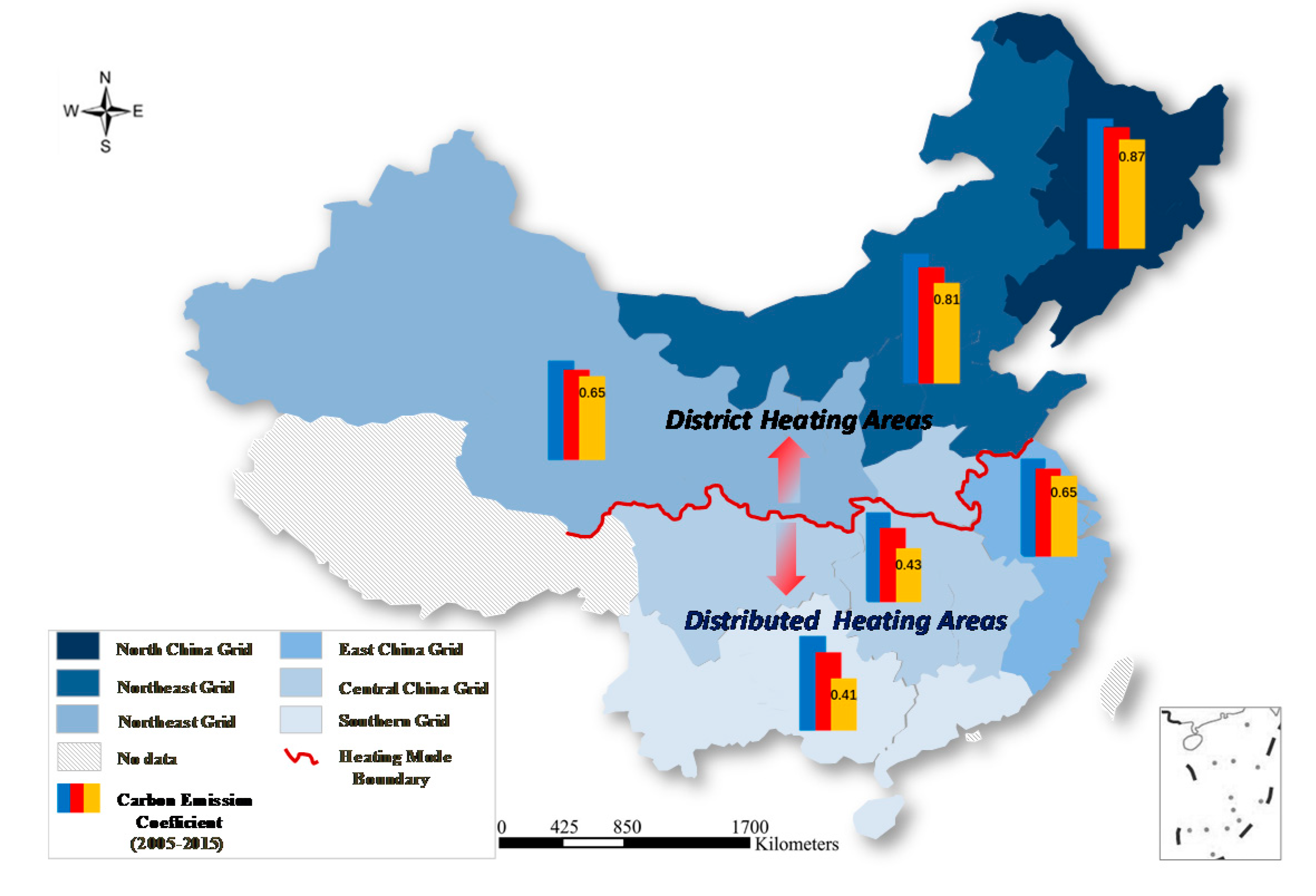
2.1.2. Carbon Emission Coefficient of Electric Power
2.1.3. Thermal Carbon Emission Coefficient
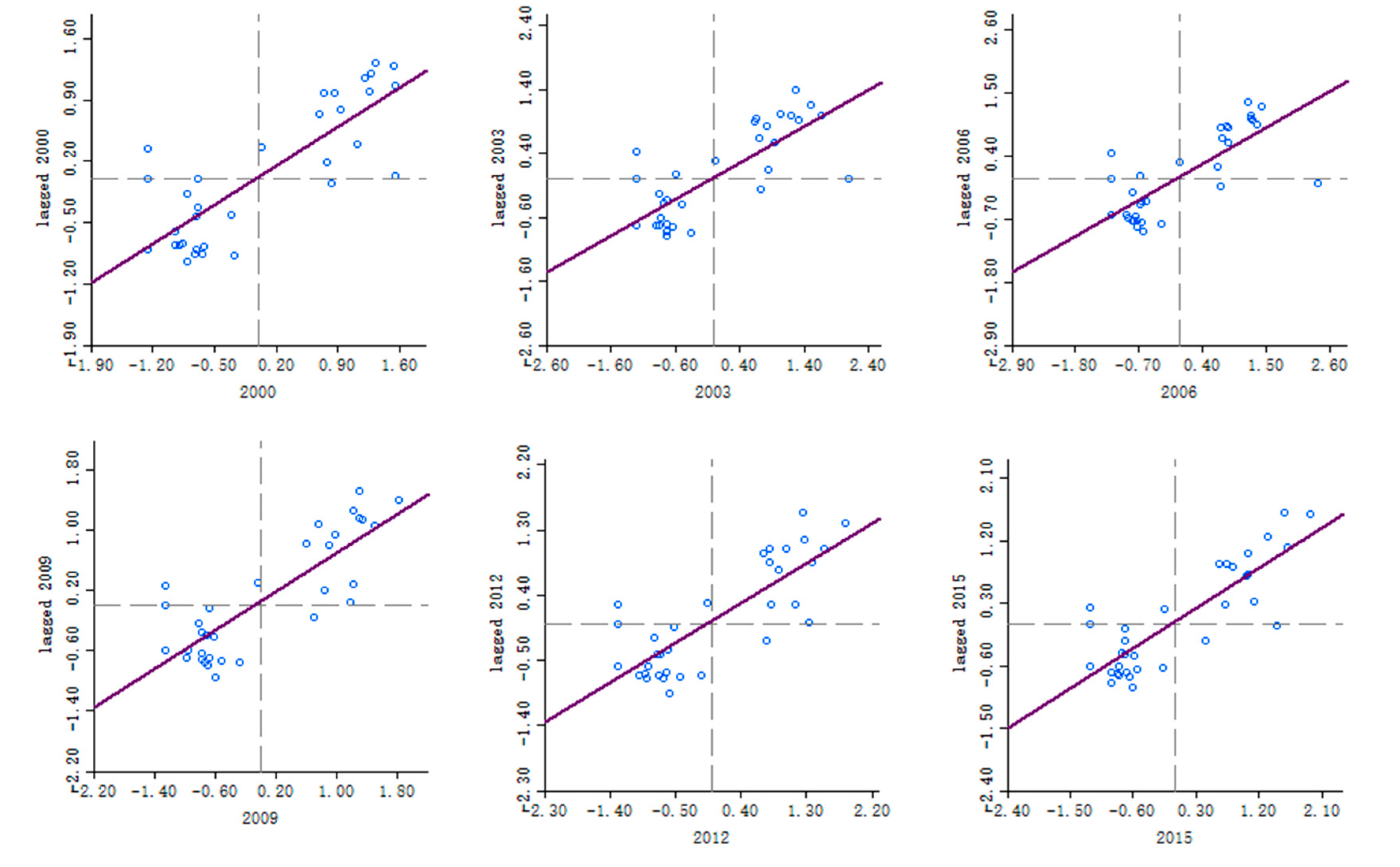
2.2. Spatial Autocorrelation Analysis
2.2.1. Global Spatial Autocorrelation
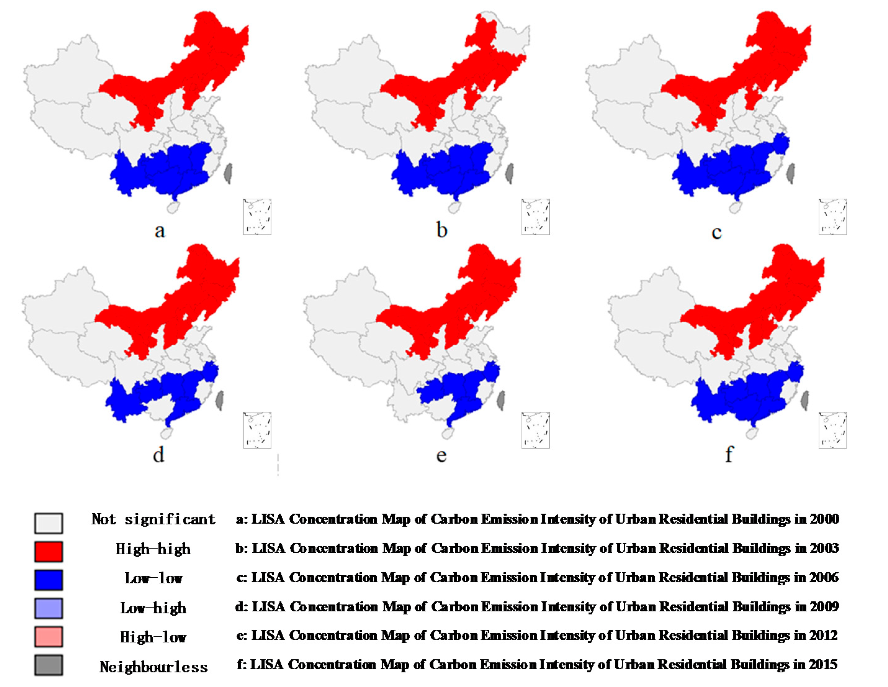
2.2.2. Local Spatial Autocorrelation
2.3. Spatial Panel Measurement Model
3. Variable Selection and Data Source
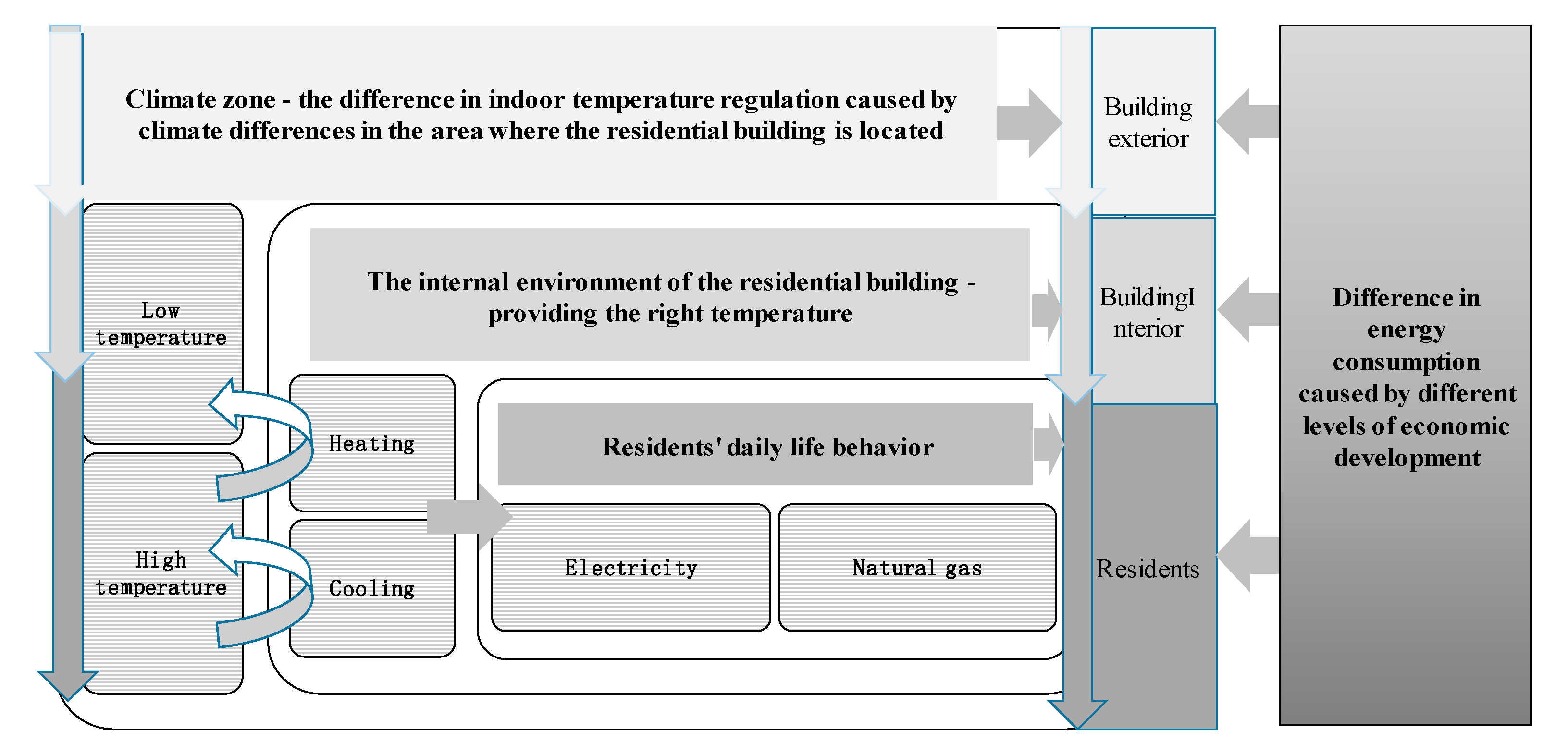
3.1. Variable Selection
3.2. Data Source and Processing
4. Spatiotemporal Evolution of Carbon Emission Intensity
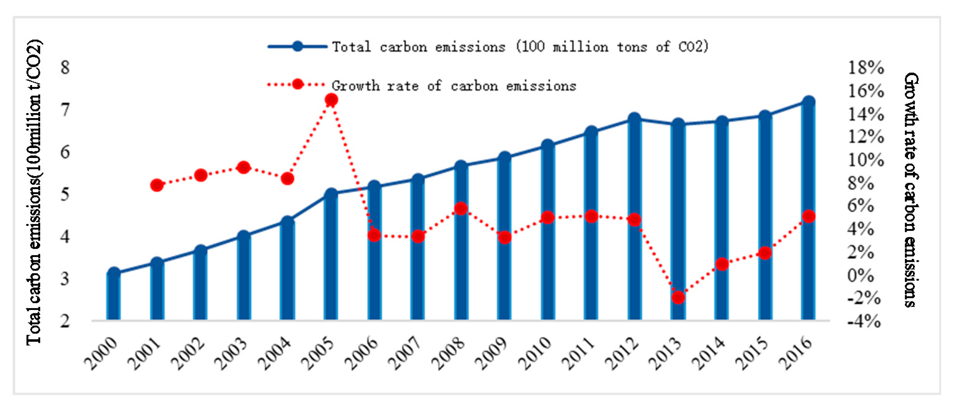
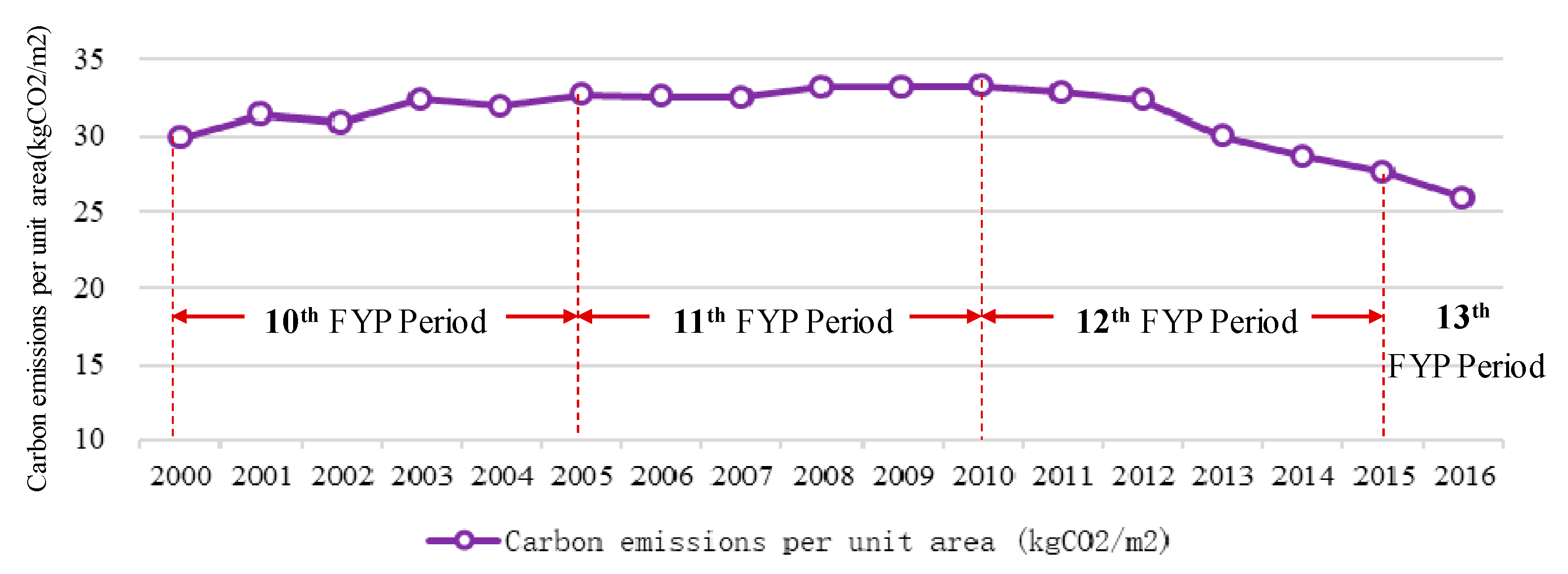
4.1. Temporal Evolution of LC and Its Intensity
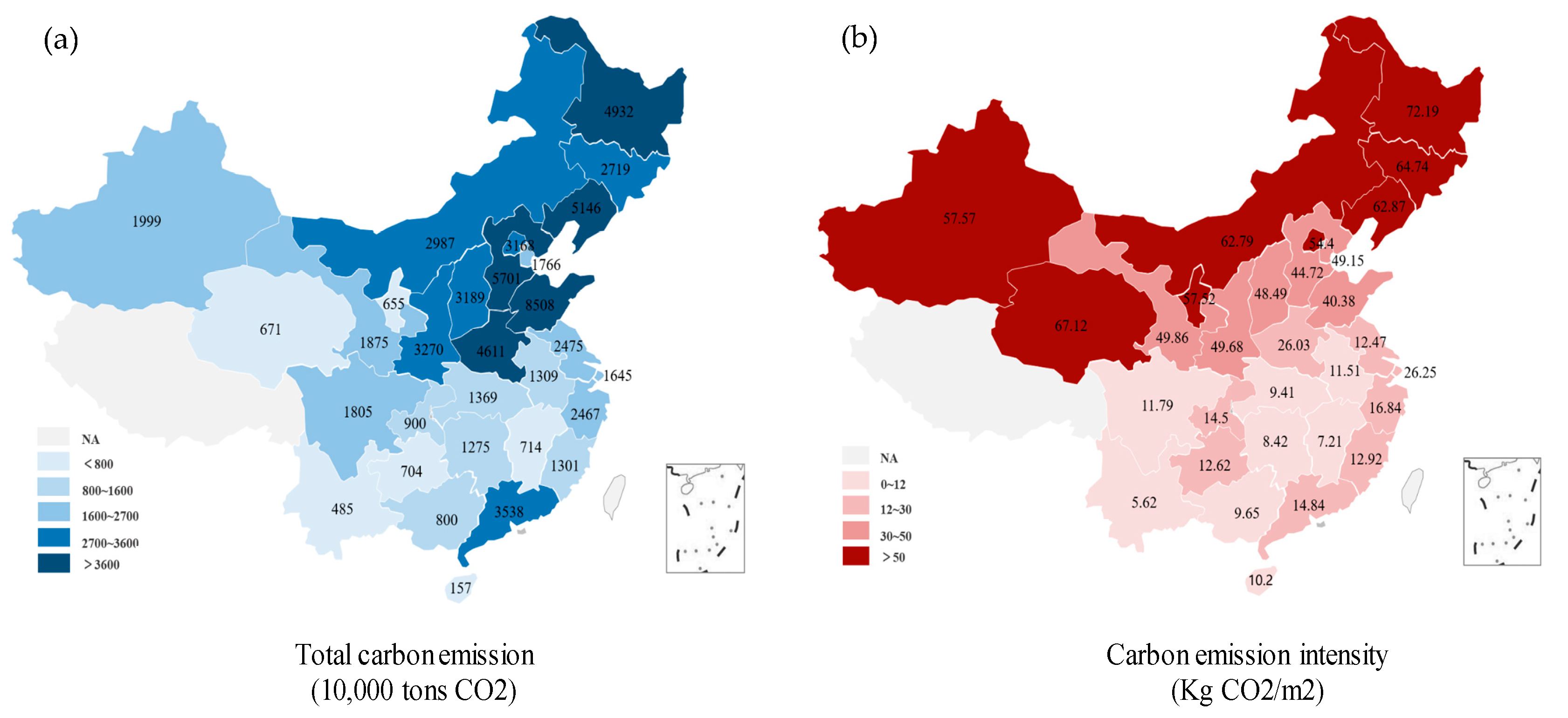
4.2. Regional Carbon Emissions and Intensity of URBs
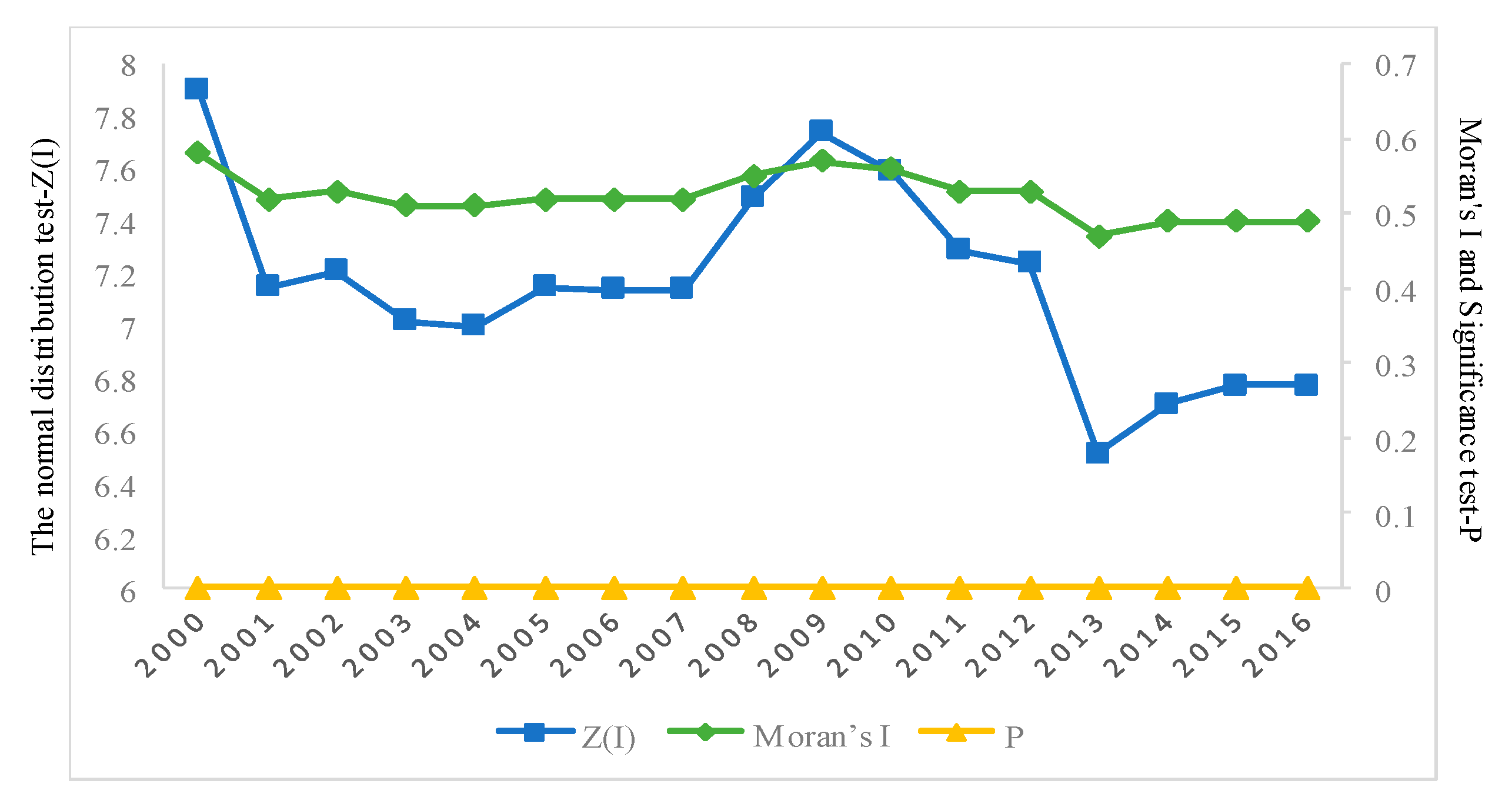
4.3. Spatial Evolution of Carbon Emission and Its Intensity
5. Influencing Factors of URBCE Intensity
6. Conclusions
Author Contributions
Funding
Conflicts of Interest
Nomenclature
| E | Carbon emission of residential buildings |
| C | Energy consumption |
| f | Carbon emission coefficient |
| T | Amount of thermal power generation |
| R | Amount of renewable energy generation |
| EF | Comprehensive carbon emission intensity |
| eei | Energy consumption intensity of heating technical type |
| etij | Proportion of j-th energy consumed by the i-th heating technique |
Abbreviations
| UEBCE | Urban residential buildings Carbon emission |
| HDD | Heating degree days |
| PGDP | The per capita gross domestic product |
| UCL | Urban residents’ consumption level |
| HEA | The household electrical appliances per household |
| LES | Electricity accounts for total energy consumption of households proportion |
| UR | Urbanization rate |
| LA | Urban residential building area |
| PLA | Urban per capita living building area |
| HEA | The household electrical appliances per household |
| LES | Electricity accounts for total energy consumption of households proportion |
| FYP | Five year plan |
| Greek | |
| δ | Spatial autoregressive coefficient |
| μ | Spatial fixed effect |
| λ | Time fixed effect of the model |
| ε | Random error term |
| ρ | Spatial autocorrelation coefficient of the error term |
| ϕ | Spatial error autocorrelation error term |
| Subscripts | |
| Natural gas | |
| Liquefied petroleum gas | |
| Electric power | |
| Thermal energy | |
| Coal | |
| Region | |
| Fossil energy types |
Appendix A

Appendix B

References
- International Energy Agency. World Energy Outlook 2018. IEA 2019. Available online: https://www.iea.org/weo2018/ (accessed on 13 February 2020).
- China Association of Building Energy Efficiency. China Building Energy Consumption Report; Cai, W.G., Ed.; China Association of Building Energy Efficiency: Beijing, China, 2018. (In Chinese) [Google Scholar]
- Ma, M.; Cai, W. What drives the carbon mitigation in Chinese commercial building sector? Evidence from decomposing an extended Kaya identity. Sci. Total. Environ. 2018, 634, 884–899. [Google Scholar] [CrossRef]
- Fan, J.-L.; Liao, H.; Liang, Q.-M.; Tatano, H.; Liu, C.-F.; Wei, Y.-M. Residential carbon emission evolutions in urban–rural divided China: An end-use and behavior analysis. Appl. Energy 2013, 101, 323–332. [Google Scholar] [CrossRef]
- Shi, K.; Chen, Y.; Li, L.; Huang, C. Spatiotemporal variations of urban CO2 emissions in China: A multiscale perspective. Appl. Energy 2018, 211, 218–229. [Google Scholar] [CrossRef]
- Zhang, Y.; Wang, H.; Liang, S.; Xu, M.; Liu, W.; Li, S.; Zhang, R.; Nielsen, C.P.; Bi, J. Temporal and spatial variations in consumption-based carbon dioxide emissions in China. Renew. Sustain. Energy Rev. 2014, 40, 60–68. [Google Scholar] [CrossRef]
- Zhou, N.; McNeil, M.A.; Levine, M. Energy for 500 million homes drivers and outlook for residential energy consumption in China. Lawrence Berkeley National. Laboratory 2009, 26, 83–89. [Google Scholar]
- Lynn, P.; Nina, K.; Zhou, F. Reinventing Fire: Chinadthe Role of Energy Efficiency in China’s Roadmap to 2050; Presqu’ile Giens: Hyeres, France, 2017. [Google Scholar]
- Zhou, N.; Khanna, N.; Feng, W.; Ke, J.; Levine, M. Scenarios of energy efficiency and CO2 emissions reduction potential in the buildings sector in China to year 2050. Nat. Energy 2018, 3, 978–984. [Google Scholar] [CrossRef]
- McNeil, M.A.; Feng, W.; du Can, S.d.l.R.; Khanna, N.Z.; Ke, J.; Zhou, N. Energy efciency outlook in China’s urban buildings sector through 2030. Energy Policy 2016, 97, 532–539. [Google Scholar] [CrossRef] [Green Version]
- Nie, H.; Kemp, R. Index decomposition analysis of residential energy consumption in China: 2002–2010. Appl. Energy 2014, 121, 10–19. [Google Scholar] [CrossRef]
- Jing, R.; Wang, M.; Wang, W.; Brandon, N.; Li, N.; Chen, J.; Zhao, Y. Economic and environmental multi-optimal design and dispatch of solid oxide fuel cell based CCHP system. Energy Convers. Manag. 2017, 154, 365–379. [Google Scholar] [CrossRef]
- Jing, R.; Zhu, X.; Zhu, Z.; Wang, W.; Meng, C.; Shah, N.; Li, N.; Zhao, Y. A multi-objective optimization and multi-criteria evaluation integrated framework for distributed energy system optimal planning. Energy Convers. Manag. 2018, 166, 445–462. [Google Scholar] [CrossRef]
- Wu, W.; Skye, H. Net-zero Nation: HVAC and PV Systems for Residential Net-Zero Energy Buildings across the United States. Energy Convers. Manag. 2018, 177, 605–628. [Google Scholar] [CrossRef]
- Liang, Y.; Cai, W.; Ma, M. Carbon dioxide intensity and income level in the Chinese megacities’ residential building sector: Decomposition and decoupling analyses. Sci. Total. Environ. 2019, 677, 315–327. [Google Scholar] [CrossRef] [PubMed]
- Zhang, M.; Song, Y.; Li, P.; Li, H. Study on affecting factors of residential energy consumption in urban and rural Jiangsu. Renew. Sustain. Energy Rev. 2016, 53, 330–337. [Google Scholar] [CrossRef]
- Miao, L. Examining the impact factors of urban residential energy consumption and CO2 emissions in China—Evidence from city-level data. Ecol. Indic. 2017, 73, 29–37. [Google Scholar] [CrossRef]
- Ma, M.; Ran, Y.; Cai, W. A STIRPAT model-based methodology for calculating energy savings in China’s existing civil buildings from 2001 to 2015. Nat. Hazards 2017, 87, 1–17. [Google Scholar] [CrossRef]
- Catalina, T.; Virgone, J.; Blanco, E. Development and validation of regression models to predict monthly heating demand for residential buildings. Energy Build. 2008, 40, 1825–1832. [Google Scholar] [CrossRef]
- Wu, L.; Huang, G.; Fan, J.; Zhang, F.; Wang, X.; Zeng, W. Potential of kernel-based nonlinear extension of Arps decline model and gradient boosting with categorical features support for predicting daily global solar radiation in humid regions. Energy Convers. Manag. 2019, 183, 280–295. [Google Scholar] [CrossRef]
- Bianco, V.; Scarpa, F.; Tagliafico, L.A. Analysis and future outlook of natural gas consumption in the Italian residential sector. Energy Convers. Manag. 2014, 87, 754–764. [Google Scholar] [CrossRef]
- Su, C.; Madani, H.; Palm, B. Building heating solutions in China: A spatial techno-economic and environmental analysis. Energy Convers. Manag. 2019, 179, 201–218. [Google Scholar] [CrossRef]
- Tian, W.; de Wilde, P.; Li, Z.; Song, J.; Yin, B. Uncertainty and sensitivity analysis of energy assessment for ofce buildings based on Dempster-Shafer theory. Energy Convers. Manag. 2018, 174, 705–718. [Google Scholar] [CrossRef] [Green Version]
- Liu, Q.; Wang, S.; Zhang, W.; Zhan, D.; Li, J. Does foreign direct investment affect environmental pollution in China’s cities? A spatial econometric perspective. Sci. Total Environ. 2018, 613, 521–529. [Google Scholar] [CrossRef] [PubMed]
- Kang, Y.-Q.; Zhao, T.; Wu, P. Impacts of energy-related CO2 emissions in China: A spatial panel data technique. Nat. Hazards 2015, 81, 405–421. [Google Scholar] [CrossRef]
- Chuai, X.; Huang, X.; Wang, W.; Wen, J.; Chen, Q.; Peng, J. Spatial econometric analysis of carbon emissions from energy consumption in China. J. Geogr. Sci. 2012, 22, 630–642. [Google Scholar] [CrossRef]
- Kang, Y.-Q.; Zhao, T.; Yang, Y.-Y. Environmental Kuznets curve for CO2 emissions in China: A spatial panel data approach. Ecol. Indic. 2016, 63, 231–239. [Google Scholar] [CrossRef]
- Zhou, C.; Wang, S. Examining the determinants and the spatial nexus of city-level CO2 emissions in China: A dynamic spatial panel analysis of China’s cities. J. Clean. Prod. 2018, 171, 917–926. [Google Scholar] [CrossRef]
- Zhu, D.; Tao, S.; Wang, R.; Shen, H.; Huang, Y.; Shen, G.; Wang, B.; Li, W.; Zhang, Y.; Chen, H.; et al. Temporal and spatial trends of residential energy consumption and air pollutant emissions in China. Appl. Energy 2013, 106, 17–24. [Google Scholar] [CrossRef]
- Gu, Z.; Sun, Q.; Wennersten, R. Impact of urban residences on energy consumption and carbon emissions: An investigation in Nanjing, China. Sustain. Cities Soc. 2013, 7, 52–61. [Google Scholar] [CrossRef]
- Bastos, J.; Batterman, S.; Freire, F. Life-cycle energy and greenhouse gas analysis of three building types in a residential area in Lisbon. Energy Build. 2014, 69, 344–353. [Google Scholar] [CrossRef]
- Scheuer, C.; Keoleian, G.A.; Reppe, P. Life cycle energy and environmental performance of a new university building: Modeling challenges and design implications. Energy Build. 2003, 35, 1049–1064. [Google Scholar] [CrossRef]
- Nässén, J.; Holmberg, J.; Wadeskog, A.; Nyman, M. Direct and indirect energy use and carbon emissions in the production phase of buildings: An input–output analysis. Energy 2007, 32, 1593–1602. [Google Scholar]
- Acquaye, A.A.; Duffy, A. Input–output analysis of Irish construction sector greenhouse gas emissions. Build. Environ. 2010, 45, 784–791. [Google Scholar] [CrossRef] [Green Version]
- Huang, B.; Zhao, F.; Fishman, T.; Chen, W.; Heeren, N.; Hertwich, E.G. Building Material Use and Associated Environmental Impacts in China 2000–2015. Environ. Sci. Technol. 2018, 52, 14006–14014. [Google Scholar] [CrossRef] [PubMed]
- Yu, S.; Wei, Y.-M.; Fan, J.; Zhang, X.; Wang, K. Exploring the regional characteristics of inter-provincial CO2 emissions in China: An improved fuzzy clustering analysis based on particle swarm optimization. Appl. Energy 2012, 92, 552–562. [Google Scholar] [CrossRef]
- Zhao, J.; Chen, Y.; Ji, G.; Zheng, W. Residential carbon dioxide emissions at the urban scale for county-level cities in China: A comparative study of nighttime light data. J. Clean. Prod. 2018, 180, 198–209. [Google Scholar] [CrossRef]
- Qian, D.; Li, Y.; Niu, F.; O’Neill, Z. Nationwide savings analysis of energy conservation measures in buildings. Energy Convers. Manag. 2019, 188, 1–18. [Google Scholar] [CrossRef]
- Heidarinejad, M.; Cedeño-Laurent, J.G.; Wentz, J.R.; Rekstad, N.M.; Spengler, J.D.; Srebric, J. Actual building energy use patterns and their implications for predictive modeling. Energy Convers. Manag. 2017, 144, 164–180. [Google Scholar] [CrossRef]
- Liu, Y.; Yang, L.; Zheng, W.; Liu, T.; Zhang, X.; Liu, J. A novel building energy efciency evaluation index: Establishment of calculation model and application. Energy Convers. Manag. 2018, 166, 522–533. [Google Scholar] [CrossRef]
- Zhao, J.; Ji, G.; Yue, Y.; Lai, Z.; Chen, Y.; Yang, D.; Yang, X.; Zheng, W. Spatio-temporal dynamics of urban residential CO2 emissions and their driving forces in China using the integrated two nighttime light datasets. Appl. Energy 2019, 235, 612–624. [Google Scholar] [CrossRef]
- Shi, Q.; Ren, H.; Cai, W.; Gao, J. How to set the proper level of carbon tax in the context of Chinese construction sector? A CGE analysis. J. Clean. Prod. 2019, 240, 117955. [Google Scholar] [CrossRef]
- Cao, C.; Cui, X.; Cai, W.; Wang, C.; Xing, L.; Zhang, N.; Shen, S.; Bai, Y.; Deng, Z. Incorporating health co-benefits into regional carbon emission reduction policy making: A case study of China’s power sector. Appl. Energy 2019, 253, 113498. [Google Scholar] [CrossRef]
- Shi, K.; Chen, Y.; Yu, B.; Xu, T.; Chen, Z.; Liu, R.; Li, L.; Wu, J. Modeling spatiotemporal CO2 (carbon dioxide) emission dynamics in China from DMSP-OLS nighttime stable light data using panel data analysis. Appl. Energy 2016, 168, 523–533. [Google Scholar] [CrossRef]
- Zhang, C.; Luo, L.; Xu, W.; Ledwith, V. Use of local moran’s i and gis to identify pollution hotspots of pb in urban soils of galway, ireland. Sci. Total Environ. 2008, 398, 212–221. [Google Scholar] [CrossRef] [PubMed]
- Yuan, Y.; Cave, M.; Zhang, C. Using Local Moran’s I to Identify Contamination Hotspots of Rare Earth Elements in Urban Soils of London. Appl. Geochem. 2018, 88, 167–178. [Google Scholar] [CrossRef]
- Elhorst, P. Matlab Software for Spatial Panels. Int. Reg. Sci. Rev. 2012, 37, 389–405. [Google Scholar] [CrossRef] [Green Version]
- Zhao, X.; Burnett, J.; Fletcher, J.J. Spatial analysis of China province-level CO2 emission intensity. Renew. Sustain. Energy Rev. 2014, 33, 1–10. [Google Scholar] [CrossRef] [Green Version]
- Zhang, Q. Residential energy consumption in China and its comparison with Japan, Canada, and USA. Energy Build. 2004, 36, 1217–1225. [Google Scholar] [CrossRef]
- Hu, S.; Yan, D.; Cui, Y.; Guo, S. Urban residential heating in hot summer and cold winter zones of China—Status, modeling, and scenarios to 2030. Energy Policy 2016, 92, 158–170. [Google Scholar] [CrossRef]
- Ma, T.; Zhou, C.; Pei, T.; Haynie, S.; Fan, J. Quantitative estimation of urbanization dynamics using time series of DMSP/OLS nighttime light data: A comparative case study from China’s cities. Remote. Sens. Environ. 2012, 124, 99–107. [Google Scholar] [CrossRef]
- Yu, S.; Zhang, Z.; Liu, F. Monitoring Population Evolution in China Using Time-Series DMSP/OLS Nightlight Imagery. Remote Sens. 2018, 10, 194. [Google Scholar] [CrossRef] [Green Version]
- Xie, Y.; Weng, Q. Detecting urban-scale dynamics of electricity consumption at Chinese cities using time-series DMSP-OLS (Defense Meteorological Satellite Program-Operational Linescan System) nighttime light imageries. Energy 2016, 100, 177–189. [Google Scholar] [CrossRef]
- Gao, J.; Zhong, X.; Cai, W.; Ren, H.; Huo, T.; Wang, X.; Mi, Z. Dilution effect of the building area on energy intensity in urban residential buildings. Nat. Commun. 2019, 10, 4944–4949. [Google Scholar] [CrossRef] [PubMed]
- Wang, Y.; Zhao, T.; Wang, J.; Guo, F.; Kan, X.; Yuan, R. Spatial analysis on carbon emission abatement capacity at provincial level in China from 1997 to 2014: An empirical study based on SDM model. Atmospheric Pollut. Res. 2019, 10, 97–104. [Google Scholar] [CrossRef]
- Liu, F.; Liu, C. Regional disparity, spatial spillover effects of urbanisation and carbon emissions in China. J. Clean. Prod. 2019, 241, 118226. [Google Scholar] [CrossRef]


| Category | Indicator | Code |
|---|---|---|
| Climate zone | Heating degree days | HDD |
| The economic level | Per capita GDP | PGDP |
| Urban residents’ consumption level | UCL | |
| Living consumption | The average number of household appliances per 100 households (air conditioning, TV, refrigerator, washing machine, shower water heater) | HEA |
| Control variable | Urban residential building energy consumption structure | UR |
| (electricity accounts for the total energy ratio) | PLA | |
| Urbanization rate | LA |
| Data | Data Description, Unit | Year | Source |
|---|---|---|---|
| Energy consumption | Fossil energy, Electricity, building heating | 2000–2016 | China Energy Statistical Yearbook, China City Statistical Yearbook, (http://data.stats.gov.cn) China Building Energy Consumption Report [2] |
| HDD | Heating degree days (HDD), denoting the sum of mean daily temperature below 18 °C in a year, °C·d | 2000–2016 | China Meteorological Administration (http://data.cma.cn) |
| PGDP | PGDP = (GDP/GDP index)/Permanent Resident Population, Chinese Yuan (CNY) | 2001–2017 | China Statistical Yearbook |
| UCL | Urban Resident Consumption Level (UCL) = UCL/UCL Index, CNY | 2001–2017 | China City Statistical Yearbook, China Statistical Yearbook |
| HEA | The average household electrical appliances ownership (HEA) per 100 households | 2001–2017 | China City Statistical Yearbook |
| UR, PLA, LA | Control variable | 2001–2017 | China City Statistical Yearbook |
| No Fixed | Spatial Fixed | Time Fixed | Bidirectional Fixed | |
|---|---|---|---|---|
| HDD | 0.16984 *** | 0.08208 * | 0.15575 *** | 0.01856 |
| PGDP | 0.034428 *** | 0.005748 | 0.039358 *** | −0.00398 |
| UR | 0.389262 *** | −0.005292 | 0.314348 *** | −0.011398 |
| PLA | −0.60038 *** | −0.574695 *** | −0.981907 *** | −0.58509 *** |
| UCL | 0.004239 | 0.05117 *** | −0.01385 | 0.03659 ** |
| HEA | −0.17904 ** | 0.735398 *** | −0.285278 *** | 0.16474 * |
| LA | −0.06281 *** | −0.149296 | −0.02699 * | −0.54928 *** |
| LES | −0.98947 *** | −0.39759 *** | −0.95077 *** | −0.431366 *** |
| R2 | 0.922 | 0.348 | 0.935 | 0.408 |
| Corrected R2 | 0.921 | 0.339 | 0.934 | 0.400 |
| LMlag | 29.8875 *** | 5.1126 ** | 2.4661 | 0.0024 |
| R-LMlag | 21.6022 *** | 24.5803 *** | 0.0013 | 13.4154 *** |
| LMerror | 55.3915 *** | 25.3481 *** | 14.3463 *** | 3.4558 * |
| R-LMerror | 47.1062 *** | 44.8158 *** | 11.8815 *** | 16.8688 *** |
| No Fixed | Spatial Fixed | Time Fixed | Bidirectional Fixed | |
|---|---|---|---|---|
| Wald spatial lag | 167.54 *** | 167.54 *** | 167.54 *** | 167.54 *** |
| LR test spatial lag | 144.56 *** | 144.56 *** | 144.56 *** | 144.56 *** |
| Wald spatial error | 151.21*** | 151.21 *** | 151.20 *** | 151.21 *** |
| LR test spatial error | 130.66 *** | 130.66 *** | 130.66 *** | 130.66 *** |
| Time Fixed | Spatial Fixed | Bidirectional Fixed | ||||
|---|---|---|---|---|---|---|
| Coefficient | T | Coefficient | T | Coefficient | T | |
| HDD | 0.189 *** | 12.857 | −0.024 | −0.566 | 0.0055 | 0.125 |
| PGDP | 0.045 *** | 5.669 | 0.018 *** | 2.707 | 0.0003 | 0.045 |
| UR | 0.254 *** | 4.259 | −0.116 | −0.928 | 0.0609 | 0.484 |
| PLA | −0.909 *** | −8.19 | −0.862 *** | −6.284 | −0.621 *** | −3.915 |
| UCL | −0.051 *** | −2.62 | 0.0059 | 0.322 | 0.016 | 0.838 |
| HEA | −0.174 | −2.161 | 0.169 * | 1.718 | 0.073 | 0.725 |
| LA | −0.027 | −1.839 | −0.09 | −0.871 | −0.544 *** | −4.323 |
| LES | −0.87 *** | −29.48 | −0.458 *** | −11.29 | −0.471 *** | −11.69 |
| W*HDD | 0.112 *** | 2.915 | 0.186 *** | 2.74 | 0.231 ** | 2.48 |
| W*PGDP | −0.002 | −0.086 | −0.065 *** | −3.22 | −0.116 *** | −5.41 |
| W*UR | 0.204 | 1.474 | 0.479 | 1.551 | 1.189 *** | 3.670 |
| W*PLA | 0.112 | 0.489 | −0.053 | −0.199 | 0.410 | 1.206 |
| W*UCL | −0.331 *** | −6.679 | 0.0305 | 0.611 | 0.134 ** | 2.441 |
| W*HEA | 1.247 *** | 8.299 | 0.202 | 1.454 | −0.265 | −1.26 |
| W*LA | −0.244 *** | −6.44 | 0.352 | 1.471 | −0.917 *** | −2.97 |
| W*LES | 0.192 ** | 2.325 | 0.46 *** | 5.757 | 0.289 *** | 3.294 |
| R2 | 0.9519 | 0.9845 | 0.9856 | |||
| Adj–R2 | 0.9513 | 0.5393 | 0.4971 | |||
| Direct | T | Indirect | T | |
|---|---|---|---|---|
| HDD | 0.194 *** | 13.101 | 0.156 *** | 3.643 |
| PGDP | 0.045 *** | 5.732 | 0.005 | 0.211 |
| UR | 0.264 *** | 4.174 | 0.271 | 1.679 |
| PLA | −0.906 *** | −7.806 | −0.019 | −0.073 |
| UCL | −0.063 *** | −3.304 | −0.382 *** | −6.556 |
| HEA | −0.135 | −1.64 | 1.380 | 7.769 |
| LA | −0.036 ** | −2.364 | −0.281 *** | −6.008 |
| LES | −0.867 *** | −29.16 | 0.078 | 1.052 |
| Coal | Natural Gas | Liquefied Petroleum Gas | Electricity | Heat | |
|---|---|---|---|---|---|
| Energy consumption (10,000 tce) | 401 | 3986 | 1720 | 13656 | 14159 |
| Energy consumption ratio | 1.18% | 11.75% | 5.07% | 40.26% | 41.74% |
| Carbon emission coefficient (kgCO2/kgce) | 2.53 | 1.65 | 1.81 | 1.96 | 2.51 |
| Weighted average | 2.15 | ||||
© 2020 by the authors. Licensee MDPI, Basel, Switzerland. This article is an open access article distributed under the terms and conditions of the Creative Commons Attribution (CC BY) license (http://creativecommons.org/licenses/by/4.0/).
Share and Cite
Shi, Q.; Gao, J.; Wang, X.; Ren, H.; Cai, W.; Wei, H. Temporal and Spatial Variability of Carbon Emission Intensity of Urban Residential Buildings: Testing the Effect of Economics and Geographic Location in China. Sustainability 2020, 12, 2695. https://doi.org/10.3390/su12072695
Shi Q, Gao J, Wang X, Ren H, Cai W, Wei H. Temporal and Spatial Variability of Carbon Emission Intensity of Urban Residential Buildings: Testing the Effect of Economics and Geographic Location in China. Sustainability. 2020; 12(7):2695. https://doi.org/10.3390/su12072695
Chicago/Turabian StyleShi, Qingwei, Jingxin Gao, Xia Wang, Hong Ren, Weiguang Cai, and Haifeng Wei. 2020. "Temporal and Spatial Variability of Carbon Emission Intensity of Urban Residential Buildings: Testing the Effect of Economics and Geographic Location in China" Sustainability 12, no. 7: 2695. https://doi.org/10.3390/su12072695