Article

The InVEST Habitat Quality Model Associated with Land Use/Cover Changes: A Qualitative Case Study of the Winike Watershed in the Omo-Gibe Basin, Southwest Ethiopia

by
Abreham Berta Aneseyee
1,2,
Tomasz Noszczyk
3,*,
Teshome Soromessa
1 and
Eyasu Elias
1
1
Center of Environmental Science, College of Natural and Computational Sciences, Addis Ababa University, Addis Ababa, P.O. Box 1176, Ethiopia
2
Department of Natural Resource Management, Wolkite University, Ethiopia, Wolkite, P.O. Box 07, Ethiopia
3
Department of Land Management and Landscape Architecture, Faculty of Environmental Engineering and Land Surveying, University of Agriculture in Krakow, Krakow, Poland, 253c Balicka Street, 30-149 Krakow, Poland
*
Author to whom correspondence should be addressed.
Remote Sens. 2020, 12(7), 1103; https://doi.org/10.3390/rs12071103
Submission received: 17 February 2020 / Revised: 27 March 2020 / Accepted: 27 March 2020 / Published: 30 March 2020

Abstract

:
The contribution of biodiversity to the global economy, human survival, and welfare has been increasing significantly, but the anthropogenic pressure as a threat to the pristine habitat has followed. This study aims to identify habitat suitability, analyze the change in habitat quality from 1988 to 2018, and to investigate the correlation between impact factors and habitat quality. The InVEST habitat quality model was used to analyze the spatiotemporal change in habitat quality in individual land-use types in the Winike watershed. Remote sensing data were used to analyze the land use/land cover changes. Nine threat sources, their maximum distance of impact, mode of decay, and sensitivity to threats were also estimated for each land-use cover type. The analysis illustrates that habitat degradation in the watershed was continuously increasing over the last three decades (1988 to 2018). Each threat impact factor and habitat sensitivity have increased for the last 30 years. The most contributing factor of habitat degradation was the 25.41% agricultural expansion in 2018. Population density, land-use intensity, elevation, and slope were significantly correlated with the distribution of habitat quality. Habitat quality degradation in the watershed during the past three decades suggested that the conservation strategies applied in the watershed ecosystem were not effective. Therefore, this study helps decision makers, particularly regarding the lack of data on biodiversity. It further looks into the conflict between economic development and conservation of biodiversity.

Graphical Abstract

1. Introduction

The contribution of biodiversity to the global economy, human survival, and welfare has increased recently [1,2]. Biodiversity includes the diversity of animals, plants, and microorganisms at the genetic, species, and ecosystem levels providing regulating, supporting, and cultural ecosystem services [3,4]. However, the decline in biodiversity is higher than in the past and is expected to rise in the future [5,6] due to the growing anthropogenic pressure on natural habitats [1,7,8,9]. This pressure affects land-use dynamics [10]. It is a significant risk factor for habitat quality [11,12], specifically through the expansion of agriculture, which triggers fragmentation of land [13] by aggravating the destruction of natural habitat and hampering habitat patches connectivity [14]. One of the possibilities that are available for practice is the use of so-called decision support systems (DSSs), which can help users manage land for environmental protection [15,16].
Open-access remote sensing data processing tools offer opportunities for resolving some of the limitations and drawback of environmental modeling [17]. For example, various large satellite sensors datasets are available to evaluate vital natural systems, environmental scenarios, and extremes affecting the land surface in a continuous spatial and temporal mode [18]. These analyses capture the environmental process that describes the species and biodiversity distribution associated with land use/land cover (LULC) [19], forest cover [20], vegetation structure and productivity [21,22], precipitation [23], and temperature [24]. Remote sensing data associated with continuous time-series data resolves the problem of data sparsity concerning spatial and temporal resolution and improves the transferability of model projections [17].
One of the most essential impact factors affecting the habitat quality is the land-use change [25]. It modifies the composition and structure of habitats and ultimately influences the circulation of material and flow of energy between habitat patches [26,27]. According to Dai et al. [1], the disturbance of habitat quality due to LULC changes led to a decrease in landscape connectivity and increased fragmentation of land. As a result, understanding how LULC changes affect habitat quality is important for biodiversity and the management of land for decision makers [28]. Thus, the biodiversity research and conservation policy tackling the conflict between human activities and biodiversity protection [29] are required urgently at the global, national, regional, and local scale for decision making [30].
Biodiversity provides direct supporting ecosystem services (food, energy, medicine, and industrial raw materials) and indirect supporting ecosystem services (regulating climate and hydrologic balance, maintaining the stability of natural ecosystems and natural gene banks, processing waste, and preserving cultural values) [31]. Research reports indicate that habitat quality can reflect the status of biodiversity to some extent [32]. Habitat quality is the capability of an ecosystem to provide all necessary goods and services in a sufficient amount for all of its living environment [33]. It is also an inherently abstract concept which tries to summarize the ‘goodness’ of an ecosystem in terms of its deviation from an ideal reference state [34]. It represents the overall ecological quality based on the spatial distance between habitat and threats caused by human activities, which can be weighed to take account of their impact [7,35]. Some researchers also define habitat quality, as a proxy of biodiversity, the capacity of the ecosystem to offer suitable conditions for the survival, reproduction, and population persistence [36]. According to Zhu et al. [37], habitat quality is defined as the status of habitat within the non-built-up part of a pixel.
In developing countries such as Ethiopia, where poverty is a widespread and severe problem, it is understandable that to alleviate poverty, protection of the natural environment is the primary concern. This is achieved in Ethiopia by maintaining the sustainability of natural dry Afromontane forests of southwest Ethiopia, which contributes to alleviating the poverty [38]. Forest conservation helps alleviate poverty in Mexico [39,40] and forest ecosystem resources significantly contribute to alleviating household poverty in Kenya [41].
Economic development, however, competes with biodiversity and pristine habitat [42] because of the lack of a comprehensive biodiversity data, which contributes to the sustainability of the environment, and the absence of data at the national, regional, and local scale. To solve this challenge, spatial models from different disciplines have been developed recently [29]. Some of these models are the IDRISI software [43] for biological diversity evaluation, Marxan [44], Zonation [45], C-Plan [46], and ConsNet [47] for systematic conservation planning. The major drawback of these models is that they require biodiversity data and information about the number of species in the environment [7].
The Integrated Valuation of Ecosystem Services and Tradeoffs (InVEST) model of habitat quality [32] assesses biodiversity status in a landscape and generates habitat quality maps using data on LULC changes and biodiversity threats combined with expert knowledge to get consistent indicators of the response of biodiversity to the threats [7]. This approach provides information about a watershed, for example, which can be important for the planning of conservation and forecasting fluctuations over time. The InVEST model of habitat quality provides easy access to data, significant analytical capabilities with fewer parameters, simple operation, and data processing [48]. It can replace sophisticated methods such as species surveys and it does not need species distribution data, which has been proven to be helpful for the management of the environment and land-use planning [49]. Habitat quality determined with the InVEST model has been successfully employed for the maintenance of biodiversity based on the relative reach and degradation of different habitat types [32]. For example, Polasky et al. [48] quantified ecosystem services and biodiversity changes in Minnesota, USA; Gong et al. [29] assessed the plant biodiversity change on a mountain of the Bailongjiang watershed in Gansu Province; Liang and Liu [50] investigated the biodiversity change caused by LULC changes in Zhangye, China.
Southwest Ethiopia belongs to the Eastern Afromontane biodiversity hotspot known for 75% endemism of vascular plant species [51,52]. It is one of the most species-rich ecosystems that significantly contribute to the economic development of Ethiopia and is recognized globally as priority areas for the conservation of biodiversity [53]. However, supporting ecosystem services have been diminished because of deforestation, immigration, population growth, expansion of invasive species, expansion of agriculture, cultural transformation, and the lack of land ownership [54,55]. These threats result in the degradation of the habitat and biodiversity [56] in the investigated watershed. Therefore, the objective of this study is to (1) map and identify habitat suitability and analyze the change in habitat quality from 1988 to 2018 and (2) investigate the correlation between impact factors and habitat quality in the watershed.

2. Materials and Methods

2.1. Study Area

The study area is located in Southern Nations, Nationalities, and Peoples’ Region (SNNPR), 183 km southwest of Addis Ababa along the main Addis Ababa—Jimma road at 7°50′0″–8°10′0″ North and 37°40′0″–38°10′0″ East and altitudes ranging from 900 to 3612 m above the sea level (Figure 1).
Analysis of 30-year data from the National Meteorology Agency (NMA) (1988–2018) for five weather stations (Agena, Emdiber, Enemore, Gumer, and Merab Azernet) shows that the average annual rainfall varies from 856 to 1600 mm and the mean yearly temperature is 19.1 °C with the maximum and minimum values of 22.5 and 6.7 °C, respectively. The area has a bimodal rainfall distribution, which results in two growing seasons, namely the spring, which ranges from March to April and summer from June to September (Figure 2). These ranges of agro-ecology facilitate a diversity of plants, wild animals, and birds in the area. The lower part of the watershed is where most Acacia (Acacia polyacantha) can be found [57], whereas the upper part of the watershed features Eucalyptus plantations [58].
The area has diverse topographic features, including flat land, hills, plains, gorges, and steep slopes. Several permanent rivers and a temporal stream flowing into the Omo-Gibe River. The southern part of the watershed (Enemor and Ener woredas, a third-level administrative division of Ethiopia) hosts the Gibe Sheleko National Park, which is an important area for the conservation of biodiversity [53].
The area has transport infrastructure such as paved roads and gravel (unpaved) roads of 130 and 386 km, respectively, which connect rural areas and the district’s city. The dry-weather and all-weather road networks are 144 and 386 km, respectively. The total road length is 530 km, and the road density per 100 km2 is 194 km.
The investigated watershed is one of the densely populated areas in Ethiopia. Based on an Ethiopian Central Statistical Agency (CSA) [59] report, the watershed has an average population density of 283 people/km2. Only 9.36% of them are urban inhabitants. The primary occupation in the area is subsistence farming. As a result of the high population density and traditional farming practices, the area suffers from extensive soil erosion and reduced crop yields. This environmental degradation contributes to food insecurity and habitat degradation [60].

2.2. Methods

2.2.1. The InVEST Habitat Quality Model

An open-source Integrated Valuation of Ecosystem Services and Tradeoffs (InVEST) model of habitat quality version 3.6.0 (https://www.naturalcapitalproject.org/invest/) has been developed recently at Stanford University by Sharp et al. [32] to map and assess the habitat quality for individual LULC types [32,61]. The InVEST habitat quality model is a novel tool used for assessing habitat quality under anthropogenic threats [37].
The key rationale for using this model include: (1) The model is relatively less data intensive and more flexible than other models; (2) it can easily be adapted to a specific context and readily available data either globally or locally [14]; and (3) the model shows the hydrological and ecological connectivity developed by Vigiak et al. [62]. Moreover, the unique characteristic of the InVEST habitat quality model is to analyze the spatial habitat quality trends and connectivity for each land-use type and quantify the sensitivity to threats.
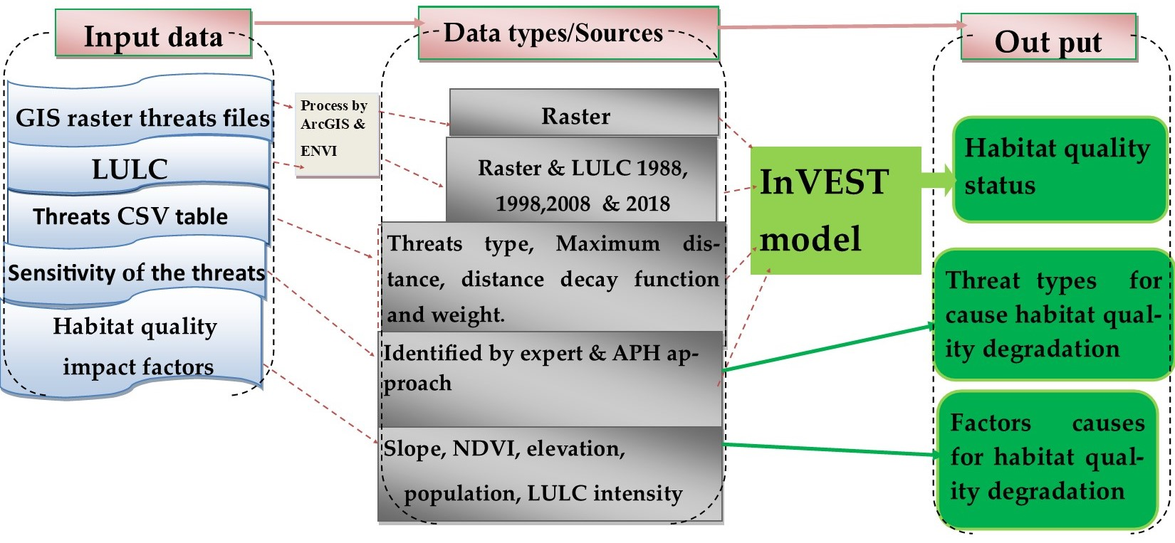
For modeling the habitat quality, different geospatial data parameters were prepared using ArcGIS 10.4 (Table 1). Based on Sharp et al. [32] supported by other research such as Mashizi and Escobedo [6] and Sallustio et al. [63], used data on LULC, the relative weight of each threat (Wr), the habitat sensitivity of each threat (Sjr), the distance between habitats and sources of threats (Max. D), and habitat existence (presence/absence, Hj) to model habitat quality. These parameters were determined using expert knowledge supported by a field survey [7].
Six woredas/districts and twelve villages/kebeles were selected for sampling using systematic random sampling (Table 1) based on Tashakkori and Teddlie [64]. To this end, intensive key informant interviews (KII) were undertaken in 12 villages in the districts with 72 experts (12 experts from each district, who had a good ecological understanding of the watershed) from the Guraghe zone, the environmental protection and natural resource office. The survey was designed according to the method used by Diehl et al. [65] to better understand opinions regarding the importance of specific threats. The respondents were asked to identify the habitat existence/types, as well as the major threats found in the area: Water abstraction, sedimentation, population growth, pollution, invasive species, etc. The maximum distance of the threat affects the habitat quality and distance decay (the threat affects the habitat quickly or slowly) also responded by 72 experts. Next, opinions regarding the major threats’ impact on specific land-use types (forest, woodland, grazing land, shrubland, and cultivated land) were explored using the analytical hierarchy process (APH) model. The APH model was widely used to assign a weight to each threat by examining each threat’s potential impact on the habitat using a pairwise comparison matrix, with 1 to 5 preference scale [66,67] with the following Likert scale values: 5 (very high), 4 (poses a high threat), 3 (poses a medium threat), 2 (poses a low threat), 1 (poses no threat), and 0 (do not know). A matrix was built for each village by using expert-based judgment, containing threats that were used for the pairwise comparisons. Each element’s weight provided by an expert in the matrix was divided by its column total to generate a normalized pairwise matrix. Finally, the weighted matrix (averaging across the rows of the matrix) was generated using the eigen vector (priority vector), which shows each factor’s impact on the habitat [68]. This is vital to assess pairs of threats as alternatives and compare each other in terms of their importance. The corresponding consistency ratio (CR) to verify the acceptable accuracy of pairwise comparisons in a judgment matrix is less than 10% [66]. Finally, the average threat weight/sensitivity values for the 12 villages were used for each land-use type.
Focus group discussion (FGD) were also conducted for triangulation of the data and two clusters of FGD in each district/village were undertaken based on previous studies by Aneseyee et al. [56]. The participants of the FGD, with range of 7 to 10 in one cluster (Table 2) were elder, youth, and female representative, local administrator, and indigenous ecological knowledge person. Open and close ended structured questionnaires were prepared based on Arabatzis et al. [69] to obtain data of habitat types, types of threats for the habitat, distance between threats, and the habitat and sensitivity of the impact to the habitat (see Questionnaire S6 in Supplementary Materials). The fundamental points captured by KII with the experts and FGD include threats types in their surrounding habitat, causes for degradation of the habitat, estimating the maximum distance between the threats and habitat, the spreading rate of the threat (distance decay measurement), sensitivity measurement (which threat has more impact on the habitat), overall status of the habitat quality in their districts, and the types of measures used so far to control the threat for the ecosystem in the study area. Finally, the KII and the interviewees’ responses were collected and organized according to the InVEST habitat quality model requirement with respect to each LULC.
The model also assumes that the more sensitive a habitat type is to a threat (higher Sjr), the more degraded it becomes. In general, the impact of a threat on a habitat decreases as the distance from the degradation source increases and vice versa. Habitats closer to threats have suffered a higher impact, while threats far away from the habitat have a lower impact. Once the maximum effect distance of the threats and the threat impact (disturbance intensity) are determined by consultation, the spatial distribution of threats was determined using interpolation, Euclidian distance, and buffer in ArcGIS for the InVEST habitat quality model.

2.2.2. Data Preparation and Input for the InVEST Model

Cloud-free Landsat satellite images (Table 3), with path = 169, row = 54, for the dry seasons (January to February) for 1988 (Landsat 5), 1998 (Landsat 5), 2008 (Landsat 7), and 2018 (Landsat 8) were obtained from the United States Geological Survey (USGS) data portal (https://earthexplorer.usgs.gov). The spectral band spatial resolution used in this analysis was 30 m, and all the images of the investigated area were cloud free (0%). The images were already terrain-corrected and projected to the Universal Transverse Mercator (UTM) of WGS84 zone 37 N. The images were radiometrically calibrated to the reflectance value, and the Quick Atmospheric Correction algorithm was applied in the ENVI v5.2 software. The supervised image classification method was employed using the Mahalanobis distance classification. The reference data collected using GPS [70] were first converted into a vector file, then into a region of interest (ROI) in the ENVI software. Using the ROI, the spectral signature of each LULC type has been extracted.
Due to the failure of the scan line corrector (SLC) encountered in 2003, the images acquired by the sensor had a data gap (striping) for 2008. Hence, we applied image gap-filling using a ‘gap-filling’ tool in ENVI v5.2 using two images, the acquisition dates of which were only two weeks apart.
A confusion matrix (error matrix) was used to measure the reliability of the LULC classification and validation [71]. The matrix compared the ground true data obtained from reference sites with the classified image results for the sample areas. Thus, the error matrix yielded the overall accuracy, producer and user accuracies, and kappa statistic [72].
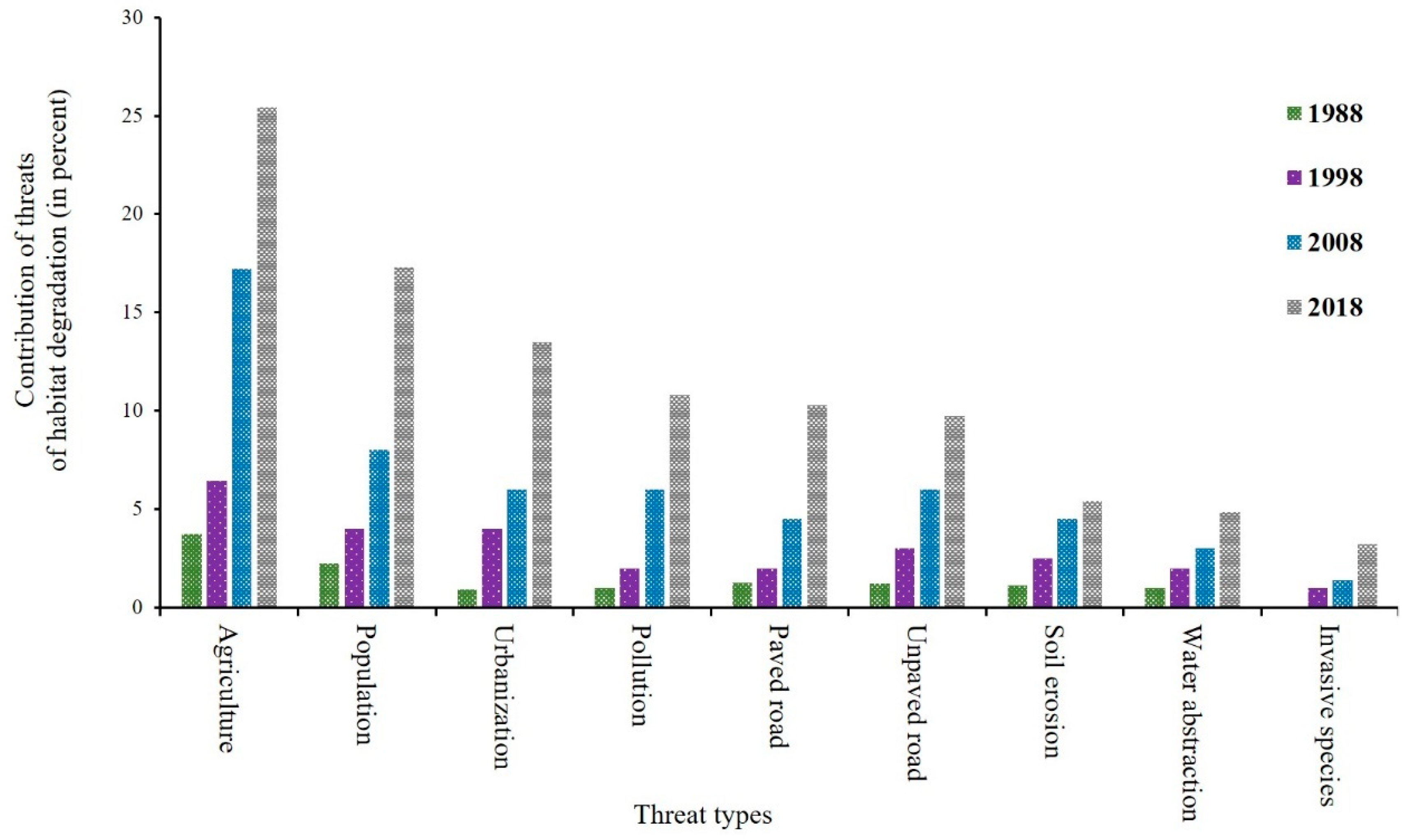
Nine anthropogenic threats were identified in the watershed by following the approach of Terrado et al. [7] and Wu et al. [73]. They were agricultural expansion, invasive species, pollution, soil erosion, urbanization, population growth, water abstraction, and paved and unpaved roads (Table 4). The watershed is one of the most densely populated areas of the country with a maximum estimated population density of 293 people per km2 [74]. What is more, the density follows an increasing trend (Table 5). High population pressure has resulted in an increasing degradation of the natural environment, which disturbs the habitat quality [75]. The population in the Gumer district of the watershed is higher and denser than in the five woredas (districts: Cheha, Ezha, Geta, Merab Azernet, Enemor) (Table 5), which results in more significant habitat degradation. Moreover, the district cities affect biodiversity more than rural areas by generating waste.
The population data provided by the CSA [59] and the 1987 forecast for other years were used with Equation (1) based on Haque et al. [76]:
Nt = P*e(r*t)
where Nt is the forecast population size in a year; P is the population size; e is the natural logarithm to the base e (2.71828); r is the rate of increase (natural increase divided by 100); t is the period involved.
Urbanization increased by 444.73% from 891.23 ha in 1988 to 3963.6 ha in 2018 (Figure 3). Urbanization includes dense settlements, commercial areas, multiple governmental and private institutions, schools, religious institutions, health centers, educational institutions, and other social service areas. Hence, these institutions could generate high waste that is considered a threat to biodiversity and have irreversible environmental effects that affect the quality of the surrounding habitat. However, distance to urbanized areas was considered an important determinant factor for habitat quality rating. Accordingly, the experts recognized that urbanization has a maximum impact of 7 km and it has less impact on the habitat quality at a large distance than at a proximate distance.
According to a Guraghe municipal annual report on waste (m3/month) for Ezha (1624 m3), Cheha (1682 m3), Gumer (1598 m3), Merab Azernet (1534 m3), Gunchre (1512 m3), and Geta (1489 m3), waste generation affects habitat quality up to 20 km causing serious pollution of water bodies, soil, dumping of nonbiodegradable plastic to pristine environment and unpleasant odor. The solid waste is also promoting wildlife and human disease transmission by creating a favorable condition for reproduction of harmful insects and reptiles, bacteria and virus, which might be damaging the grazing land and the vegetation. Dumped solid waste also causes car accidents on the road, illegal open dumps often block the drains and sewers. Strong wind and storms are spreading dust and filth from the open dumps of solid waste to adjacent areas.
Agricultural expansion (Figure 4) is also a threat to biodiversity due to the destruction of the habitat. Vegetation clearing is also likely, hindering the regulating capacity of the land, which results in hampered biodiversity and affects habitat occurrence up to 1 km.
The InVEST sediment delivery model was used to simulate the potential soil erosion in the watershed based on the RUSLE equation of Wischmeier and Smith [77], using six factors (Equation (2)):
RUSLE i = ( R K LS C P ) i
where RUSLE i is the mean annual soil loss (t/ha/year), R is the rainfall erosivity (MJ Mm/ha/year), K is the soil erodibility (MJ mm/t/ha), LS is the topographic factor (dimensionless) (length and gradient), which was generated from DEM, C is cover (dimensionless) simulated by means of normalized difference vegetation index (NDVI), and P is management (dimensionless).
The erosivity factor was calculated using Equation (3), as provided in Hurni [78] and derived from spatial regression analysis for Ethiopian conditions, based on the available mean annual rainfall (P) for thirty-year data of daily and monthly rainfall from meteorological stations in the watershed (Emdiber, Gubre, Gunchre, Agena, and Gumer). Inverse distance weighted interpolation (IDW) was used to create the spatial raster map. The interpolated R factor was used as input for the InVEST model for the year 1988, 1998, 2008, and 2018:
R = −8.12 + 0.562P
where R is the erosivity factor and P is the mean annual rainfall in mm/year.
Based on the Food and Agriculture Organization (FAO) (1984), a soil map of Ethiopia (1:2,000,000), was generated and the shapefile of the legacy soil map was obtained from the FAO and complemented by the Omo-Gibe River Basin master plan soil database, made available by the Ethiopia Water, Irrigation and Electricity Ministry (MOWIE). Five soil types were identified in the study area; Chromic Luvisols, Pellic Vertisols, Eutric Nitosols, Leptosols, and Orthic Acrisols. In each soil type, plot soil samples were taken to determine the K-factor using Equations (4) and (5), based on the four soil characteristics that determine erodibility (sand, clay, silt, and soil organic matter content). The organic matter and soil texture were analyzed at Wolkite soil laboratory by taking 20 soil samples, considering each LULC, from the five soil types (total of 100 samples) of the watershed.
Soil   Erodibility   ( K ) = 2.1 M 1.14 ( 10 4 ( 12 OM ) ) 7.59
where K is soil erodibility, OM is soil organic content (%), and
M = ( ( % silt   +   % sand ) × 100 % clay )
The corresponding average C-value was determined for each LULC class for the years (1988, 1998, 2008, and 2018) based on NDVI value using Equations (5) and (6), following Durigon et al. [79]:
C = ( NDVI + 1 ) 2
NDVI = ( NIR RED ) ( RED + NIR )
where NIR is the surface spectral reflectance in the near-infrared band and RED is surface spectral reflectance in the red band.
The NDVI was computed by processing Landsat images for 1988, 1998, 2008, and 2018 in the ENVI v5.2 software and ArcGIS spatial analysis was used to extract NDVI for each LULC in the reference years. A higher NDVI value indicates higher vegetation cover and vice versa. Moreover, NDVI is determined by a combination of bands based on Landsat images but the formula for using bands over a period of time varies. The 2018 NDVI formula is different from the rest of the years. LANDSAT 5–7 used NDVI = (B4 − B3)/(B3 + B4) for 1988, 1998, and 2008. For 2018, NDVI = (B5 − B4)/(B5 + B4), was used by Landsat 8. Landsat 5 is used for 1988 and 1998, Landsat 7 is used for 2008, and Landsat 8 is used for 2018.
Management practices (P) were determined based on field observation in the upper, middle, and lower watershed, depending on the different conservation practices, and the value of the P-factor ranges from 0 to 1, as suggested by Ganasri and Ramesh [80]. For agricultural lands, the p-value was assigned based on slope classification, using a reclass tool in the ArcGIS software. The mean annual soil loss in the watershed increased from 6.03 t/ha/year in 1988 to 17.91 t/ha/year in 2018 (Figure 5). Soil erosion results in decline in soil fertility in upstream parts of the land affecting farmland at a maximum distance of 2 km. The erosion-based constraint significantly affects the downstream ecosystem degradation such as sedimentation of reservoirs created with dams, the burial of fertile agricultural fields with boulders and stone, etc.
The threat data on invasive species, pollution, water abstract, and road system were not found for 1988, 1998, and 2008. Therefore, the same data were used for 1988, 1998, 2008, and 2018. The spatial distribution threats effect of invasive species and pollution were mapped using IDW interpolation techniques of the ArcGIS whereas road was spatially mapped using buffer and water abstraction delineated using Euclidean distance.
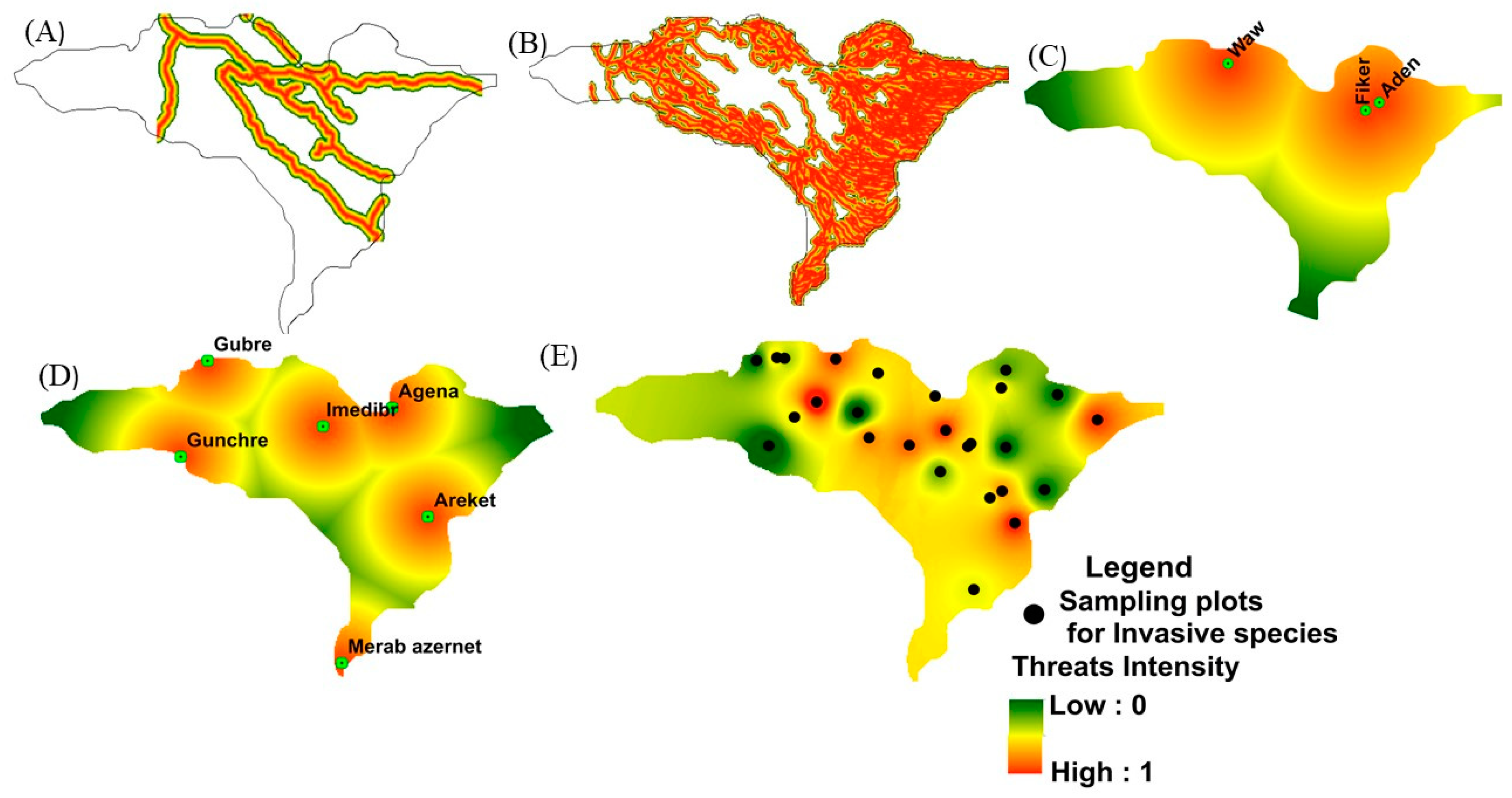
Invasive species are considered a threat to biodiversity, as well due to the possibility of a quick invasion on productive land and their allelopathic effect on the surrounding biodiversity. The authors investigated the density of invasive species by systematic field sampling and count on 20 by 20-m patches on 60 plots. The invasive species were identified by a botanist and using a field manual. They were Senna didemobotrya (50 stems/ha), Parthenium hysterophorus L. (100 stems/ha), Argemone ochroleuca (70 stems/ha), Calitropis procera (80 stems/ha), and Nicotiana glauca (wild tobacco) (48 stems/ha). They were more prevalent on the roadside and near urbanized areas (Figure 6E).
There are three private water abstraction facilities producing drinking water in the watershed, Aden, Fiker, and Waw. They were established after 2012. The amount of water abstracted per year in Aden, Fiker, and Waw was 100, 67, 50 million m3, respectively. This water abstraction affects the ecosystem of the watershed by reducing available water. It further has a significant impact on the downstream Omo-Gibe dams. Therefore, the greater the distance from the water production industry, the greater the persistence of biodiversity in the area and the lesser the sensitivity to the threat.
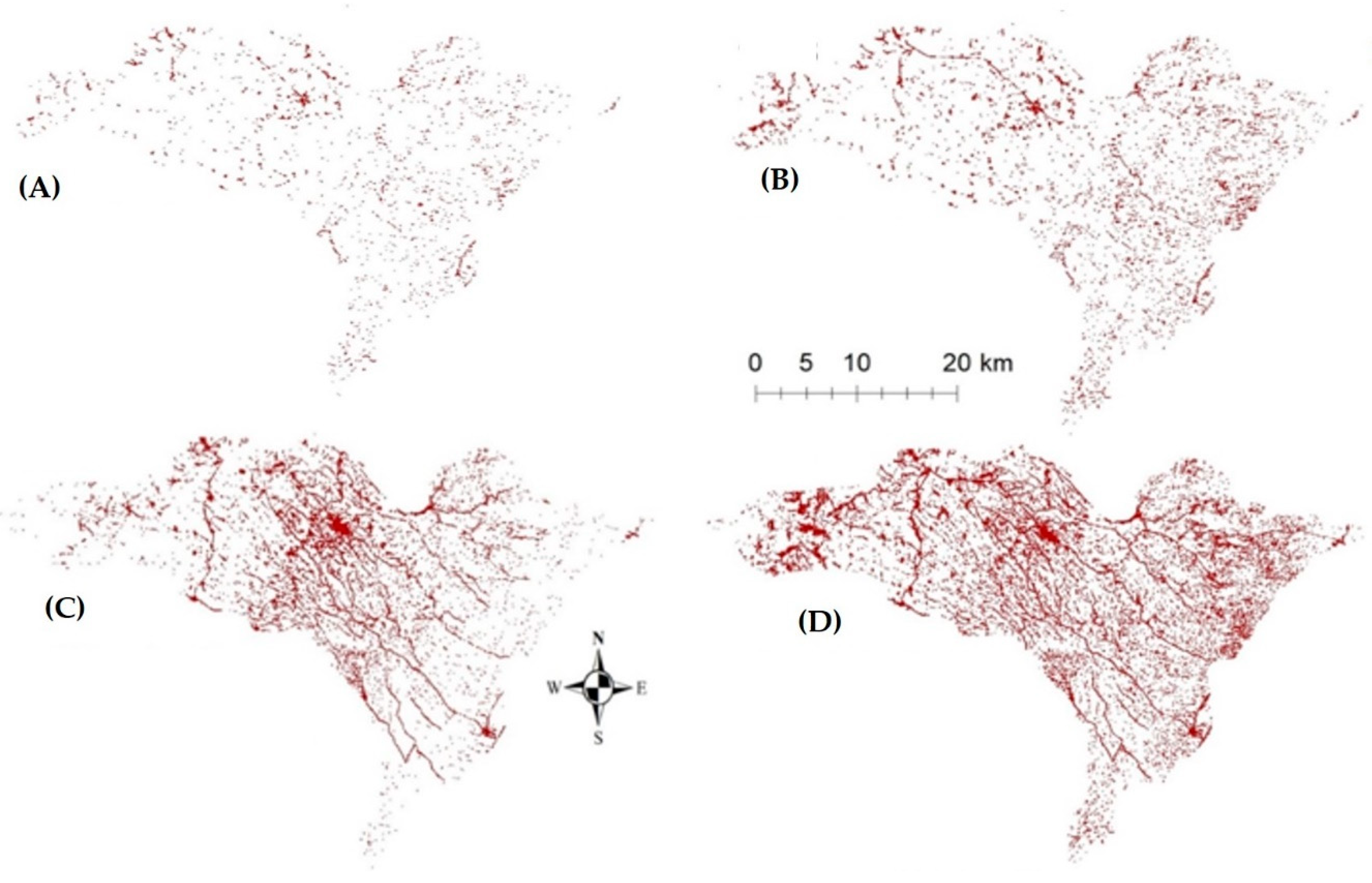
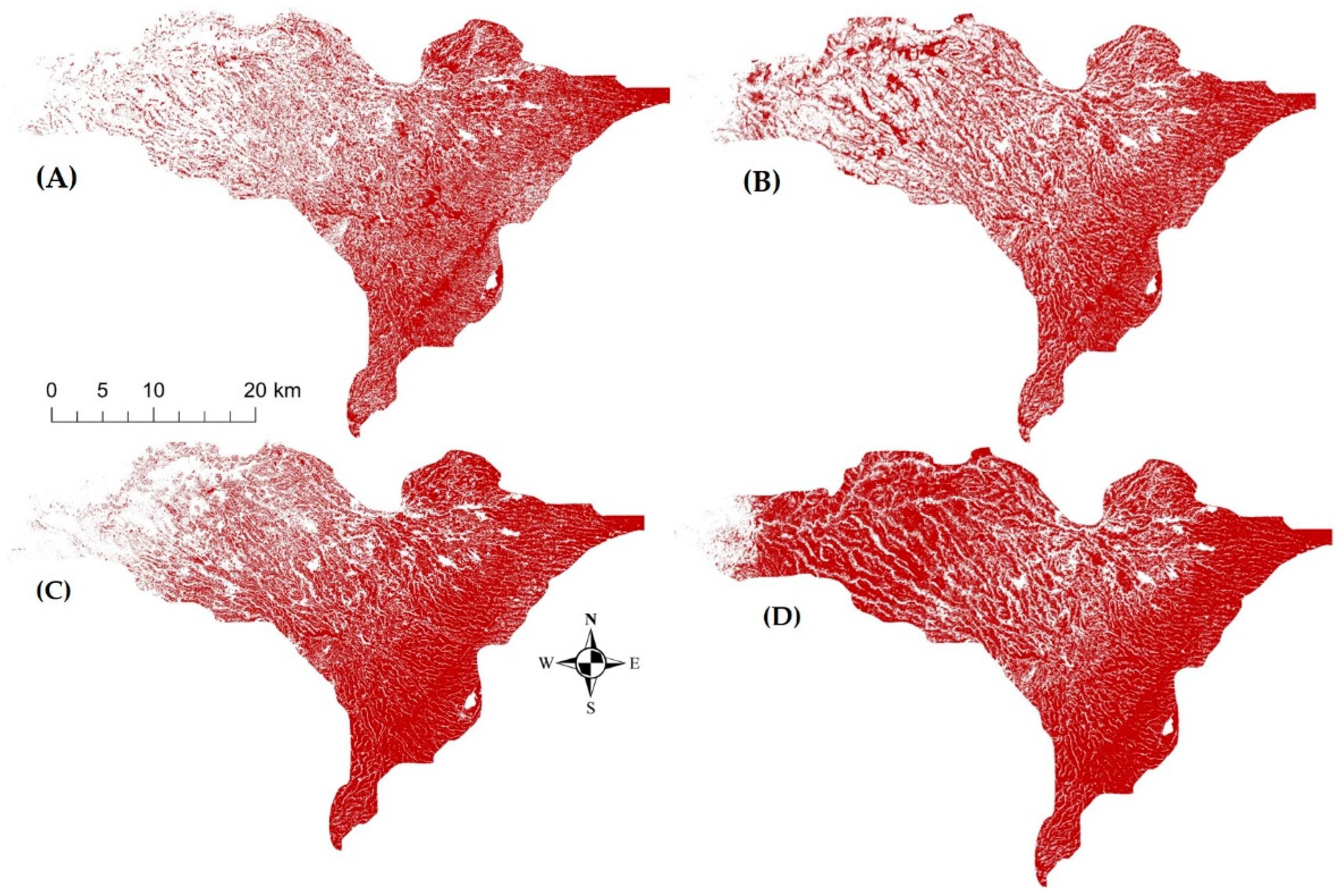
The primary road system has high traffic density (Figure 6A). It becomes a threat to biodiversity because of exhaust gas pollution, soil pollution, noise pollution, and the danger to animals that cross the street. The secondary road system (Figure 6B) also influences the habitat quality by providing transport opportunities for people and animals even though its impact is lower than that of the primary road system. The road system also fosters the timber and nontimber forest product harvesting, which leads to deforestation and disturbance of the habitat quality. Therefore, a primary road is considered a threat to the maximum distance of 1.5 km and a secondary road is assumed to be a threat at a distance up to 0.5 km. The absence of any roads prevents degradation of biodiversity.
The relative habitat suitability score (intensity of the threat) can be assigned to each LULC type, ranging from 0 to 1, where 1 indicates the highest habitat suitability and 0 indicates the lowest suitability [36,48]. Threats and sensitivity scores were determined based on literature data and expert knowledge (Table 6).
The InVEST model is used as a half-saturation curve to show the relationship between habitat degradation scores and habitat quality scores [81]. Threat decay in space is described as either a linear (Equation (8)) or exponential (Equation (9)) distance-decay function. The InVEST model determines the impact of threat r that originates in grid cell y, ry, on habitat in grid cell x as irxy in Equation (8):
if   linear ,   i rxy = 1 ( d x y d r   m a x )
if   exponential ,   i rxy = e x p ( ( 2.99 d r   m a x ) d x y )
where dxy is the linear distance between grid cells x and y and dr max is the maximum effective distance of threat r’s reach in space.
The total threat level in grid cell x with LULC or habitat type j is determined with Equation (10):
D x j = r = 1 R y = 1 Y r ( w r r = 1 R W r ) r y i r x y β x S J r
where r is the LULC threat, with r = 1, 2,…n; R is the index of all the modeled degradation sources; y is the index of all grid cells on r’s raster map; Yr indicates the set of grid cells on r’s raster map; wr are the weight parameters; βx is the accessibility factor.
The quality of habitat (Qxj) in parcel x or LULC j is calculated with Equation (11):
Q x j = H j ( 1 ( D x j z D x j z + k z ) )
where Hj is each LULC assigned a habitat score from 0 to 1 (1 = highest habitat suitability, 0 = no habitat), z = 2.5 and k are scaling parameters (or constants). The k constant is 0.5.
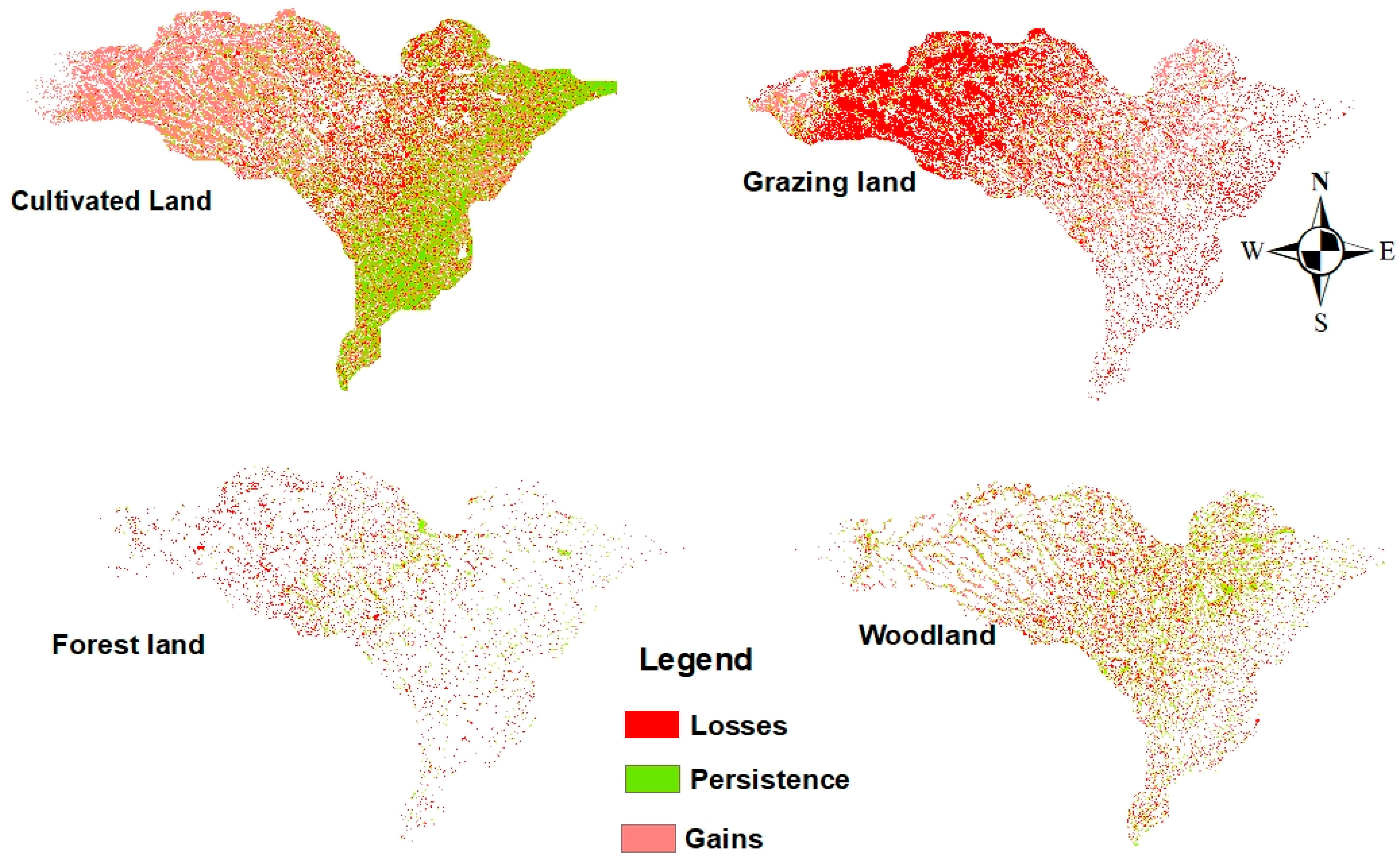
The LULC area for 1988, 1998, 2008, and 2018 has been drafted (Table 7). The land has been classified into eight classes with a numeric LULC code for each class: Bare land (1), built-up land (2), shrubland (3), cultivated land (4), forests (5), grazing land (6), water bodies (7), and woodland (8). The LULC raster encompasses the area of interest and a buffer the width of which is the greatest maximum threat distance.

2.2.3. Correlation Analysis of Habitat Quality and Impact Factors

The analysis of correlation demonstrates that the investigated factors had an impact on habitat quality. It employed the impact factors of anthropogenic origin (LULC intensity and population density) and those related to physical geography (elevation, slope, and NDVI). The correlation was examined for 150 sub-watersheds, delineated based on the altitude and drainage density, using ArcSWAT. The habitat quality and relevant impact factors were explored using spatial analysis in ArcGIS 10.4.
The LULC intensity reflects the extent of disturbance caused by anthropogenic activity in a sub-watershed. According to Hu et al. [82], human activities that disturb land use/land cover have different levels of intensity, as shown in Table 7.
The NDVI average data for January for the reference’s year (1988, 1998, 2008, and 2018) were used from the USGS because it reflected the distribution of natural vegetation in the dry season. A higher value of the NDVI indicates that the area has a good vegetative cover, while a lower value indicates nonvegetation, and thus a nonhabitat. The NDVI values were high for forests (0.31), woodland (0.29), grazing land (0.11), and shrubland (0.13) and low for cultivated land (−0.01), built-up land (−0.27), and bare land (−0.38). Slope and elevation data were taken from a digital elevation model (DEM) with resolution of 30 m and version 3 downloaded from the ASTER GLOBAL DEM site (https://earthexplorer.usgs.gov).

2.2.4. Statistical Analyses

Pearson correlation analysis was performed using the R 3.2 software at a significance level of p < 0.01. It is expressed by the coefficient r between −1 and +1, and it measures the linear relationship between two variables (dependent and independent one) with the R script cor (). If the r value approaches negative 1, the habitat quality and the independent variable increases inversely proportionally (habitat quality increases whereas the factor decreases). With r approaching positive 1, the habitat quality increases as the factor increases. Multiple collinearities between the variables can be checked using the R software with a package of variance inflation factor (VIF) function. It provides an index that measures how much the variance of an estimated regression coefficient is increased because of collinearity. This shows which factor is a more influential driver of the habitat quality degradation. For VIF > 10 there are multiple collinearities between the variables but its impact on the habitat quality is insignificant. If it is less than 10 or approaching zero, the factor impact on the habitat quality is significant.
Box-Cox transformation is defined a measure of the normality of the resulting transformation data. The Box-Cox normality plot is a plot of the correlation coefficients for various values of the λ parameter. The value of λ corresponding to the maximum correlation on the plot is then the optimal choice for λ. Box-Cox transformation is defined as T ( Y ) = ( Y γ 1 ) / γ , where Y is the response variable and γ is the transformation parameter. ArcGIS 10.4 was also used to analyze spatial and temporal changes in habitat quality by subtracting first-year values from last-year values.

3. Results

3.1. Land Use/Cover Changes Associated with the Threats

The land-use pattern in the Winike watershed has changed dramatically in the past 30 years. The vegetation cover declined significantly by 177.43%, while agricultural land and built-up land expanded significantly from 1988 to 2018 by 133.01% and 444.73%, respectively (Table 8). The increase in cultivated land resulted in the threat of soil erosion and the decline of vegetation cover. As a result of the declining forest, shrub, and grazing land areas, the forest land, shrubland, and grazing land habitat types also decreased. Moreover, increasing urbanization resulted in increasing pollution accumulation, which affected habitat quality significantly.
The matrix of LULC from 1988 to 2018 showed that cultivated land remained unchanged in 29.13% of sub-watersheds, grew in 13.59% and declined in 22.09% in the last 30 years. The grazing land was lost in 14.79% of sub-watersheds, increased in 14.59%, and persisted in 3.66%. Forests persisted in 2.12% of sub-watersheds, grew in 1.56%, and declined in 3.4% (Figure 7). The woodland also declined in 0.70% of sub-watersheds, increased in 0.72%, and persisted in 9.24%.
The overall accuracy for the land use classification was 85.23% in 1988 and 95.30% in 2018. The kappa coefficient ranged from 0.88 in 1988 to 0.93 in 2018, showing a high level of agreement between the classified image and the referenced data. The error matrix showing the producer and user accuracies of the 1988 Landsat classified image for the land-use types was lower compared to the 2018 Landsat classified image due to the image quality difference (Table 9).

3.2. The Threat Sources and Their Contribution to Habitat Degradation

Agricultural expansion, population, pollution, urbanization, primary and secondary road systems, water abstraction, and invasive species were the most significant sources of the threat of habitat degradation (Figure 8). The worst among these was agricultural expansion. Its threat proportion increased from 3.75% in 1988 to 25.41% in 2018. The habitat degradation threat from population pressure increased from 2.22% in 1988 to 17.3% in 2018. However, water abstraction and invasive species contributed little to the degradation of habitat quality (<5%) compared to the remaining threat types. Nevertheless, each threat factor’s impact and sensitivity to threats have increased over the last 30 years (1988 to 2018).

3.3. Changes in Habitat Quality in the Watershed

The habitat quality has declined in the watershed over the past 30 years, with an average score of 0.41 in 1988, 0.35 in 1998, 0.30 in 2008, and 0.23 in 2018. The red color in Figure 9 indicates the degradation of habitat in the respective years. The phenomenon dominates in the eastern part of the watershed. This is due to the increasing impact of threat factors of anthropogenic origin. The green color shows high habitat quality found in the central and downstream parts of the watershed. The red color increased while the green color declined from 1988 to 2018, which indicates that the quality of habitat has degraded.
The biodiversity high suitability area was 33.12 thousand ha (30.34% of the watershed) in 1988. It declined to 16.19 thousand ha (14.83%) in 2018. The area of medium suitability for habitats decreased by 23.85%, while low habitat quality area significantly increased from 26.83% in 1988 to 66.19% in 2018 (Table 10). This shows that the pristine habitat area has decreased due to the increase in threat factors affecting the ecosystem of the watershed.
Moreover, the rate of change in habitat quality and degradation was more severe recently, from 2008 to 2018, as compared to the periods from 1998 to 2008 and from 1988 to 1998. This indicates that the social, economic, and natural causes of habitat degradation have increased recently.
A significant change in the spatial distribution and variability of habitat quality in each LULC type of the Winike watershed together with habitat quality analysis of the land-use pattern shows a decreasing trend (Figure 10), i.e., habitat quality in cultivated land, forests, woodland, grazing land, shrubland, and water bodies followed by a negative trend. The lowest habitat quality (0) or nonhabitat was observed for bare land and built-up land, while the highest habitat quality (1) was mainly found in forests, grazing land, and shrubland. However, the conversion of habitat types into nonhabitat types from 1988 to 2018 was 39.21% of the Winike watershed.
The average habitat quality of forests and shrubland were 0.777 and 0.507, respectively (Table 11), which was more than the other LULC types. Low habitat quality in bare land, built-up land, cultivated land, and water bodies indicates low habitat/biodiversity suitability. The Gibe Sheleko National Park in the downstream (western) part of the watershed contributed to high biodiversity due to a suitable habitat. The habitat suitability in the upstream (eastern) part of the watershed is lower due to high habitat vulnerability to anthropogenic activities such as continued crop cultivation, dense population and urbanization, expansion of invasive species, the substitution of indigenous trees by eucalyptus plantations, and deforestation. Therefore, the eastern part of the watershed has a higher habitat quality than its western part.

3.4. The Impact Factors for Spatial Patterns of Habitat Quality

The factors, such as anthropogenic activities and physio-geographical factors (Table 12), have influenced the spatial patterns of habitat quality in the watershed and each impact factors frequency distribution were given in Figure 11.
The statistical analysis (Figure 12) indicated that elevation was significantly correlated with the distribution of habitat quality (r = −0.43, p < 0.01) in the Winike watershed over the 30 years (Table 13). Due to the high elevation and gentle slopes, the eastern part of the watershed offered favorable conditions for the expansion of intensive agriculture and continuous annual cereal crop cultivation, which led to a high impact and fragmentation of the habitat quality. However, due to the low elevation and undulating topography, habitat suitability was high in the western part of the watershed where Gibe Sheleko National Park is situated. This area contributes to biodiversity conservation by creating a favorable habitat. Therefore, this shows that the habitat quality is high in the downstream (western) part of the watershed, and low upstream.
The NDVI was significantly correlated with habitat quality of the reference years (r2018 = −0.14, r2008 = 0.13, r1998 = 0.11, p < 0.01) but nonsignificant (r1988 = 0.01) for the year of 1988 (Table 13). This indicates that the watershed had high habitat quality and vegetation cover to foster biodiversity in 1988, but they declined in time.
The correlation between habitat quality and population density was significant for the year 2018 and 2008 (r = −0.1 and r = −0.09, respectively) but nonsignificant for the two previous reference years (1998 and 1988) (r = −0.04 and r = −0.01, respectively). This shows that anthropogenic activities had a significant effect on the fragmentation of habitat quality and biodiversity. Moreover, habitat quality in and around urban areas was lower due to the high population density and intensive economic activity. This leads to the disturbance of the habitat through such factors as pollution, deforestation, or expansion of agriculture.
The correlation between the intensity of land use and habitat quality was significant for the three reference years (1998, 2008, and 2018) but nonsignificant for 1988 (Table 13). It was because the exploitation of land resources, which affected habitat quality, was greater more recently than previously.
The collinearity analysis show that, higher values of VIF indicate it is difficult or even impossible to assess accurately the impact contribution to the habitat quality. Therefore, the impact of factors such as population, NDVI, and intensity of land use on the habitat quality increased over a period of time as shown in Table 14, whereas slope and altitude effect exhibited a constant impact throughout the period. The VIF of population in 1988 and 2018 was 0.89 and 0.12, respectively. This indicates that the contribution of population pressure for the degradation of habitat quality is higher in 2018 as compared to 1988.
The Box-Cox normality plot (Figure 13) of the habitat quality shows that the maximum value of the coefficient is 0.2 at λ = −0.2. The data of the Box-Cox transformation with λ = −0.2 shows a data set for which the normality assumption is reasonable.

4. Discussion

The results of this study indicate that the land-use pattern in the Winike watershed has changed rapidly and dramatically during the past 30 years. This was mainly due to the Agricultural Development Lead Industrialization (ADLI) policy of Ethiopia. The policy promoted intensive farming practices and cropland expansion through the extension of credit, improved seeds, and chemical fertilizers. The aid encouraged farmers to implement intensive agricultural practices, which contributed to the clearing of indigenous vegetation and the habitat quality. This, in turn, contributed to the degradation of the natural forest and pristine environment in search of land [83] and has been reported to happen in many tropical regions [84].
The central and western parts of the Winike watershed have better habitat quality than the eastern part, which promoted biodiversity and environmental regulation in the watershed. However, the booming population, agricultural expansion, and urbanization posed threats to habitat quality [49], and led to a decline of habitat quality in the watershed. The sources of the threats are more severe in the eastern part of the watershed than in its western part. For example, Gumer, Merab Azernet, and Geta are administrative areas in the eastern part of the watershed with a high population per km2 compared to Enemore, Cheha, and Ezha (western part). Due to population pressure, such threats to habitat quality as soil erosion, urbanization, pollution, or agricultural expansion increased.
The agricultural expansion could decrease biodiversity in the watershed due to the continuous farming of cereal crops, particularly in the eastern part (Gumer, Merab Azernet, and Geta districts). However, the western and central parts (Enemore, Cheha, and Ezha district areas) of the watershed employ different agroforestry practices and have more varied vegetation cover. As a result, the habitat quality is low in the eastern part of the watershed compared to its western part. Sun et al. [85] confirmed that intensive local agricultural activity directly impacts habitat quality and biodiversity.
The existence of protected areas in the watershed contributed significantly to alleviating habitat quality in the area [86]. The Gibe Sheleko National Park was established in 2003 to conserve the biodiversity in the upper Omo-Gibe Basin. Some parts of the park stretch out into the Winike watershed. Therefore, the western part of Winike watershed is covered by the park and benefits from its contribution to the regulation and conservation of habitat quality.
The InVEST habitat model can be used to estimate and juxtapose the relative impact of threats to identify threats that are more damaging to the biodiversity in a specific landscape of the investigated watershed. For example, agricultural land-use types could be sensitive to threats generated by soil erosion but less sensitive to threats generated by paved road systems. This means that the impact of soil erosion on cultivated land is higher compared to paved road systems. Forest land-use type is more sensitive to the threat of agricultural expansion than other threats such as soil erosion or invasive species. The study assessed habitat quality threats and habitat sensitivity to threats in the field based on the InVEST habitat quality model according to guidelines developed by Sharp et al. [32,36]. Thus, the habitat quality threats identification and sensitivity analysis for the Winike watershed were consistent with the study by Baral et al. [87].
Among the types of threats to habitat quality, the expansion of agricultural land significantly contributed to the degradation of habitat quality (1988 = 3.75%, 1998 = 6.45%, 2008 = 17.23%, 2018 = 25.41%). This is consistent with studies by Dai et al. [1] and Petit et al. [88] who demonstrated that agricultural expansion is the cause of clearing of large areas of indigenous vegetation, which results in fragmentation and loss of habitat and biodiversity [89].
Road systems can be considered a threat as they can facilitate anthropogenic disturbance, logging, and overexploitation by improving access to markets [90]. More than 95% of Amazonian deforestation occurs within 50 km of a road. Keeping roads out of natural habitats is the most effective approach to environmental protection there [91]. The investigated watershed has patches of natural forests such as Kotergedera, Genemar, Yoteyet, Zaram, Ambeli, and Kubena, but they are degrading due to accessibility of infrastructure development such as roads.
The changes in the Boye wetland of Jimma, Ethiopia reduced the avifauna population and species composition [92]. This statement is consistent with the findings of this study, which indicates that biodiversity differs according to changes in ecological characteristics and that different species exhibit varying responses to changes in habitat. Thus, the alteration in the ecosystem in the form of LULC changes has harmed its biodiversity.

4.1. Limitations of Uncertainty and Future Recommended Works

The practical application of the InVEST habitat quality model remains limited, although it is an important tool for landscape managers to conserve biodiversity [32]. In the investigated site, we have noticed that there are no long-term quantitative data about habitat quality and its threat factors. Therefore, the quadrant species collection is an important indicator for the validation of the model results. Note the lack of research on InVEST habitat quality modeling associated with the LULC change in the Omo-Gibe Basin, Ethiopia, and east Africa.
The soil, climate, hydropower generation, edge effect, and vegetation difference of the habitat had a little impact recognized by the InVEST habitat quality model [93]. Furthermore, this type of habitat quality research generally depends on InVEST model dataset parameters and experts’ knowledge or opinion [7,87], since the InVEST habitat quality model requires threat’s maximum effective distance and weights of each ecological threat factor. As a result, the InVEST habitat quality model might be severely affected by the expert’s judgment, which is one of the limitations and potential for future improvement of the model.
The limited availability of geospatial information with time-series data might result in some faultiness and uncertainty of habitat quality assessment and mapping. For example, the same spatial threat data for road, pollution, invasive species, and water abstraction were used for the reference years (1988, 1998, 2008, and 2018). Hence, this aspect needs to be taken care of to improve research finding in the future.
One of the limitations of the InVEST habitat quality model is poor information about species distribution in the landscape [48]. Consequently, this finding provides little further information about the biotic environment (such as animal, plant, and insect biodiversity, etc.). Despite this, the present study had explicitly provided the status and change of biodiversity (habitat quality) by amalgamation of GIS and ecological data. Therefore, in order to conduct convincing habitat quality modeling and mapping using the InVEST model, it is not enough to use earth observation such as satellite tracking and remote sensing, but other model simulations and quadrant measurements of species have to be employed in future research [94,95,96,97,98]. For example, the FRAGSTATS 4.2 model can analyze such landscape habitat quality parameters as patch density, splitting index, Shannon’s diversity index, Shannon’s evenness index, and the largest patch index [1]. If this model is applied in the study of the watershed, the uncertainty of the InVEST habitat quality model can be shown.

4.2. Implications of Habitat Quality Modeling

Modeling habitat quality helps prioritize the landscape for the conservation of biodiversity [29]. This research is undertaken for the Omo-Gibe Basin in Ethiopia and the research on the biodiversity of the area is limited. Conducting this research is important as it can encourage more research projects because it shows the ecological risk caused mostly by anthropogenic factors as a side effect of the effort to save time, energy, funds, and manpower.
The Omo-Gibe Basin of Ethiopia is endowed with a high-water resource potential; as a result, the government of Ethiopia has been encouraging the construction of more than three dams, which contribute significantly to the Ethiopia’s green economy. However, the area suffers from potential threats of climate change, population pressure, pollution, deforestation, sedimentation, high surface runoff, and disturbance of stream flow regimes [99]. In order to address these challenges, habitat quality modeling can provide useful information for decision makers since it provides site-specific information on the biodiversity status to implement holistic approaches by stakeholders for conservation and sustainable development in the study area. This information gives insight into where the biodiversity is more degraded, the cause of the degradation (threat), and the sensitivity of the habitat to biodiversity threats. Generally, the research findings are important for showing the need for ecological restoration associated with the LULC change [100] and the profound impact of anthropogenic threats (sedimentation, pollution, roads, etc.) on the existing habitats (biodiversity). This research also helps with land-use planning to implement short- and long-term development projects in order to insure the sustainability of the ecosystem, particularly the dams. Hence, this research is important to realize multiple win-win solutions of the economic, social, and ecological protection and for the sustainable development in the study watershed.

5. Conclusions

The results show that there has been a significant LULC change in the study area over the past three decades (1988 to 2018). In this period, the LULC change has been growing, declining the habitat quality in the Winike watershed. Notably, the vegetation cover has decreased rapidly and agricultural activity has increased. This could be due to increasing anthropogenic disturbance, which results from the snowballing food and resource consumption, promoting damage to the natural environment, and disturbance of the habitat.
The findings indicated that habitat quality degradation was mainly caused by agricultural expansion, population pressure, urbanization, accessibility to road systems, soil erosion, water abstraction, and pollution. The habitat quality in the Winike watershed was distributed mainly downstream (western part) and in the central part of the watershed. To improve the habitat quality in the watershed, it is suggested that land management strategies should be realized according to the severity and extent of habitat quality degradation. This requires urgent biodiversity conservation and control actions in this location.

Supplementary Materials

The following are available online at https://www.mdpi.com/2072-4292/12/7/1103/s1, Table S1: Habitat quality threats factors impact weight analysis (2018), Table S2: Habitat quality threats factors impact weight analysis (1988), Table S3: The maximum distance (d-max) of the threat affect the habitat quality, Table S4: Threats impact distance decay function, Table S5: The habitat threats, their weight, maximum distance and decay for 1988,1998, 2008 and 2018, Questionnaire S6: Survey data gathering questionnaires.

Author Contributions

Conceptualization: A.B.A. and T.N.; methodology: A.B.A., T.N., T.S., and E.E.; software: A.B.A.; validation: T.N., T.S., and E.E.; formal analysis: A.B.A.; investigation: T.S.; resources: T.S., and E.E.; data curation: T.N.; writing—original draft preparation: A.B.A.; writing—review and editing: T.N.; visualization: A.B.A., T.N., T.S., and E.E.; supervision: T.S., and E.E.; project administration: T.S., and E.E.; funding acquisition: T.N., T.S., and E.E. All authors have read and agreed to the published version of the manuscript.

Funding

This research was funded by CASCAPE project in Ethiopia, thematic research of Addis Ababa University, linguistic support was funded by University of Agriculture in Krakow, and the APC was funded by University of Agriculture in Krakow.

Acknowledgments

The authors wish to thank the native English speaker for linguistic support and the specialist from the professional language service agency. The authors would also like to express their gratitude to the editor and three anonymous reviewers for their thorough work with the manuscript and for providing constructive and insightful comments on this paper.

Conflicts of Interest

The authors declare no conflict of interest.

References

  1. Dai, L.; Li, S.; Lewis, B.J.; Wu, J.; Yu, D.; Zhou, W.; Zhou, L.; Wu, S. The influence of land use change on the spatial–temporal variability of habitat quality between 1990 and 2010 in Northeast China. J. For. Res. 2019, 30, 2227–2236. [Google Scholar] [CrossRef]
  2. Rands, M.R.W.; Adams, W.M.; Bennun, L.; Butchart, S.H.M.; Clements, A.; Coomes, D.; Entwistle, A.; Hodge, I.; Kapos, V.; Scharlemann, J.P.W.; et al. Biodiversity conservation: Challenges beyond 2010. Science 2010, 329, 1298–1303. [Google Scholar] [CrossRef] [PubMed] [Green Version]
  3. Ellis, E.C.; Pascual, U.; Mertz, O. Ecosystem services and nature’s contribution to people: Negotiating diverse values and trade-offs in land systems. Curr. Opin. Environ. Sustain. 2019, 38, 86–94. [Google Scholar] [CrossRef]
  4. Watson, K.B.; Galford, G.L.; Sonter, L.J.; Koh, I.; Ricketts, T.H. Effects of human demand on conservation planning for biodiversity and ecosystem services. Conserv. Biol. 2019, 33, 942–952. [Google Scholar] [CrossRef] [PubMed] [Green Version]
  5. Wu, Y.; Tao, Y.; Yang, G.; Ou, W.; Pueppke, S.; Sun, X.; Chen, G.; Tao, Q. Impact of land use change on multiple ecosystem services in the rapidly urbanizing Kunshan City of China: Past trajectories and future projections. Land Use Policy 2019, 85, 419–427. [Google Scholar] [CrossRef]
  6. Mashizi, A.K.; Escobedo, F.J. Socio-ecological assessment of threats to semi-arid rangeland habitat in Iran using spatial models and actor group opinions. J. Arid Environ. 2020, 177, 104136. [Google Scholar] [CrossRef]
  7. Terrado, M.; Sabater, S.; Chaplin-Kramer, B.; Mandle, L.; Ziv, G.; Acuña, V. Model development for the assessment of terrestrial and aquatic habitat quality in conservation planning. Sci. Total. Environ. 2016, 540, 63–70. [Google Scholar] [CrossRef] [Green Version]
  8. Gaglio, M.; Lanzoni, M.; Nobili, G.; Viviani, D.; Castaldelli, G.; Fano, E.A. Ecosystem services approach for sustainable governance in a brackish water lagoon used for aquaculture. J. Environ. Plan. Manag. 2019, 62, 1501–1524. [Google Scholar] [CrossRef]
  9. Adger, W.N.; Adams, H.; Kay, S.; Nicholls, R.J.; Hutton, C.W.; Hanson, S.E.; Rahman, M.M.; Salehin, M. Ecosystem Services, Well-Being and Deltas: Current Knowledge and Understanding. In Ecosystem Services for Well-Being in Deltas; Nicholls, R.J., Hutton, C.W., Adger, W.N., Hanson, S.E., Rahman, M.M., Salehin, M., Eds.; Springer: Palgrave Macmillan, Cham, 2018; pp. 3–27. [Google Scholar]
  10. Wu, J.; Cao, Q.W.; Shi, S.Q.; Huang, X.L.; Lu, Z.Q. Spatio-temporal variability of habitat quality in Beijing-Tianjin-Hebei Area based on land use change. Ying yong sheng tai xue bao = J. Appl. Ecol. 2015, 26, 3457–3466. [Google Scholar]
  11. WHO. Ecosystems and Human Well-Being: Health Synthesis: A Report of the Millennium Ecosystem Assessment. 2005. Available online: http://afrohun.org/ (accessed on 10 May 2019).
  12. Zhao, G.; Liu, J.; Kuang, W.; Ouyang, Z.; Xie, Z. Disturbance impacts of land use change on biodiversity conservation priority areas across China: 1990–2010. J. Geogr. Sci. 2015, 25, 515–529. [Google Scholar] [CrossRef] [Green Version]
  13. Postek, P.; Leń, P.; Stręk, Ż. The proposed indicator of fragmentation of agricultural land. Ecol. Indic. 2019, 103, 581–588. [Google Scholar] [CrossRef]
  14. Gao, Y.; Ma, L.; Liu, J.; Zhuang, Z.; Huang, Q.; Li, M. Constructing ecological networks based on habitat quality assessment: A case study of Changzhou, China. Sci. Rep. 2017, 7, 46073. [Google Scholar] [CrossRef] [PubMed]
  15. Kazak, J.K.; Chruściński, J.; Szewrański, S. The development of a novel decision support system for the location of green infrastructure for stormwater management. Sustainability 2018, 10, 4388. [Google Scholar] [CrossRef] [Green Version]
  16. Kazak, J.; van Hoof, J. Decision support systems for a sustainable management of the indoor and built environment. Indoor Built Environ. 2018, 27, 1303–1306. [Google Scholar] [CrossRef] [Green Version]
  17. Randin, C.F.; Ashcroft, M.B.; Bolliger, J.; Cavender-Bares, J.; Coops, N.C.; Dullinger, S.; Dirnböck, T.; Eckert, S.; Ellis, E.; Fernández, N.; et al. Monitoring biodiversity in the Anthropocene using remote sensing in species distribution models. Remote Sens. Environ. 2020, 239, 111626. [Google Scholar] [CrossRef]
  18. Mahecha, M.D.; Gans, F.; Sippel, S.; Donges, J.; Kaminski, T.; Metzger, S.; Migliavacca, M.; Papale, D.; Rammig, A.; Zscheischler, J. Detecting impacts of extreme events with ecological in situ monitoring networks. Biogeosciences 2017, 14, 4255–4277. [Google Scholar] [CrossRef] [Green Version]
  19. Verburg, P.H.; Crossman, N.; Ellis, E.; Heinimann, A.; Hostert, P.; Mertz, O.; Nagendra, H.; Sikor, T.; Erb, K.-H.; Golubiewski, N.; et al. Land system science and sustainable development of the earth system: A global land project perspective. Anthropocene 2015, 12, 29–41. [Google Scholar] [CrossRef] [Green Version]
  20. Klein, T.; Randin, C.; Körner, C. Water availability predicts forest canopy height at the global scale. Ecol. Lett. 2015, 18, 1311–1320. [Google Scholar] [CrossRef]
  21. Garonna, I.; de Jong, R.; Stockli, R.; Schmid, B.; Schenkel, D.; Schimel, D.; Schaepman, M.E. Shifting relative importance of climatic constraints on land surface phenology. Environ. Res. Lett. 2018, 13, 024025. [Google Scholar] [CrossRef] [Green Version]
  22. Schneider, F.D.; Leiterer, R.; Morsdorf, F.; Gastellu-Etchegorry, J.-P.; Lauret, N.; Pfeifer, N.; Schaepman, M.E. Simulating imaging spectrometer data: 3D forest modeling based on LiDAR and in situ data. Remote Sens. Environ. 2014, 152, 235–250. [Google Scholar] [CrossRef]
  23. Naumann, G.; Barbosa, P.; Carrao, H.; Singleton, A.; Vogt, J. Monitoring drought conditions and their uncertainties in Africa using TRMM data. J. Appl. Meteorol. Climatol. 2012, 51, 1867–1874. [Google Scholar] [CrossRef] [Green Version]
  24. Ibrahim, S.A.; Balzter, H.; Tansey, K.; Tsutsumida, N.; Mathieu, R. Estimating fractional cover of plant functional types in African savannah from harmonic analysis of MODIS time-series data. Int. J. Remote Sens. 2018, 39, 2718–2745. [Google Scholar] [CrossRef]
  25. Janus, J.; Bozek, P. Land abandonment in Poland after the collapse of socialism: Over a quarter of a century of increasing tree cover on agricultural land. Ecol. Eng. 2019, 138, 106–117. [Google Scholar] [CrossRef]
  26. Liu, Y.; Huang, X.; Yang, H.; Zhong, T. Environmental effects of land-use/cover change caused by urbanization and policies in Southwest China Karst area–A case study of Guiyang. Habitat Int. 2014, 44, 339–348. [Google Scholar] [CrossRef]
  27. Guo, Z.; Zhang, L.; Li, Y. Increased dependence of humans on ecosystem services and biodiversity. PLoS ONE 2010, 5, e13113. [Google Scholar] [CrossRef]
  28. Ahrends, A.; Hollingsworth, P.M.; Ziegler, A.D.; Fox, J.; Chen, H.; Su, Y.; Xu, J. Current trends of rubber plantation expansion may threaten biodiversity and livelihoods. Glob. Environ. Chang. 2015, 34, 48–58. [Google Scholar] [CrossRef]
  29. Gong, J.; Xie, Y.; Cao, E.; Huang, Q.; Li, H. Integration of InVEST-habitat quality model with landscape pattern indexes to assess mountain plant biodiversity change: A case study of Bailongjiang watershed in Gansu Province. J. Geogr. Sci. 2019, 29, 1193–1210. [Google Scholar] [CrossRef] [Green Version]
  30. Boykin, K.G.; Kepner, W.G.; Bradford, D.F.; Guy, R.K.; Kopp, D.A.; Leimer, A.K.; Samson, E.A.; East, N.F.; Neale, A.C.; Gergely, K.J. A national approach for mapping and quantifying habitat-based biodiversity metrics across multiple spatial scales. Ecol. Indic. 2013, 33, 139–147. [Google Scholar] [CrossRef]
  31. Hooper, D.U.; Chapin, F.S.; Ewel, J.J.; Hector, A.; Inchausti, P.; Lavorel, S.; Lawton, J.H.; Lodge, D.M.; Loreau, M.; Naeem, S.; et al. Effects of biodiversity on ecosystem functioning: A consensus of current knowledge. Ecol. Monogr. 2005, 75, 3–35. [Google Scholar] [CrossRef]
  32. Sharp, R.; Tallis, H.T.; Ricketts, T.; Guerry, A.D.; Wood, S.A.; Chaplin-Kramer, R.; Nelson, E.; Ennaanay, D.; Wolny, S.; Olwero, N.; et al. InVEST 3.6.0 User’s Guide; Collaborative Publication by The Natural Capital Project, Stanford University, the University of Minnesota, The Nature Conservancy, and the World Wildlife Fund; Stanford University: Stanford, CA, USA, 2018; Available online: https://naturalcapitalproject.stanford.edu/software/invest (accessed on 3 January 2020).
  33. Niquisse, S.; Cabral, P. Assessment of changes in ecosystem service monetary values in Mozambique. Environ. Dev. 2018, 25, 12–22. [Google Scholar] [CrossRef]
  34. Czúcz, B.; Arany, I.; Kertész, M.; Horváth, F.; Báldi, A.; Zlinszky, A.; Aszalós, R. The relevance of habitat quality for biodiversity and ecosystem service policies. In Proceedings of the International Workshop on Remote Sensing and GIS for Monitoring of Habitat Quality, Vienna, Austria, 24–25 September 2014; Vienna University of Technology: Vienna, Austria, 2014; pp. 18–24. [Google Scholar]
  35. Peng, J.; Pan, Y.; Liu, Y.; Zhao, H.; Wang, Y. Linking ecological degradation risk to identify ecological security patterns in a rapidly urbanizing landscape. Habitat Int. 2018, 71, 110–124. [Google Scholar] [CrossRef]
  36. Sharp, R.; Chaplin-Kramer, R.; Wood, S.; Guerry, A.; Tallis, H.; Ricketts, T. InVEST+ VERSION+ User’s Guide. The Natural Capital Project. Stanford University, University of Minnesota, The Nature Conservancy. 2016. Available online: http://data.naturalcapitalproject.org/nightly-build/invest-users-guide/html/ (accessed on 3 June 2019).
  37. Zhu, J.; Ding, N.; Li, D.; Sun, W.; Xie, Y.; Wang, X. Spatiotemporal Analysis of the Nonlinear Negative Relationship between Urbanization and Habitat Quality in Metropolitan Areas. Sustainability 2020, 12, 669. [Google Scholar] [CrossRef] [Green Version]
  38. Shiferaw, W.; Limenih, M.; Gole, T.W. Assessment of forest management practices and livelihood income around Arero dry Afromontane forest of Southern Oromia Region in Borana Zone, South Ethiopia. J. Agric. Ext. Rural Dev. 2019, 11, 35–47. [Google Scholar]
  39. Ojha, H.R.; Ford, R.; Keenan, R.; Race, D.; Vega, D.C.; Baral, H.; Sapkota, P. Delocalizing communities: Changing forms of community engagement in natural resources governance. World Dev. 2016, 87, 274–290. [Google Scholar] [CrossRef]
  40. Torres-Rojo, J.M.; Moreno-Sánchez, R.; Amador-Callejas, J. Effect of capacity building in alleviating poverty and improving forest conservation in the communal forests of Mexico. World Dev. 2019, 121, 108–122. [Google Scholar] [CrossRef]
  41. Kottutt, S.; Sumukwo, J.; Omondi, P. Forest Ecosystem Resources for Alleviating Household Poverty in Eastern Mau, Kenya. Afr. Environ. Rev. J. 2020, 3, 1–19. [Google Scholar]
  42. Turpieabc, J.K.; Forsythec, K.J.; Knowlesd, A.; Blignaute, J.; Letleyc, G. Mapping and valuation of South Africa’s ecosystem services: A local perspective. Ecosyst. Serv. 2017, 27, 179–192. [Google Scholar] [CrossRef]
  43. Kong, L.; Zhang, L.; Zheng, H.; Xu, W.; Xiao, Y.; Ouyang, Z. Driving forces behind ecosystem spatial changes in the Yangtze River Basin. Acta Ecol. Sin. 2018, 38, 741–749. [Google Scholar]
  44. Hugh, A.M.K.A.W.; Possingham, P. Spatial Conservation Prioritization: Quantitative Methods and Computational Tools. 2009. Available online: https://researchportal.helsinki.fi (accessed on 15 September 2019).
  45. BODE, M. Spatial Conservation Prioritization: Quantitative Methods and Computational Tools EDITED BY ATTE MOILANEN, KERRIE A. WILSON AND HUGH P. POSSINGHAM xxi+ 304 pp., 90 figs, 25× 20× 2 cm, ISBN 978 0 19 954776 0 hardcover, GB£ 70.00, Oxford, UK: Oxford University Press, 2009. Environ. Conserv. 2009, 36, 348–349. [Google Scholar]
  46. Pressey, R.L.; Bottrill, M.C. Approaches to landscape-and seascape-scale conservation planning: Convergence, contrasts and challenges. Oryx 2009, 43, 464–475. [Google Scholar] [CrossRef] [Green Version]
  47. Sarkar, S.; Pressey, R.L.; Faith, D.P.; Margules, C.R.; Fuller, T.; Stoms, D.M.; Moffett, A.; A Wilson, K.; Williams, K.J.; Williams, P.H.; et al. Biodiversity conservation planning tools: Present status and challenges for the future. Annu. Rev. Environ. Resour. 2006, 31, 123–159. [Google Scholar] [CrossRef]
  48. Polasky, S.; Nelson, E.; Pennington, D.; Johnson, K.A. The impact of land-use change on ecosystem services, biodiversity and returns to landowners: A case study in the state of Minnesota. Environ. Resour. Econ. 2011, 48, 219–242. [Google Scholar] [CrossRef]
  49. Kunwar, R.M.; Evans, A.; Mainali, J.; Ansari, A.S.; Rimal, B.; Bussmann, R.W. Change in forest and vegetation cover influencing distribution and uses of plants in the Kailash Sacred Landscape, Nepal. Environ. Dev. Sustain. 2020, 22, 1397–1412. [Google Scholar] [CrossRef]
  50. Liang, Y.; Liu, L. Simulating land-use change and its effect on biodiversity conservation in a watershed in Northwest China. Ecosyst. Health Sustain. 2017, 3, 1335933. [Google Scholar] [CrossRef] [Green Version]
  51. White, F. The history of the Afromontane archipelago and the scientific need for its conservation. Afr. J. Ecol. 1981, 19, 33–54. [Google Scholar] [CrossRef]
  52. Burgess, R.; Pande, R. Do rural banks matter? Evidence from the Indian social banking experiment. Am. Econ. Rev. 2005, 95, 780–795. [Google Scholar] [CrossRef] [Green Version]
  53. Tilahun, B.; Abie, K.; Feyisa, A.; Amare, A. Attitude and perceptions of local communities towards the conservation value of gibe Sheleko national park, Southwestern Ethiopia. Agric. Resour. Econ. Int. Sci. E-J. 2017, 3, 65–77. [Google Scholar]
  54. Tadesse, G.; Zavaleta, E.; Shennan, C.; Fitzsimmons, M. Local ecosystem service use and assessment vary with socio-ecological conditions: A case of native coffee-forests in southwestern Ethiopia. Hum. Ecol. 2014, 42, 873–883. [Google Scholar] [CrossRef] [Green Version]
  55. Getahun, K.; Van Rompaey, A.; Van Turnhout, P.; Poesen, J. Factors controlling patterns of deforestation in moist evergreen Afromontane forests of Southwest Ethiopia. For. Ecol. Manag. 2013, 304, 171–181. [Google Scholar] [CrossRef]
  56. Aneseyee, A.B.; Soromessa, T.; Elias, E. The effect of land use/land cover changes on ecosystem services valuation of Winike watershed, Omo Gibe basin, Ethiopia. Hum. Ecol. Risk Assess. 2019, 1–20. [Google Scholar] [CrossRef]
  57. Carr, C.J. Patterns of vegetation along the Omo River in southwest Ethiopia. Plant Ecol. 1998, 135, 135–163. [Google Scholar] [CrossRef]
  58. Zerga, B. Ecological impacts of Eucalyptus plantation in Eza Wereda, Ethiopia. Int. Inv. J. Agric. Soil Sci. 2015, 3, 47–51. [Google Scholar]
  59. CSA. The 2007 Population and Housing Census of Ethiopia. CSA Addis Ababa; 2007. Available online: http://www.csa.gov.et (accessed on 18 January 2020).
  60. Sinaga, M.; Mohammed, A.; Teklu, N.; Stelljes, K.; Lema, T.B. Effectiveness of the population health and environment approach in improving family planning outcomes in the Gurage, Zone South Ethiopia. BMC Public Health 2015, 15, 1123. [Google Scholar] [CrossRef] [PubMed] [Green Version]
  61. Hamel, P.; Guswa, A.J. Uncertainty analysis of a spatially explicit annual water-balance model: Case study of the Cape Fear basin, North Carolina. Hydrol. Earth Syst. Sci. 2015, 19, 839–853. [Google Scholar] [CrossRef] [Green Version]
  62. Vigiak, O.; Borselli, L.; Newham, L.; McInnes, J.; Roberts, A. Comparison of conceptual landscape metrics to define hillslope-scale sediment delivery ratio. Geomorphology 2012, 138, 74–88. [Google Scholar] [CrossRef]
  63. Sallustio, L.; De Toni, A.; Strollo, A.; Di Febbraro, M.; Gissi, E.; Casella, L.; Geneletti, D.; Munafo, M.; Vizzarri, M.; Marchetti, M. Assessing habitat quality in relation to the spatial distribution of protected areas in Italy. J. Environ. Manag. 2017, 201, 129–137. [Google Scholar] [CrossRef]
  64. Tashakkori, A.; Teddlie, C. Issues and dilemmas in teaching research methods courses in social and behavioural sciences: US perspective. Int. J. Soc. Res. Methodol. 2003, 6, 61–77. [Google Scholar] [CrossRef]
  65. Diehl, M.; Wahl, H.W.; Freund, A. Ecological validity as a key feature of external validity in research on human development. Res. Hum. Dev. 2017, 14, 177–181. [Google Scholar] [CrossRef]
  66. Saaty, T.L.; Vargas, L.G. Prediction, Projection, and Forecasting: Applications of the Analytic Hierarchy Process in Economics, Finance, Politics, Games, and Sports. Kluwer Academic Pub. 1991. Available online: http://www.wkap.com (accessed on 7 June 2019).
  67. Kachouri, S.; Achour, H.; Abida, H.; Bouaziz, S. Soil erosion hazard mapping using Analytic Hierarchy Process and logistic regression: A case study of Haffouz watershed, central Tunisia. Arab. J. Geosci. 2015, 8, 4257–4268. [Google Scholar] [CrossRef]
  68. Tamene, L.; Le, Q.B. Estimating soil erosion in sub-Saharan Africa based on landscape similarity mapping and using the revised universal soil loss equation (RUSLE). Nutr. Cycl. Agroecosyst. 2015, 102, 17–31. [Google Scholar] [CrossRef]
  69. Arabatzis, G.; Soutsas, K.; Tampakis, S.; Tsantopoulos, G. Integrated rural development and the multifunctional role of forests: A theoretical and empirical study. Rev. Econ. Sci. 2006, 10, 19–38. [Google Scholar]
  70. Maciuk, K. GPS-only, GLONASS-only and combined GPS+ GLONASS absolute positioning under different sky view conditions. Teh. Vjesn. 2018, 25, 933–939. [Google Scholar]
  71. Kindu, M.; Schneider, T.; Teketay, D.; Knoke, T. Land use/land cover change analysis using object-based classification approach in Munessa-Shashemene landscape of the Ethiopian highlands. Remote Sens. 2013, 5, 2411–2435. [Google Scholar] [CrossRef] [Green Version]
  72. Chuvieco, E.; Huete, A. Fundamentals of Satellite Remote Sensing; CRC Press, Taylor & Francis Group: Boca Raton, FL, USA, 2009. [Google Scholar]
  73. Wu, C.-F.; Lin, Y.P.; Chiang, L.C.; Huang, T. Assessing highway’s impacts on landscape patterns and ecosystem services: A case study in Puli Township, Taiwan. Landsc. Urban Plan. 2014, 128, 60–71. [Google Scholar] [CrossRef]
  74. Wonchesa, D.D.; Wossen, A.M.; Negia, G.G. Feed resources assessment, laboratory evaluation of chemical composition of feeds and livestock feed balance in enset (Ensete ventricosum)-based mixed production systems of Gurage zone, southern Ethiopia. Int. J. Livest. Prod. 2018, 9, 112–130. [Google Scholar]
  75. Muluneh, W. Impacts of Population Pressure on Land Use/Land Cover Change. Agricultural system and Income Diversification in West Gurageland, Ethiopia. Ph.D. Dissertation, Department of Geography, Faculty of Social Sciences and Technology Management, Norwegian University of Science and Technology, UTNU, Trondheim, Norway, 2003. [Google Scholar]
  76. Haque, M.; Ahmed, F.; Anam, S.; Kabir, R. Future population projection of Bangladesh by growth rate modeling using logistic population model. Ann. Pure Appl. Math. 2012, 1, 192–202. [Google Scholar]
  77. Wischmeier, W.H.; Smith, D.D. Predicting Rainfall Erosion Losses: A Guide to Conservation Planning; US Department of Agriculture, Science and Education Administration: Washington, DC, USA, 1978.
  78. Hurni, H. Erosion-Productivity-Conservation Systems in Ethiopia. In: IV International Conference on Soil Conservation. Soil Conservation and Productivity: Proceedings. Maracay, Venezuela. 03.-09.11. 1985. Available online: Boris.unibe.ch (accessed on 19 October 2019).
  79. Durigon, V.; Carvalho, D.; Antunes, M.A.H.; Oliveira, P.; Fernandes, M. NDVI time series for monitoring RUSLE cover management factor in a tropical watershed. Int. J. Remote Sens. 2014, 35, 441–453. [Google Scholar] [CrossRef]
  80. Ganasri, B.; Ramesh, H. Assessment of soil erosion by RUSLE model using remote sensing and GIS-A case study of Nethravathi Basin. Geosci. Front. 2016, 7, 953–961. [Google Scholar] [CrossRef] [Green Version]
  81. Tallis, H.; Ricketts, T.; Guerry, A. InVEST 2.4. 4 User’S Guide: Integrated Valuation of Environmental Services and Tradeoffs. 2012. Available online: https://naturalcapitalproject.stanford.edu/software/invest (accessed on 4 May 2019).
  82. Hu, H.; Liu, H.; Hao, J.; An, J. Spatio-temporal variation in the value of ecosystem services and its response to land use intensity in an urbanized watershed. Shengtai Xuebao/Acta Ecol. Sin. 2013, 33, 2565–2576. [Google Scholar]
  83. Gebreselassie, N. Characterization and evaluation of urban dairy production system in Mekelle city, Tigray region, Ethiopia. MSc Thesis, Hawassa University, Hawassa, Ethiopia, 2006. [Google Scholar]
  84. Geist, H.J.; Lambin, E.F. Proximate Causes and Underlying Driving Forces of Tropical Deforestation Tropical forests are disappearing as the result of many pressures, both local and regional, acting in various combinations in different geographical locations. BioScience 2002, 52, 143–150. [Google Scholar] [CrossRef]
  85. Sun, X.; Jiang, Z.; Liu, F.; Zhang, D. Monitoring spatio-temporal dynamics of habitat quality in Nansihu Lake basin, eastern China, from 1980 to 2015. Ecol. Indic. 2019, 102, 716–723. [Google Scholar] [CrossRef]
  86. Rimal, B.; Sharma, R.; Kunwar, R.; Keshtkar, H.; Stork, N.E.; Rijal, S.; Rahman, S.; Baral, H. Effects of land use and land cover change on ecosystem services in the Koshi River Basin, Eastern Nepal. Ecosyst. Serv. 2019, 38, 100963. [Google Scholar] [CrossRef]
  87. Baral, H.; Keenan, R.; Sharma, S.K.; Stork, N.; Kasel, S. Spatial assessment and mapping of biodiversity and conservation priorities in a heavily modified and fragmented production landscape in north-central Victoria, Australia. Ecol. Indic. 2014, 36, 552–562. [Google Scholar] [CrossRef]
  88. Petit, S.; Firbank, L.; Wyatt, B.; Howard, D. MIRABEL: Models for integrated review and assessment of biodiversity in European landscapes. AMBIO J. Hum. Environ. 2001, 30, 81–89. [Google Scholar] [CrossRef]
  89. Sala, O.E.; Chapin, F.S.; Armesto, J.J.; Berlow, E.; Bloomfield, J.; Dirzo, R.; Huber-Sanwald, E.; Huenneke, L.F.; Jackson, R.B.; Kinzig, A.; et al. Global biodiversity scenarios for the year 2100. Science 2000, 287, 1770–1774. [Google Scholar] [CrossRef]
  90. Laurance, W.F.; Williamson, G.B. Positive feedbacks among forest fragmentation, drought, and climate change in the Amazon. Conserv. Biol. 2001, 15, 1529–1535. [Google Scholar] [CrossRef] [Green Version]
  91. Laurance, W.F.; Balmford, A. Land use: A global map for road building. Nature 2013, 495, 308. [Google Scholar] [CrossRef]
  92. Mekonnen, T.; Aticho, A. The driving forces of Boye wetland degradation and its bird species composition, Jimma, Southwestern Ethiopia. J. Ecol. Nat. Environ. 2011, 3, 365–369. [Google Scholar]
  93. Zhang, Y.; Qi, W.; Zhou, C.; Ding, M.; Liu, L.; Gao, J.; Bai, W.; Wang, Z.; Zheng, D. Spatial and temporal variability in the net primary production of alpine grassland on the Tibetan Plateau since 1982. J. Geogr. Sci. 2014, 24, 269–287. [Google Scholar] [CrossRef]
  94. Nagendra, H.; Lucas, R.; Honrado, J.P.; Jongman, R.H.G.; Tarantino, C.; Adamo, M.; Mairota, P. Remote sensing for conservation monitoring: Assessing protected areas, habitat extent, habitat condition, species diversity, and threats. Ecol. Indic. 2013, 33, 45–59. [Google Scholar] [CrossRef]
  95. Guo, X.; Coops, N.C.; Tompalski, P.; Nielsen, S.E.; Bater, C.W.; Stadt, J.J. Regional mapping of vegetation structure for biodiversity monitoring using airborne lidar data. Ecol. Inform. 2017, 38, 50–61. [Google Scholar] [CrossRef]
  96. Turner, W.; Rondinini, C.; Pettorelli, N.; Mora, B.; Leidner, A.; Szantoi, Z.; Buchanan, G.; Dech, S.; Dwyer, J.; Herold, M.; et al. Free and open-access satellite data are key to biodiversity conservation. Biol. Conserv. 2015, 182, 173–176. [Google Scholar] [CrossRef] [Green Version]
  97. Murguía, D.I.; Bringezu, S.; Schaldach, R. Global direct pressures on biodiversity by large-scale metal mining: Spatial distribution and implications for conservation. J. Environ. Manag. 2016, 180, 409–420. [Google Scholar] [CrossRef] [PubMed]
  98. Lausch, A.; Bannehr, L.; Beckmann, M.; Boehm, C.; Feilhauer, H.; Hacker, J.; Heurich, M.; Jung, A.; Klenke, R.; Neumann, C.; et al. Linking Earth Observation and taxonomic, structural and functional biodiversity: Local to ecosystem perspectives. Ecol. Indic. 2016, 70, 317–339. [Google Scholar] [CrossRef]
  99. Takalaa, W.; Tamamc, D. The effects of land use land cover change on hydrological process of Gilgel Gibe, Omo Gibe Basin, Ethiopia. Int. J. Sci. Eng. Res. 2016, 7, 117–128. [Google Scholar]
  100. Kocur-Bera, K.; Dawidowicz, A. Land use versus land cover: Geo-analysis of national roads and synchronisation algorithms. Remote Sens. 2019, 11, 3053. [Google Scholar] [CrossRef] [Green Version]
Figure 1. Spatial location of the investigated watershed.
Remotesensing 12 01103 g001
Figure 2. Rainfall and temperature distribution in the study area.
Remotesensing 12 01103 g002
Figure 3. Urbanization development in the watershed in (A) 1988—891.23 ha, (B) 1998—1427.23 ha, (C) 2008—2744.28 ha, and (D) 2018—3963.60 ha.
Remotesensing 12 01103 g003
Figure 4. Agricultural expansion in the watershed in (A) 1988—44954.50 ha, (B) 1998—51892.20 ha, (C) 2008—58441.50 ha, and (D) 2018—59792.90 ha.
Remotesensing 12 01103 g004
Figure 5. Spatial distribution of soil erosion in 1988, 1998, 2008, and 2018.
Remotesensing 12 01103 g005
Figure 6. Spatial distribution maps of (A) the paved road system, (B) the unpaved road system, (C) water abstraction, (D) pollution, and (E) invasive species.
Remotesensing 12 01103 g006
Figure 7. land use/land cover (LULC) constancy, loss, and gain in the last 30 years.
Remotesensing 12 01103 g007
Figure 8. Threat types and their contribution to habitat degradation.
Remotesensing 12 01103 g008
Figure 9. Mapping and trend of habitat quality.
Remotesensing 12 01103 g009
Figure 10. (A,B) Habitat quality status vs. altitude and slope, respectively, (C) Habitat quality and normalized difference vegetation index (NDVI) in relation to years and (D) Habitat quality status in relation to years.
Remotesensing 12 01103 g010
Figure 11. The distribution of habitat impact factors and normality test.
Remotesensing 12 01103 g011
Figure 12. Pearson correlation of habitat quality (HQ: Habitat quality, LUI: Land-use intensity).
Remotesensing 12 01103 g012
Figure 13. Box-Cox power transformation of habitat quality impact factors.
Remotesensing 12 01103 g013
Table 1. Data input for the habitat quality model.
Input DataDescription
Land use/land coverA standard GIS raster dataset, with a numeric LULC code for each cell. The LULC raster should include the area of interest, as well as a buffer of the width of the greatest maximum threat distance. The raster should not contain any other data. The LULC codes must match the codes for the sensitivity of land cover types to each threat.
Threat dataA CSV table of all threats needed to be considered in the model. The table contains information on each threat’s relative importance or weight and its impact across space. Each row is a degradation source. Each column contains a different attribute of each degradation source, and must be named as THREAT, MAX-DIST, WEIGHT, and DECAY (Table S5).
Threat rasterGIS raster files with the distribution and intensity of each individual threat showing each of them affecting the habitat were prepared. However, the techniques applied for each threat raster varied according to the data types (threat raster data for soil erosion are different from pollution threat raster). Therefore, nine threat raster datasets were prepared (soil erosion, pollution, road (paved and unpaved), water abstraction, invasive species, agricultural expansion, urbanization, and population pressure). The threat maps should cover the area of interest and buffer of the width of the greatest maximum threat distance. Otherwise, locations near the edge of the area of interest may have inflated habitat quality scores.
Each cell in the raster contains a value that indicates the density or presence of a threat within it. All threats should be measured in the same scale and units.
Habitat types and sensitivity of each habitat to threatsA CSV table of LULC types contains information whether or not a habitat was identified (absence/presence of habitat) and their specific sensitivity to each threat (Table 6). Sensitivity values range from 0 to 1, where 0 represents no sensitivity to a threat and 1 represents the greatest sensitivity [48]. Sensitivity scores are determined from expert knowledge using the APH method.
Half saturation constant (k)The scaling parameter (or constant) of 0.5 was the default for the InVEST model. The InVEST model uses a half-saturation curve to convert habitat degradation scores to habitat quality scores [36]. It is determined as an inverse relationship between the degradation score and its habitat quality score. It helps with the visual representation of heterogeneity in quality across the landscape.
Table 2. The numbers and types of participants for habitat threats data collection.
Data Sampling Districts/WoredasSampling Village NamesKIIFGDa
EzhaAmbeli62 (9)
Shebraden62 (8)
GumerDerbo52 (10)
Jembor72 (7)
ChehaDakune62 (8)
Wrebeche62 (9)
EnemoreGonchebet62 (10)
Achewede62 (8)
Merb azernetKumishe72 (9)
Bakenawet52 (10)
GetaAbeke62 (10)
Yafter62 (8)
Total7212 (116)
a In the focus group discussion (FGD), two indicates the number of cluster/group/discussions and numbers in the bracket indicate the number of participants in one cluster or group discussion.
Table 3. Description of remote sensing Landsat images used in producing land use/land cover (LULC). thematic maps.
Image TypesSensorsSpectral Bands UsedPixel Resolution (Reflective Bands)DATE of Acquisition
Landsat 5Thematic Mapper (TM)Band 1–7 and 73003 Dec 1988 and 15 Dec 1998
Landsat 7Enhanced Thematic Mapper Plus (ETM+)Band 1–7 and 73001 Jan 2008 and 16 Dec 2008
Landsat 8Operational Land Imager (OLI)Band 2–7 304 Jan 2018
Table 4. Threat types, their weight, decay, and maximum impact distance in the Winike watershed.
M_ Distance (km)WeightThreatDecay
10.16Soil erosion (so)exponential
300.11Water abstraction (wa)linear
20.40Population (pop)exponential
70.31Urbanization (ur)exponential
1.50.24Paved road (pr)linear
0.50.23Unpaved road (unpr)linear
10.59Agriculture (agr)linear
200.25Pollution (pol)exponential
10.10Invasive species (Is)linear
Table 5. Population density per square kilometer (km2) in the watershed.
Districts 19881998200820182018–1988 11988–2018 (%)
Ezha255.7626928929640.216.4
Gumer27033134835383.020.0
Geta255.2427728129034.816.3
Cheha217.4423124325537.614.0
Enemor Ener266.0627628729831.916.7
Merab Azernet248.3728229129647.616.5
Average 252.1277.7289.8298.045.916.7
1 Population density per square kilometer.
Table 6. Land use/cover types and their sensitivity to the threats.
NoLULCHabitatso1wa2pop3ur4pr5unpr6agr7pol8Is9
1Bare land0.000.000.000.000.000.000.000.000.000.00
2Built-up land0.000.300.000.600.300.100.000.400.600.20
3Shrubland1.000.000.100.400.200.200.300.700.200.00
4Cultivated land0.350.700.100.600.400.500.300.800.500.21
5Forest land1.000.100.100.500.600.500.400.800.200.12
6Grazing land0.500.100.100.400.200.200.400.800.200.14
7Water bodies1.000.000.400.300.400.200.200.600.200.21
8Woodland1.000.100.100.400.400.200.200.600.100.11
1 Soil erosion (so); 2 water abstraction (wa); 3 population (pop); 4 urbanization (ur); 5 paved road (pr); 6 unpaved road (unp); 7 agriculture (agr); 8 pollution (pol); 9 invasive species (Is).
Table 7. Population density per square kilometer (km2) in the watershed.
Bare LandBuilt-Up LandShrublandCultivated LandForest LandGrazing LandWater BodiesWoodland
0.060.940.130.550.110.240.120.14
Table 8. The land use/cover changes per hectare in the last 30 years.
LULC1988199820082018Change (ha)Change (%)
Bare land1517.491612.261804.592506.68989.19165.19
Urbanization891.231427.222744.283963.63377.43444.73
Shrubland3245.222324.611816.022030.04−1215.18−62.55
Cultivated land44,954.551,892.257,442.559,792.914,838.4133.01
Forests7353.725209.744466.794738.86−2614.86−64.44
Grazing land 32,876.330,24323,267.316,728.3−16,148−50.88
Water bodies252.18254.34280.98242.01−10.17−95.97
Woodland1839716,219.217,360.119,180.1783.1104.26
Table 9. Confusion matrix for classified images.
LULC Class1988199820082018
ProducerUserProducerUserProducerUserProducerUser
Bare land83.5693.2386.3492.0387.0194.2097.2399.95
Built-up84.6789.1291.1790.3491.9092.1294.9098.45
Shrub land93.3490.6893.9891.1194.2192.1399.9293.98
Cultivated land85.4584.2686.2185.9087.6589.8699.9292.12
Forest land89.486.990.4687.9181.2387.9897.98100
Grazing land91.2390.6792.3491.8793.6394.5399.9796.45
Water body87.2387.9188.2088.7189.2789.9110099.87
Woodland86.7694.3487.8793.8988.7095.7892.1299.89
Overall accuracy85.2388.4592.2195.30
Kappa Coefficient 0.880.890.920.93
Table 10. Trends of habitat suitability status.
Suitability Status1988199820082018
Area (ha)%Area (ha)%Area (ha)%Area (ha)%
Low29,295.6026.8341,489.4038.0056,774.9052.0072,263.2066.19
Medium46,764.8042.8339,305.7036.0030,571.1028.0020,728.3018.99
High33,122.1030.3427,387.5025.0821,836.5020.0016,191.0014.83
Table 11. Habitat quality trend in each LULC.
LULC1988199820082018Mean HQ
Bare land0.0000.0000.0000.0000.000
Built-up land0.0000.0000.0000.0000.000
Shrubland0.7950.5620.3770.2950.507
Cultivated land0.1130.0920.0030.0040.053
Forests0.9970.8110.7020.5990.777
Grazing land0.6970.4670.3010.1990.416
Water bodies0.4990.2960.1000.0900.246
Woodland0.6480.5290.4850.2030.401
Table 12. Descriptive statistics of the impact factors.
Descriptive Statistics HQSlopeNDVIAltitudePopulationLand-Use Intensity
Min0.0810.230.1989500.12
Max0.7589.90.436623070.95
Median0.341.230.2324642860.42
Sd0.152.460.02431.8642.380.17
Mean0.3238.340.232409276.60.407
Range 0.6779.990.1116671150.83
Normality test (P)0.000.000.000.000.000.00
95% CI Mean0.29 to 0.3452.65 to 58.770.23 to 0.242339.74 to 2479.10275.33 to 284.610.38 to 0.44
Table 13. The correlation of impact factors and habitat quality.
Correlation Coefficient (r)Impact Factors
Population DensityElevationNDVIIntensity of LandSlope
2018−0.1c−0.43b−0.14c−0.26b−0.17c
2008−0.09c−0.43b−0.13c−0.25b−0.17c
1998−0.04a−0.43b−0.11c−0.20c−0.17c
1988−0.01a−0.43b−0.01a−0.01a−0.17c
a Correlation nonsignificant.
b Correlation is significant at p < 0.01.
c Correlation is significant at p < 0.05.
Table 14. Multicollinearity of impact factor variance inflation factor (VIF).
Impact FactorVIF1988VIF1998VIF2008VIF2018
Population0.890.750.230.12
Slope0.320.320.320.32
Altitude0.100.100.100.10
Intensity of land use 0.540.430.380.32
NDVI0.670.520.450.34

