Stratification-Based Forest Aboveground Biomass Estimation in a Subtropical Region Using Airborne Lidar Data


1
State Key Laboratory of Subtropical Silviculture, Zhejiang A&F University, Hangzhou 311300, China
2
School of Environmental & Resource Sciences, Zhejiang A&F University, Hangzhou 311300, China
3
State Key Laboratory for Subtropical Mountain Ecology of the Ministry of Science and Technology and Fujian Province, Fujian Normal University, Fuzhou 350007, China
4
School of Geographical Sciences, Fujian Normal University, Fuzhou 350007, China
5
Institute of Forest Resource Information Techniques, Chinese Academy of Forestry, Beijing 100091, China
*
Authors to whom correspondence should be addressed.
Remote Sens. 2020, 12(7), 1101; https://doi.org/10.3390/rs12071101
Submission received: 3 March 2020
/
Accepted: 28 March 2020
/
Published: 30 March 2020
(This article belongs to the Special Issue Lidar Remote Sensing of Forest Structure, Biomass and Dynamics)
Abstract
:Species-rich subtropical forests have high carbon sequestration capacity and play important roles in regional and global carbon regulation and climate changes. A timely investigation of the spatial distribution characteristics of subtropical forest aboveground biomass (AGB) is essential to assess forest carbon stocks. Lidar (light detection and ranging) is regarded as the most reliable data source for accurate estimation of forest AGB. However, previous studies that have used lidar data have often beenbased on a single model developed from the relationships between lidar-derived variables and AGB, ignoring the variability of this relationship in different forest types. Although stratification of forest types has been proven to be effective for improving AGB estimation, how to stratify forest types and how many strata to use are still unclear. This research aims to improve forest AGB estimation through exploring suitable stratification approaches based on lidar and field survey data. Different stratification schemes including non-stratification and stratifications based on forest types and forest stand structures were examined. The AGB estimation models were developed using linear regression (LR) and random forest (RF) approaches. The results indicate the following: (1) Proper stratifications improved AGB estimation and reduced the effect of under- and overestimation problems; (2) the finer forest type strata generated higher accuracy of AGB estimation but required many more sample plots, which were often unavailable; (3) AGB estimation based on stratification of forest stand structures was similar to that based on five forest types, implying that proper stratification reduces the number of sample plots needed; (4) the optimal AGB estimation model and stratification scheme varied, depending on forest types; and (5) the RF algorithm provided better AGB estimation for non-stratification than the LR algorithm, but the LR approach provided better estimation with stratification. Results from this research provide new insights on how to properly conduct forest stratification for AGB estimation modeling, which is especially valuable in tropical and subtropical regions with complex forest types.
1. Introduction
The Chinese subtropical regions with rich tree species have a higher carbon sequestration capacity than tropical and temporal forests in the rest of Asia and regions at the same latitude in Europe, Africa, and North America [1] and play important roles in regional and global carbon regulations and climate changes [2,3]. These subtropical regions have complex topographies with mountains, hills, and plains, as well as high forest coverage but fragmental and diverse forest patches due to intense disturbances from humans and nature [4,5]. In particular, a large proportion of young plantations with relatively low biomass density but high growth rates have been extensively distributed, becoming an important research hotspot for carbon cycling [5,6,7,8,9]. Therefore, there is a need to understand the spatial patterns of forest biomass distribution in a timely manner.
The advantages of remote sensing technologies in data collection, coverage, and representation make it an important tool for forest aboveground biomass (AGB) estimation [10]. A large number of studies have been conducted using different sensor data such as optical sensors, radar, and lidar (light detection and ranging) (see review papers [10,11,12,13,14]). Optical sensor data, such as Landsat, have been extensively applied to different applications such as forest mapping and AGB estimation [15,16,17], but the data saturation problem, such as greater than 150 Mg/ha, makes AGB estimation difficult for forest sites with high AGB, [18,19,20]. Although a radar data system penetrates a forest canopy to a certain degree depending on the wavelengths, its serious effects from topography, its poor ability in forest classification, as well as the data saturation problem make it unsuitable for forest AGB estimation, especially in mountainous regions [12,21,22]. The Lidar data method with its ability to capture forest vertical features, that is, tree height, effectively solves the data saturation problem in optical and radar data and provides better AGB estimation than other sensor data systems [23,24,25,26].
The studies on lidar-based AGB estimation are mainly based on the following two broad aspects: selection of proper variables from lidar data and establishment of AGB estimation models [10,14]. The common variables from lidar point clouds or canopy height model (CHM) data include mean height, standard deviation, and height percentile (10th to 100th) [27,28,29]. However, not all variables are needed because of their high correlations to each other. It is necessary to identify the key variables for developing AGB estimation models. In general, stepwise regression is often used to identify key variables when a linear regression (LR) approach is used [30]. Sometimes, the relationship between AGB and variables are nonlinear. In this case, random forest (RF) approach provides the ranking of variable importance [31,32]. In reality, there is no universal conclusion with respect to which kinds of variables perform better; it depends on the characteristics of the study areas and specific tree species or forest types [29,33,34,35]. In addition to height-related variables, canopy cover, density, and volume, which enhance the three-dimensional (3D) features, are also used for AGB estimation modeling [27,36].
Forest AGB can be estimated using linear or nonlinear models, or machine learning approaches [10,25]. The LR model is the most frequently used approach, although some previous research also did nonlinear transform using logarithms and square roots for response or explanatory variables [24,37,38]. In reality, the linear-based models are not optimal for AGB estimation because AGB is not linearly related to variables, considering the complexity of tree species composition and the impact of environmental conditions (e.g., topography, soil, and moisture) on tree growth [10,39]. AGB is also related to tree density, canopy structure, and tree growth rate, in addition to tree height [25,32]. In this case, nonparametric algorithms such as support vector machine and neural network provide better estimations [9,10]. In recent years, deep learning, due to its powerful data mining ability, has been employed in AGB estimation [40]. To date, it is still unclear which algorithm provides better AGB estimation. The machine learning algorithms cannot guarantee better prediction results than the traditional LR approach [9].
In order to improve AGB estimation, many efforts have been conducted such as a combination of lidar and optical sensor data, based on the assumption that lidar data provide vertical features and optical sensor data provide horizontal features [24,41]. However, controversial conclusions have been obtained, depending on the characteristics of the study areas and datasets used [24,42,43,44]. A similar situation is the combination of lidar and radar data [45,46], which may or may not improve estimation [29,47].
The AGB estimation models based on individual forest types have been proven to be effective for improving estimation accuracy [9,20]. Previous research indicated that the relationships between forest parameters and lidar-derived variables varied, depending on the study areas under investigation, tree species composition, and physical settings [48,49]. The AGB of a single tree is largely determined by the diameter at breast height (DBH), the height, and the wood density, which are closely related to unique properties of the tree species [25]. This provides rationale for AGB estimation by stratifying forest types into different stratums and developing models separately [24,50]. In addition to the stratification of forest types, other stratification approaches have been based on topography and the cosine of sun incident [20,51].
Although the stratification-based AGB estimation approach has been proven to be effective for improving AGB modeling results, its real applications have some limitations because using stratification implies using a lower number of sample plots, and as a result it is difficult to develop AGB models for different strata. In previous research, stratification of forest types was mainly based on the available sample plots and the analyst’s experience. It is unclear how many strata can be used and how to separate the forest groups for AGB modeling. Therefore, this research attempts to identify a suitable approach to conduct the stratification of forest types and to identify a proper modeling approach for the selected stratum through comparative analysis of modeling results using LR and RF approaches. It is expected to provide new insights on how to implement forest stratification and how to select suitable modeling approaches corresponding to specific forest types in a subtropical forest ecosystem, and therefore provide the best AGB modeling results.
2. Materials and Methods
We selected the Gaofeng Forest Farm as a case study to explore whether different stratification scenarios of forest types improve AGB estimation and which algorithm, i.e., LR or RF, performs better corresponding to a specific forest type. Figure 1 illustrates the framework of this research. It includes the following major steps: (1) collection and organization of AGB samples, (2) calculation of CHM from airborne lidar data, (3) mapping of forest distribution and design of stratification scenarios, (4) identification of key variables and establishment of AGB estimation models, and (5) evaluation and comparison of the modeling results and application of the developed models to the entire study area.
2.1. Study Area
Established in 1953, the Gaofeng Forest Farm is located in Nanning, Guangxi Zhuang Autonomous Region and is the largest state-owned farm in Guangxi. The farm sits on the Daming Mountain, which is characterized by hilly terrain that varies from high elevation in the northeast to low elevation in the southwest. This region has a humid subtropical monsoon climate with adequate daylight and abundant year-round precipitation. The average annual temperature is about 21 °C, and the annual average precipitation is 1200 to 1500 mm. The dominant soil in this area is lateritic red soil with deep soil layers. The excellent natural conditions facilitate the growth of various tropical and subtropical species.
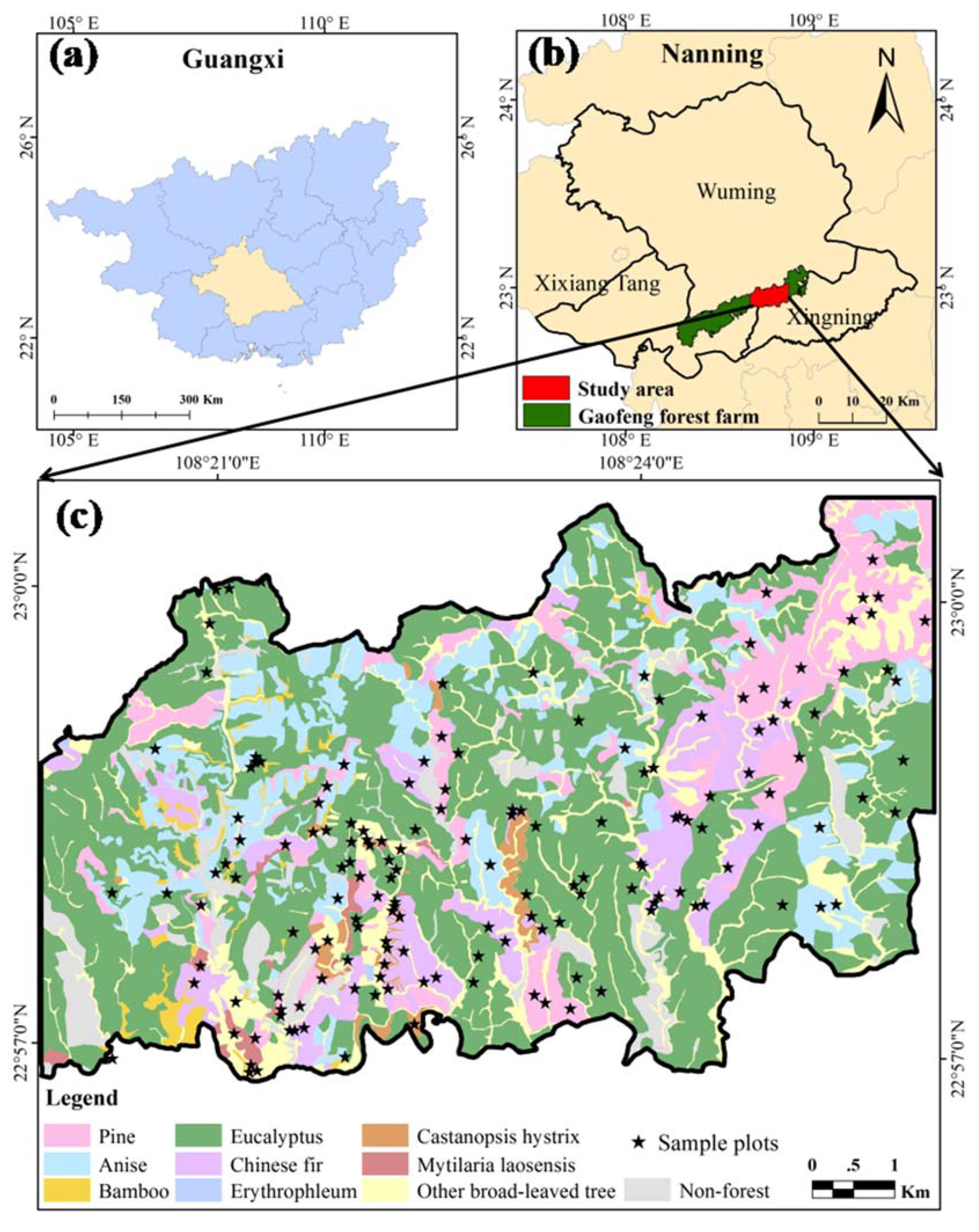
The study area is located in Jiepai and Dongsheng within the Gaofeng Forest Farm (Figure 2) with an area of 56.3 km2. According to the lidar-derived digital elevation model (DEM) data, the elevation ranges from 73.4 to 463.6 m and the slope ranges from 0° to 69.7° with the majority of slopes between 20° and 35°. According to the forest inventory data of 2016, the main forest types in the area are eucalyptus, Chinese fir, Masson pine, and star anise. In particular, eucalyptus plantations have expanded rapidly since 2002 because of their important economic value for local government and farmers.
2.2. Field Survey and Biomass Calculation at the Plot Level
A field survey of the Gaofeng Forest Farm was conducted in January and February 2018, the same period as the airborne lidar data collection. Using the forest distribution mapped in 2016, sample plots were allocated using a stratification sampling approach according to areas of specific forest types and their age groups. From our study area which consisted of two subfarms (Jiepai and Dongsheng) within this forest farm (see Figure 2), a total of 71 sample plots were allocated. After carefully examining the location and measurement quality, 11 samples were eliminated because the forests, mainly eucalyptus due to its short harvest rotation, had been clear cut. Thus, 60 sample plots, including 37 eucalyptus, 17 coniferous (mainly Chinese fir), and 6 other broadleaf forests, were used. Each sample plot contained the same forest type without a mix of different land covers, and therefore each sample represented a specific forest type. Different plot sizes of 20 x 20 m and 25 x 25 m were used during the field survey based on forest ages and working loads. The coordinates of each sample plot were recorded. Tree species, height, crown diameter and height, and DBH for each individual tree within a sample plot were recorded and measured. The allometric models for major tree species in Guangxi (eucalyptus, Masson pine, Chinese fir, hardwood broadleaf species, and softwood broadleaf species) [52] were used to calculate individual tree AGB. The AGB of a sample plot was the total of individual tree AGBs within the sample plot. Then, the AGB, at the plot level, was converted to AGB at one hectare (Mg/ha). The allometric model can be expressed as
where W is the AGB of an individual tree (kg); D is DBH (cm); H is tree height (m); and c1, c2, and c3 are coefficients for a specific tree species. Table 1 lists the coefficients used in Equation (1) for different tree species [52].
Our collaborator conducted the fieldwork from October to November 2017 and provided the coordinates and forest volume, but not the AGB, for each sample plot. A total of 98 sample plots (plot size of 30 x 30 m) were collected. By examining these sample plots and our lidar data, three plots were excluded because they were outside our study area. Thus, the 95 sample plots included 18 eucalyptus, 20 Chinese fir, 29 Masson pine, and 28 other broadleaf forests.
In order to use the field survey data, it was necessary to convert forest volume to AGB for each sample plot. Thus, based on the sample plots from 2018, we used the same approach to calculate tree volume using the DBH and height for each tree species, and then calculated forest volume for each plot by taking the total volume of individual trees within the same plot. On the basis of the relationship between the AGB and the forest volume at plot level, a LR equation for each forest type was developed, in which AGB is a dependent variable and forest volume is an independent variable. The results showed that the R2 (coefficient of determination) and relative root mean square error (RMSEr) were, respectively, 0.99 and 3.2% for eucalyptus, 0.83 and 7.9% for coniferous species, and 0.92 and 8.4% for other broadleaf species. Thus, all sample plots collected in 2017 were converted from volume to AGB.
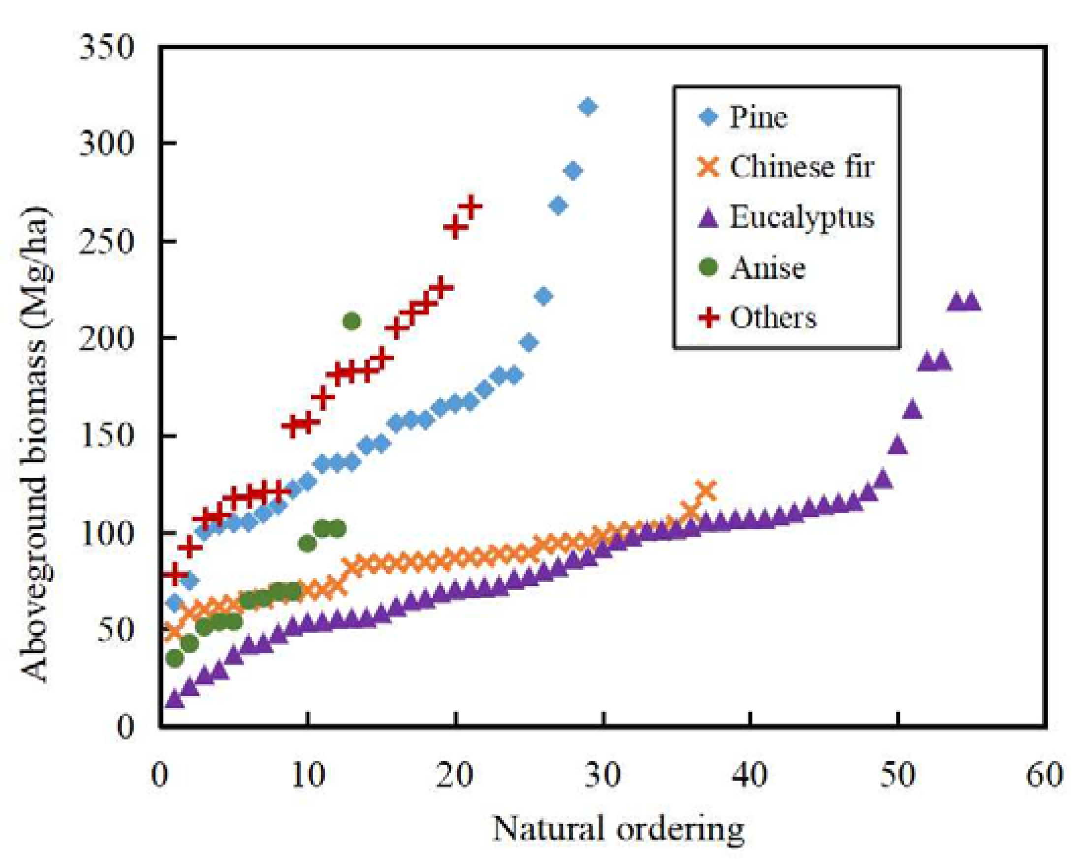
Because the gap between the two surveys was only two months, we combined the surveys into one dataset to enlarge our sample size. Table 2 summarizes the statistics of samples, showing that the AGB values for all forest types span from 14.7 to 318.6 t/ha with a coefficient of variation (CV) of 0.51. The detailed AGB distribution of different forest types is illustrated in Figure 3. Eucalyptus and Chinese fir have the most sample plots; however, the AGB values are very concentrated within the range of 50 to 00 t/ha, in particular, Chinese fir has the smallest AGB range and standard deviation. Overall, Chinese fir has the smallest CV value of 0.19 and star anise has the largest CV value of 0.57.
2.3. Update of Forest Distribution Map
In order to develop AGB estimation models for stratified forest types, an accurate forest distribution map is needed. In this study, the Gaofeng Forest Farm provided a forest distribution map that had been developed in 2016 based on a field survey. According to this map and our research objective, a classification system of 10 land covers was determined as follows: Chinese fir, Masson pine, eucalyptus, star anise, Mytilaria laosensis, Castanopsis hystrix, Erythrophleum fordii, other broadleaf tree species, bamboo, and non-forest types (e.g., shrubs, impervious surface, water, and bare soil). The forest distribution map with digital vector format was superimposed on the high-resolution aerial photograph (0.2 × 0.2 m) taken at the same time as the airborne Lidar data were gathered, in January 2018. The analyst carefully checked each forest patch by visual interpretation and comparison between the forest distribution map and aerial photograph. If the boundary of a forest patch had changed, a new boundary was drawn, and the corresponding forest type was updated. This visual interpretation ensured high accuracy in updating the forest distribution map and was effective when there was little change in the land covers. Figure 2c illustrates the spatial distribution of the updated forest types that was used for AGB estimation in this research.
2.4. Design of Stratification Scenarios
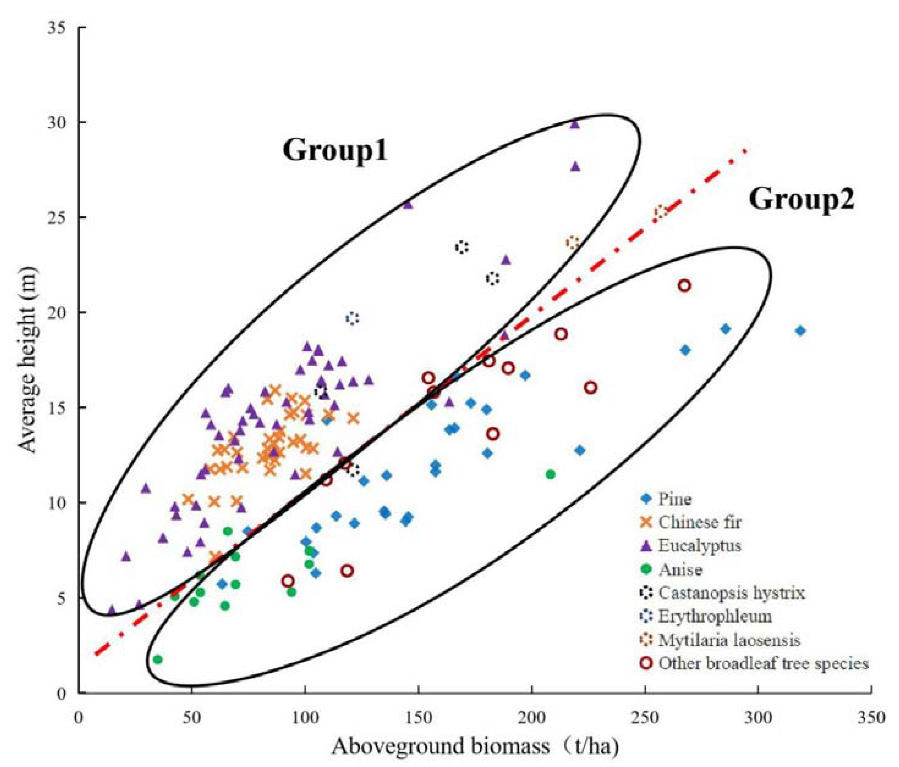
Most previous studies on forest AGB estimation have not differentiated forest types in developing estimation models, ignoring the variations in the relationships between AGB and canopy height among forest types or tree species, largely due to the limitation in collecting a sufficient number of sample plots [50]. A few studies have proven that separately developing AGB estimation models based on stratified forest types improved predictions [24,50]. However, how to stratify forest types, that is, what criteria can be based on and how many strata are optimal, remains unclear. Thus, we designed different stratification scenarios (Table 3) to examine how they affect the estimation results. The first stratification approach was species based, and forest samples were grouped into two broad groups (coniferous and broadleaf) and five finer groups (Masson pine, Chinese fir, eucalyptus, star anise, and other broadleaf species). The second stratification approach was based on the relationships between canopy height and forest AGB (Figure 4). The red dashed line in Figure 4 divides all forest samples into two groups. Group 1 mainly consisted of eucalyptus, Chinese fir, Castanopsis hystrix, Erythrophleum fordii, and Mytilaria laosensis, and Group 2 mainly consisted of Masson pine, star anise, and other broadleaf species. Although both Chinese fir and Masson pine are coniferous, the relationships between canopy height and AGB were significantly different; in contrast, Chinese fir and eucalyptus showed similar trends in their relationships between canopy height and AGB. As a comparison, all forest types were used as one population for the AGB modeling.
2.5. Collection and Processing of Airborne Lidar Data
The airborne lidar data for the Gaofeng Forest Farm were acquired on 13 and 30 January 2018, using a Riegl LMS-Q680i lidar scanner mounted on the LiCHyAOS system. The specifications of the lidar sensor are shown in Table 4. The lidar data provider preprocessed the raw data and labeled each echo signal as ground return or nonground return before delivering to the end users. The nonground return points were used to generate the digital surface model (DSM) and the ground points were used for the digital elevation model (DEM) at a pixel size of 1 x 1 m using a triangulated irregular network (TIN) interpolation algorithm. The canopy height model (CHM) data were produced from the differences between the DSM and DEM. This initial CHM recorded the maximum object height within a pixel. It could have been contaminated by artificial objects such as power poles, power lines, or towers. Thus, pixels with values greater than 50 m were checked on the aerial photograph with spatial resolution of 0.2 m. If these pixels were found to have abnormal values, they were replaced with the mean value using a mean filter operation.
A number of predictive variables for the AGB estimation were extracted from the CHM data with a uniform window size of 20 × 20 m. The central point of each plot was used to link the sample plot to the CHM image to extract variables according to the window size. The commonly used statistical metrics such as mean, quadratic mean, and height percentiles (10 to 100) [28,33,36] were extracted. Meanwhile, we also explored texture measures using the gray level co-occurrence matrix (GLCM) within the size of the sample plot (20 × 20 m) to extract textural images from the CHM data. The texture measures included correlation, contrast, dissimilarity, entropy, homogeneity, second-order moment, and variance [53,54]. These metrics and the corresponding forest AGB of sample plots were exported to SPSS for further analysis.
2.6. Development of Biomass Estimation Models
Many previous studies have indicated that when lidar data are used for forest biomass estimation, linear regression (LR) is one of the most widely used parametric modeling approaches [34,36,55]. The LR approach assumes a linear relationship between the dependent variable (forest AGB here) and predictive variables (lidar-derived variables here). Because a large number of potential variables can be used for AGB modeling, it is necessary to identify key variables that largely explain the variance of the dependent variable [1]. One common approach to identify key variables is stepwise regression analysis. Stepwise regression analysis is able to determine inclusion or exclusion of variables based on the test statistics of estimated coefficients via a series of F-tests or T-tests. It builds a model by successively adding or removing one variable at a time [30]. The key variables that were finally selected were used to develop the AGB model using the LR approach. In order to understand the importance of different variables in the developed LR model for AGB estimation, standard coefficients (beta) were used to show which variables were more important than others; that is, the higher beta value (absolute value) indicated its higher importance in the LR model.
Considering the potentially nonlinear relationships between AGB and lidar-derived metrics, RF is an alternative. Approach for identifying key variables for AGB modeling. RF is an improved decision tree-based algorithm that uses the bagging and boosting theory. Many trees are produced from the random selection of variables and samples, and thus the final result is based on the ensemble of the individual trees [31]. Compared with the traditional decision tree algorithm, the RF algorithm has some advantages such as insensitivity to noisy data in training datasets, using discrete or continuous datasets, and dealing with large datasets [56]. Many previous studies have indicated that the RF algorithm provides better classification results or estimations than the decision tree algorithm; therefore, the RF algorithm has been widely applied to quantitative analysis such as land-cover classification and AGB estimation [9,15,57,58]. We used the RF algorithm to identify potential key variables, then correlation analysis was used to examine the relationships between these potential variables. For a variable having high correlation with other variables while having less importance in the ranking, this variable was removed, and the RF algorithm was re-run. This procedure was repeated until the minimum number of variables was obtained without reducing the AGB modeling performance. The selected key variables were finally used to develop the AGB estimation model using a RF approach.
2.7. Evaluation of Biomass Modeling Results and Application of the Developed Models to Entire Study Area
An evaluation of the modeling performances is often required to understand whether the developed model is suitable for the AGB estimation for the entire study area [10]. Different quantitative measures such as R2, RMSE, mean absolute error, system error, Akaike’s information criterion, and Bayesian information criterion can be used [59,60]. In addition to the traditional accuracy assessment measures, Valbuena et al. [61] indicated the necessity to also conduct an accuracy assessment of the AGB estimates through hypothesis testing and overfitting evaluation. Considering the validation data used, two methods are often used for the evaluation of AGB estimates [18]. The first approach uses independent testing samples that are different from training samples. The second approach is cross-validation, which is one of the most widely used tools for accuracy assessment, especially with a small number of samples [62]. Cross-validation randomly partitions the samples into several disjointed subsets of approximately equal size (m-fold); each subset is used as testing data, and the remaining subsets are used as training data. The model generated from the training subsets is applied to the testing data to estimate the expected discrepancy. This process is repeated until all possible subsets of samples have been used once; then, the estimation accuracies across all blinded tests are combined to give an overall performance estimate [24,63]. In this study, we used leave-one-out cross-validation for model development and accuracy assessment. One sample was left out and the remaining samples were used to construct the LR model or RF model. This process was repeated, removing each sample in the sample data one by one. Therefore, for each validation, almost all samples were used as training data, which produced reliable prediction, avoiding the impact from random factors. The accuracy of models was assessed by R2, RMSE, and RMSEr [64]. By comparing the performances of those models developed using LR and RF algorithms under four stratification scenarios, the best model for the corresponding scenario was selected and applied to predict the forest AGB of the entire study area. In addition to the overall accuracy assessment, R2, RMSE, and RMSEr were calculated for evaluation of the modeling results according to individual forest types (i.e., Masson pine, Chinese fir, eucalyptus, star anise, and others) and AGB ranges (i.e., <50, 50–100, 100–150, 150–200, 200–250, and >250 Mg/ha). On the basis of these evaluation results, the best modeling results for the forest types were combined to generate a new AGB map with the highest estimation accuracy.
3. Results
3.1. Comparative Analysis of Biomass Estimation Models
A comparative analysis of the AGB models (see Table 5) indicates that in the LR-based AGB models, (1) HME is often selected for the AGB estimation models and has a higher beta value than other selected variables, implying that it is a more important variable and (2) for individual tree species such as Chinese fir, eucalyptus, and star anise with relatively simple stand structures, only one variable is selected, but for the complex forest types such as coniferous or broadleaf forests, more variables related to forest stand structure, in addition to HME, are needed. Table 5 also shows that overall the RF-based models have higher R2 values and require more variables than LR-based models. The selected variables vary in different stratification scenarios. Even in the same scenario of SBFT5, the selected variables for each forest type vary, implying the importance of identifying suitable variables for specific tree species.
3.2. Comparative Analysis of Biomass Estimation Results
3.2.1. Overall Evaluation of Biomass Modeling Results
The AGB estimation results based on different scenarios (Table 6) indicate that the LR model has slightly poorer performance than the RF model based on NonS and SBFT2, but the inverse based on the SBFT5 and SBFSS scenarios. Overall, the LR model based on the SBFT5 scenario performs the best, with R2 of 0.8 and RMSE of 25.36 Mg/ha; in contrast, the LR model based on the SBFT2 scenario has the poorest performance, with R2 of 0.43 and RMSE of 44.07 Mg/ha, implying the importance of detailed stratification of forest types. The results in Table 6 also indicate that improper stratification, i.e., coniferous and broadleaf forest (SBFT2), cannot improve the AGB estimation, but a good stratification, such as the SBFSS scenario here, can significantly improve the AGB estimation, that is, R2 increased from 0.43 (based on SBFT2) to 0.78 (based on SBFSS) and RMSE decreased from 44.07 Mg/ha to 26.0 Mg/ha. On the one hand, more detailed stratification (SBFT5) performs similarly to the SBFSS scenario when the LR model is used. On the other hand, when the RF model was used, the SBFSS scenario provided the best AGB modeling results. This situation implies that very detailed stratification of forest types is not needed. The finding is valuable for guiding the collection of sample plots and the possibility of using a small number of them for the AGB estimation in some forest types.
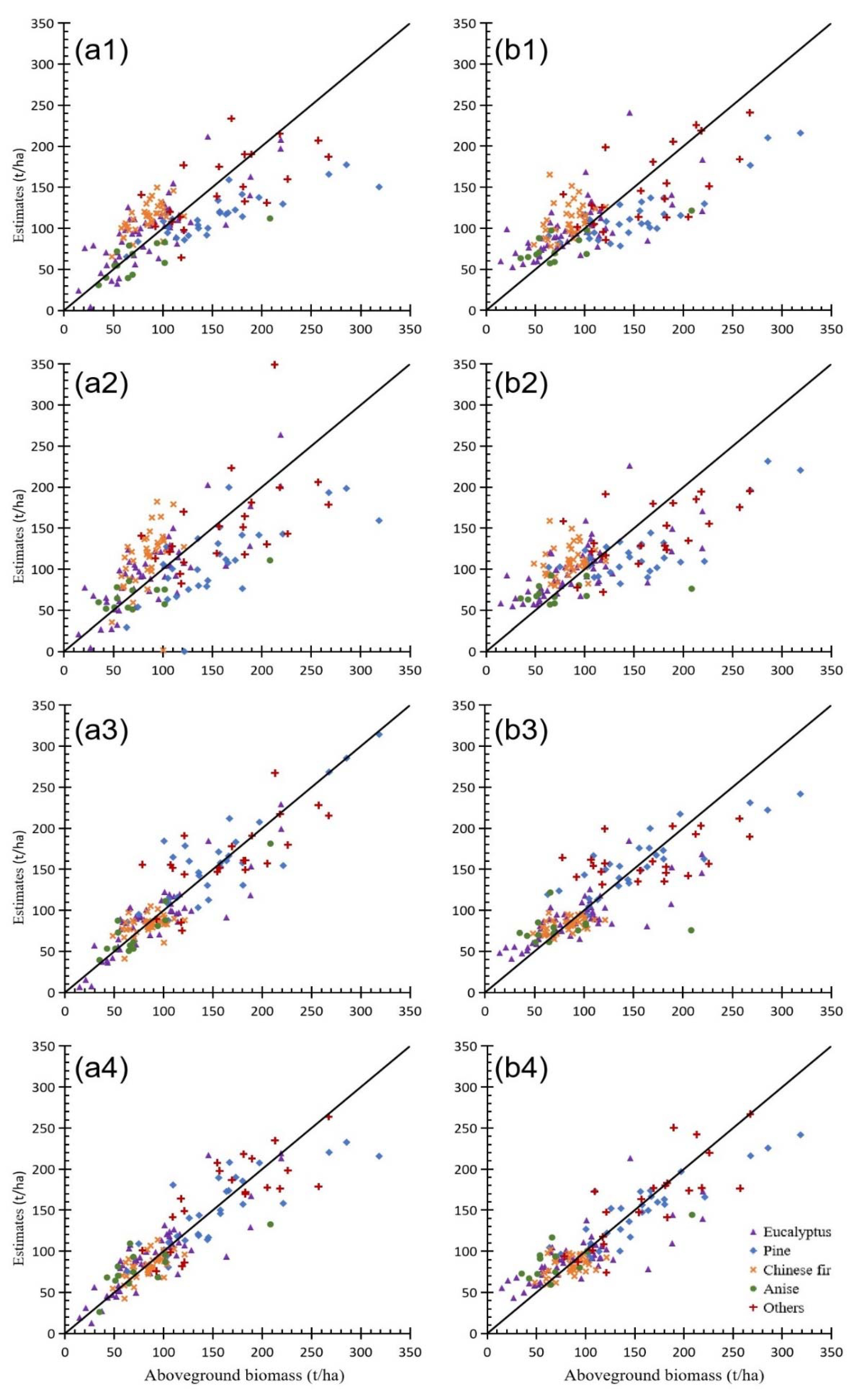
A comparative analysis of the relationships between AGB estimates and reference data (Figure 5) indicates that (1) both the LR and RF models based on the SBFT5 or SBFSS scenarios (Figure 5a3,a4,b3,b4) perform better than those based on NonS or SBFT2 (Figure 5a1,a2,b1,b2); (2) compared to the the LR modeling results, the RF modeling results have a common problem, that is, when AGB is less than ~50 Mg/ha, AGB was overestimated; (3) except for the LR modeling result based on the SBFT5 scenario, underestimation is obvious, especially when AGB is greater than 220 Mg/ha. Figure 5 also shows that the LR model based on the SBFSS scenario (Figure 5a4) is the best when AGB is less than ~120 Mg/ha, and the LR model based on the SBFT5 scenario (Figure 5a3) is the best when AGB is greater than ~270 Mg/ha.
3.2.2. Evaluation of Biomass Estimation Results According to Individual Forest Type
The evaluation results according to different forest types (Table 7) indicate that the modeling based on the SBFT5 or SBFSS scenarios using the LR and RF approaches performed much better than modeling based on the NonS and SBFT2 scenarios. The RMSEr values are 19.7% to 21.7% for Masson pine and 15.9% to 18.9% for Chinese fir based on the SBFT5 and SBFSS scenarios, respectively, as compared with 32.6% to 39.5% and 39.2% to 52.6% based on the NonS and SBFT2 scenarios, respectively. Overall, the LR model based on the SBFT5 scenario provided the best results for eucalyptus and star anise, while the LR model based on the SBFSS scenario provided the best results for Chinese fir (RMSEr ~16%), and the RF model based on the SBFSS scenario provided the best result for “others” class (other broadleaf species). This evaluation result implies the importance of proper stratification for improving AGB estimation. For example, if AGB models were separately developed for Masson pine and Chinese fir, the RMSE for Masson pine could be reduced from 55.7 Mg/ha (NonS) and 61.4 Mg/ha (SBFT2) to 31.2 Mg/ha (SBFT5), and for Chinese fir from 32.7 and 43.8 Mg/ha to 15.6 Mg/ha, respectively. Table 7 also indicates that for different forest types, the best modeling approach varies, for example, for the SBFT5 scenario, the RF model provided slightly better modeling results for Masson pine and Chinese fir than for LR, whereas the LR model provided better results for eucalyptus, star anise, and “others.” Another finding in Table 7 is that star anise provides much better estimation using the LR model based on the SBFT5 scenario, implying that when the number of sample plots is not large, the LR model is more reliable than the RF model. However, for a complex forest type, the “others” class, in this study, with a limited number of sample plots, the SBFSS scenario with an RF algorithm provides the best estimation, implying the advantage of using the SBFSS scenario.
3.2.3. Evaluation of Biomass Estimation Results According to Biomass Ranges
The evaluation results according to the AGB ranges (Table 8) indicates that proper stratification of forest types (SBFT5 and SBFSS scenarios) considerably improves the AGB estimation for each AGB range, especially when the AGB is low (e.g., less than 50 Mg/ha) or high (e.g., greater than 200 Mg/ha). When the AGB is less than 50 Mg/ha, the LR model based on the SBFT5 scenario provides the best estimation, followed by the SBFSS scenario with RMSE less than 13.5 Mg/ha. When the AGB is 50 to 150 Mg/ha, the LR model based on the SBFSS scenario has the best estimation with RMSE 17.1 to 24.2 Mg/ha, and when the AGB is greater than 150 Mg/ha, the SBFT5 scenario has the best estimation with RMSE 26.7 to 40.5 Mg/ha. Comparing Table 8 with Figure 5, we find that stratification of forest types using the SBFT5 and SBFSS scenarios considerably reduced the underestimation problem. In particular, when the AGB was greater than 200 Mg/ha, the SBFT5 scenario greatly reduced the underestimation problem.
As shown in Table 6, the SBFT5 and SBFSS scenarios have much better modeling estimates than the NonS and SBFT2 scenarios, no matter which algorithm, LR or RF, is used. However, considering different AGB ranges, the LR and RF algorithms perform differently. For instance, based on the SBFT5 scenario, the LR algorithm performs much better than the RF algorithm when the AGB is less than 50 Mg/ha or more than 200 Mg/ha and slightly better than the RF algorithm when the AGB is 50 to 100 or 150 to 200 Mg/ha, but the LR algorithm performs poorly as compared with the RF algorithm when the AGB is 100 to 150 Mg/ha (RMSEr is 26.1% for the LR algorithm and 23.6% for the RF algorithm). This situation implies that for a finer stratification scenario, the overfitting problem with the RF algorithm is obvious, resulting in an overestimation and underestimation problem, especially when the number of samples is relatively small. For the SBFSS scenario, the LR algorithm performs much better than the RF algorithm when the AGB is less than 50 Mg/ha (RMSEr is 38.1% for the LR algorithm and 80.0% for the RF algorithm) and slightly better than the RF algorithm when the AGB is 50 to 200 Mg/ha, (difference within 0.3% to 2.0% between the LR and RF algorithm results), but the LR algorithm performs poorly as compared with the RF algorithm when the AGB is greater than 200 Mg/ha (difference within 1.8% to 3.4% between the LR and RF results). This situation implies that when the AGB is more than 200 Mg/ha, the AGB and canopy height cannot meet the linear assumption, because the SBFSS scenario is grouped based on the relationship between the canopy height and the AGB (see Figure 4). In this case, the RF algorithm handles the nonlinear relationship better than that of the LR algorithm. The results in Table 8 imply that it is necessary to select different algorithms to develop specific AGB estimation models by taking the stratification and AGB ranges into account.
3.3. Comparative Analysis of Biomass Spatial Distributions
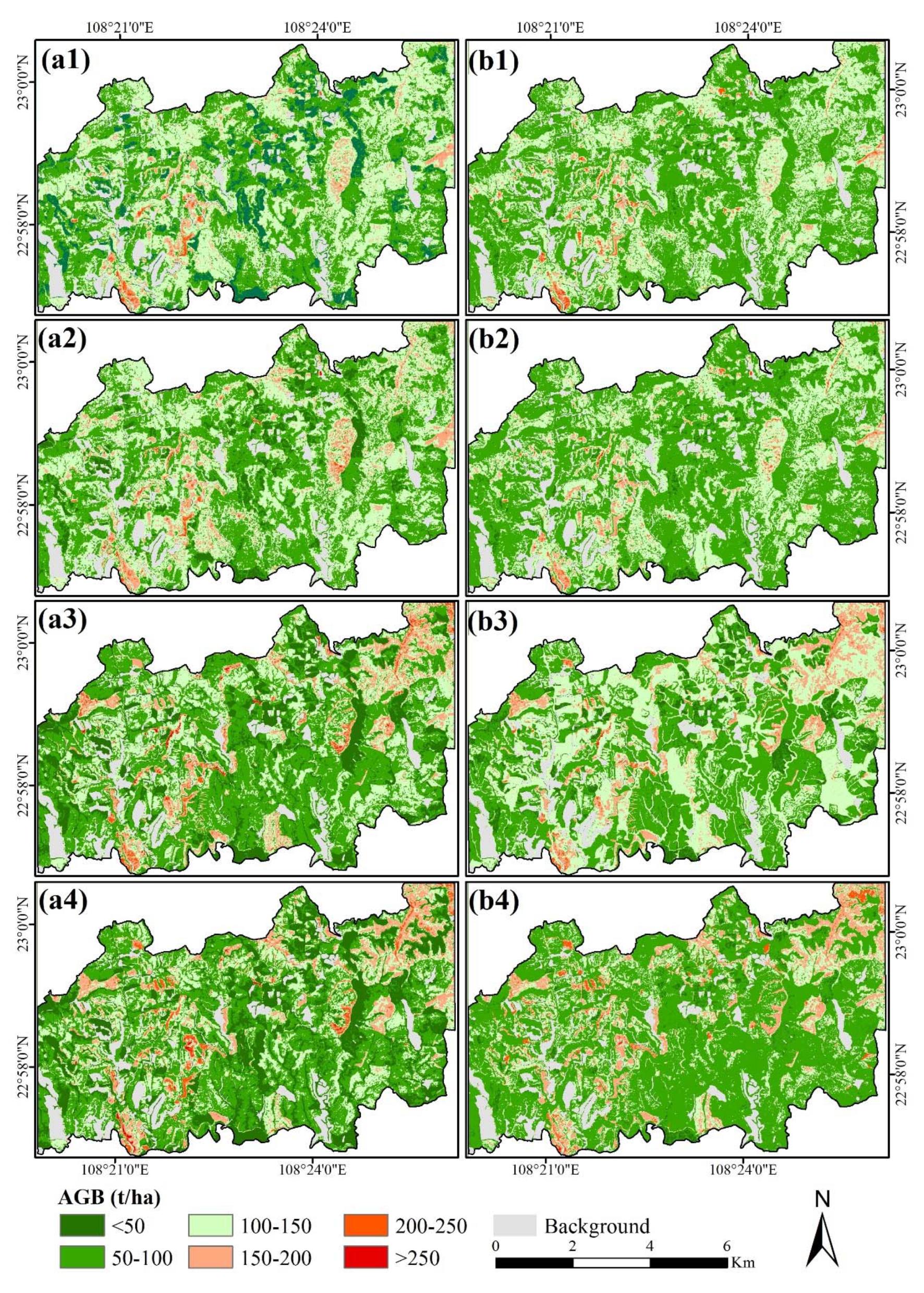
The spatial distributions of AGB predictions based on the LR and RF models under different scenarios (Figure 6) indicate that most of the study area has 50 to 200 Mg/ha of AGB, and a few areas have less than 50 Mg/ha or greater than 200 Mg/ha. The spatial distribution indicates that the LR model prediction results have many more pixels with less than 50 Mg/ha or higher than 200 Mg/ha as compared with the RF model prediction results, implying the inability of the RF model to predict very low or very high AGB amounts.
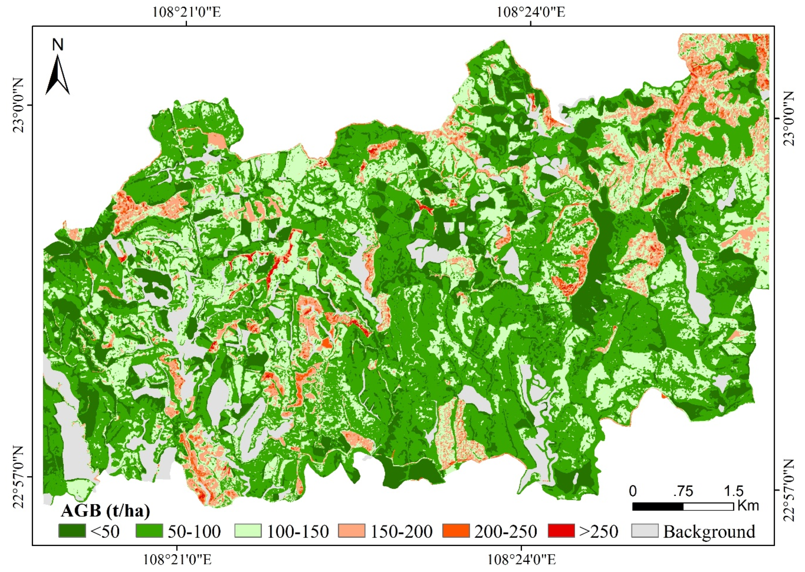
Table 7 indicates that different forest types require specific stratification and modeling approaches; thus, the best modeling result for each forest type provides the best AGB prediction map (Figure 7). A comparison of the spatial patterns in Figure 6 and Figure 7 shows that the number of pixels with very low (less than 50 Mg/ha) or very high (greater than 250 Mg/ha) values is obviously large in Figure 7, implying much improved modeling results.
4. Discussion
4.1. Impact of Stratification on Aboveground Biomass Modeling
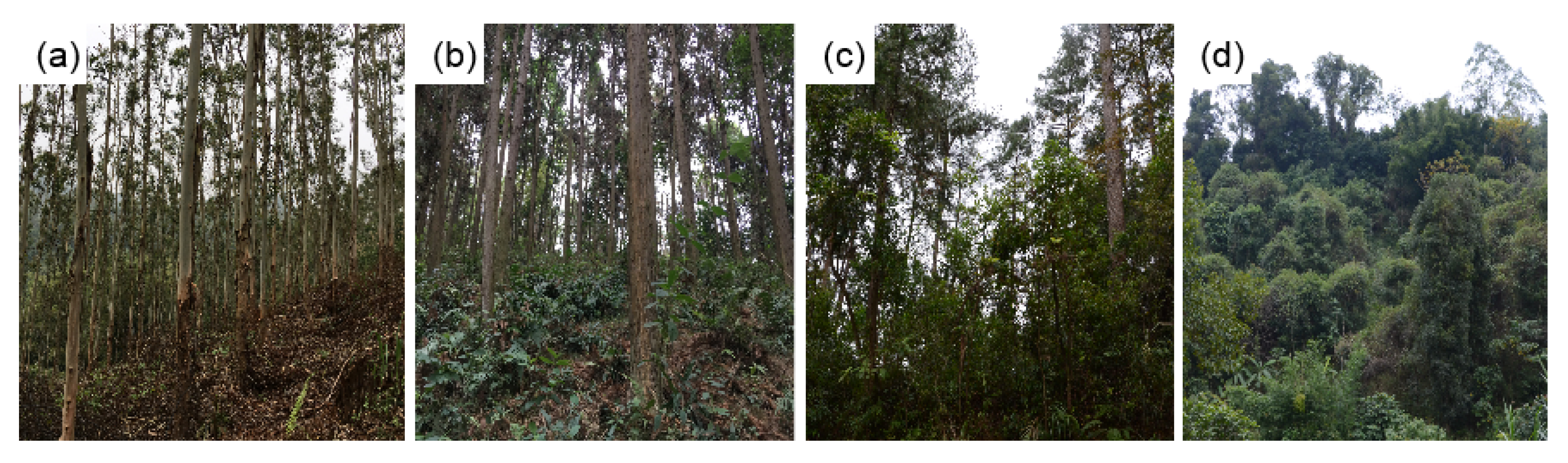
Forest AGB is related to tree species composition and tree density in a unit, in addition to wood density, DBH, and tree height of individual tree species. For optical sensor data, data saturation is a big problem that results in poor AGB estimation because optical sensor data mainly capture land surface features without vertical forest stand information [20]. Lidar data measure tree or canopy height, and thus are regarded as the most accurate data source for AGB estimation because of the strong correlation between AGB and canopy or tree height [25]. Some previous studies using Landsat data have proven the effectiveness of stratification of forest types for improving AGB estimation [9,20]. However, airborne lidar data are only available at experimental sites with a limited area; thus, sample plots are often limited [24,65] and non-stratification is common in most previous studies. Cao et al. [27] confirmed that stratification of forest types reduced the overall RMSEr from 22.7% to 15.84% for coniferous forest type, 15.41% for broadleaf forest type, and 18.33% for mixed forest type. Our research indicates that proper stratification of forest types considerably improved the AGB modeling performance, but improper stratification reduced performance. For example, although Masson pine and Chinese fir belong to coniferous forests, their crown size and shape and their relationships between AGB and canopy height are different. This research shows that the AGB modeling based on coniferous forest (e.g., a combination of Masson pine and Chinese fir) reduced modeling performance, while modeling based on individual tree species considerably improved it. As indicated in Table 7, the RMSEr values for Masson pine and Chinese fir using the LR model based on the SBFT2 scenario increased by 3.7% and 13.4%, respectively as compared with those based on the NonS scenario, while they reduced by 24.5% and 17.1% based on the SBFT5 scenario. The RF-based model based on the NonS and SBFT2 scenarios provided similar modeling performances for Masson pine and Chinese fir, but based on the SBFT5 scenario, the RMSEr values decreased by 13.3% and 22.8%, respectively for those species. This result differs from some previous studies [27,29,39]. The possible reason is that Chinese fir is often in a pure plantation with homogenous stand structure and age, while the stand structure of Masson pine is often complex and mixed with some broadleaf tree species in the canopy and with shrubs and grass under canopy, as shown in Figure 8.
Our research indicates that the SBFT5 scenario provides the best modeling performance but requires a large number of sample plots for each tree species. This is often a challenge for most studies, considering the cost and labor of sample data collection. Another challenge in using the SBFT5 scenario is the detailed classification of tree species, which is often difficult because of the similar spectral signatures of different broadleaf tree species. However, many tree species have similar relationships between tree height and AGB, and we can combine them into one group. This implies that we are able to collect fewer sample plots for AGB modeling and still produce similar modeling results, as shown in Table 6, that is, R2 and RMSE are similar for the SBFSS and SBFT5 scenarios using the LR model, and slightly better when using the RF model. Another advantage is that for some forest types with limited area, the SBFSS scenario can provide modeling results, but the SBFT5 scenario cannot. The challenge of using the SBFSS scenario is to clearly understand the relationships between tree height and AGB for different tree species, and thus expert knowledge is essential for determining the grouping if sufficient sample plots are not available.
4.2. Impacts of Sample Sizes on Aboveground Biomass Modeling
The collection of a sufficient number of sample plots is one of the most important steps in AGB estimation [10]. However, in reality, the collection of sample plots is greatly hindered by cost and labor intensity, which seriously affect modeling performance, that is, they affect the determination of stratification of forest types, selection of modeling variables and algorithms, and the evaluation of modeling results. For example, with the numbers of samples for Masson pine, Chinese fir, and eucalyptus at 29, 37, and 55, we developed the LR model for each species. As shown in Table 7, the RMSEr values for Masson pine, Chinese fir, and eucalyptus were, respectively, reduced from 35.8%, 39.2%, and 31.3% based on the NonS, to 20.0%, 18.7%, and 24.8% based on the SBFT5 scenario. However, if the AGB range of a sample plot is not representative, the selection of modeling algorithms is seriously affected. For instance, star anise has only 13 sample plots and only one with the AGB greater than 200 Mg/ha; as a result, the RF model’s RMSEr is 56.8% as compared with 21.0% in the LR model. A similar situation occurs for eucalyptus, that is, of 55 samples, only five have AGB greater than 150 Mg/ha. Thus, the RF-based models performed poorly as compared with the LR-based models (Table 7). This implies that collection of a sufficient number of sample plots with good representation of different AGB ranges is critical for AGB estimation.
4.3. Impacts of Forest Types on Selection of Modeling Variables and Algorithms
There is no universal conclusion about what variables should be used for AGB modeling, because they depend on forest types, complexity of the landscape under investigation, individual tree species, and the algorithms [9,20]. Our research confirms that different variables must be used for specific stratification scenarios and modeling methods. This implies that developing an optimal model should take into account the specific forest types and their complexities of forest stand structure, as well as the modeling algorithm. As shown in Table 5, for a forest composed of a single tree species, such as Chinese fir, eucalyptus, or star anise, where all trees are the same age, only one variable was selected for the LR model, whereas two or more variables were selected for complex forest types such as Masson pine (pine dominant in top canopy and broadleaf tree species dominant under canopy), and “others” (composition of different tree species). For the RF models, more variables were selected than for the LR models. However, using more variables does not guarantee better prediction results because of the overfitting problem in the RF algorithm. As shown in Figure 5, the RF algorithm did not have a good extrapolation ability, especially for the forest types with a limited number of sample plots with low or high AGB ranges. This research shows the importance of selecting proper variables by taking into account the different characteristics of forest types.
The complexity of a forest stand structure also affects the selection of modeling algorithms. As shown in Table 7, the RF algorithm performs better than the LR algorithm in NonS and SBFT2 scenarios, while the inverse occurs in SBFT5 and SBFSS scenarios, implying that for complex forest types, a machine learning algorithm is more suitable than the LR algorithm. This could be due to the fact that the LR algorithm cannot effectively delineate the nonlinear and complex relationships between the forest attributes and the AGB [32,39]. For a forest type with relatively simple stand structure, such as eucalyptus, the LR algorithm performs better, especially for extrapolation when a limited number of samples for high and low AGB samples are used, as shown in Figure 5. This research implies that when the number of sample plots is insufficient, the LR approach is better than the RF approach, and that a sufficient number of samples with relatively low and high AGB must be collected for the RF approach to reduce the over- and underestimation problems [20,24].
4.4. Impacts of Amounts of Forest Aboveground Biomass on Modeling Results
How different amounts of forest AGB affect modeling results has not been extensively explored, especially for the Lidar-based AGB estimation. Limited research has examined AGB under- and overestimation using Landsat and ALOS PALSAR data in a subtropical region [9,20,22]. The overestimation in optical or radar data mainly occurs in forest sites with relatively low AGB such as less than 50 Mg/ha, because of the complex composition of land-cover components in one pixel (shrub, grass, or bare soil in addition to tree density), whereas underestimation occurs in dense forests with high AGB, such as more than 150 Mg/ha, due to the data saturation problem [20]. Compared to optical or radar data that mainly capture canopy features without much information on forest height, Lidar data obtain canopy height features that are highly related to AGB, resulting in high estimation accuracy, as shown in this research (Table 8), especially when finer stratification is used. In the SBFSS scenario, when AGB is higher than 200 Mg/ha, the RF approach provides better modeling performance than the LR approach, implying that when AGB is relatively high, AGB may be nonlinearly related to CHM-derived variables. This research also implies that stratification based on forest types and AGB ranges provides better modeling results. This should be explored in the future if a large number of sample plots are available.
5. Conclusions
This research explored lidar-based AGB modeling in a subtropical forest ecosystem using LR and RF approaches based on different stratifications of forest types. Through comparative analysis of modeling results, this research provided some new insights on how to implement stratification of forest types and how to identify suitable variables for AGB modeling based on different forest types. Specifically, we state the following conclusions:
- (1)
- The complex composition and rich tree species in a subtropical ecosystem make AGB estimation a challenge, resulting in high uncertainty in AGB modeling, especially when the AGB is relatively low (e.g., <50 Mg/ha) or high (e.g., >200 Mg/ha). Proper stratification of forest types for AGB modeling is an effective approach to improve AGB estimation.
- (2)
- AGB modeling based on specific forest types provides the best AGB modeling results but requires a large number of sample plots for each forest type, resulting in a challenge in sample data collection and in classification of detailed forest types. Stratification based on the relationship between canopy height and AGB (SBFSS in this study area) solves this problem and provides similar modeling performance.
- (3)
- Selection of modeling variables depends on the complexity of the forest types or forest stand structures. More variables are often required for the NonS and SBFT2 scenarios or complex forest types (Masson pine) than for detailed stratification with individual forest types.
- (4)
- The LR model is suitable for AGB modeling for the forest types with relatively simple forest stand structure such as Chinese fir, eucalyptus, and star anise, while the RF model is suitable for complex forest types such as broad groups, that is, coniferous and broadleaf forest types.
- (5)
- Stratification based on the relationship between canopy height and AGB (the SBFSS scenario) is recommended for AGB modeling, considering performance and requirement of sample sizes.
Author Contributions
Conceptualization, D.L. and E.C.; methodology, D.L., and X.J.; software, X.J.; validation, X.J. and G.L.; formal analysis, X.J. and G.L.; investigation, X.J., G.L., and D.L.; resources, X.J.; data curation, X.J. and G.L.; writing—original draft, G.L., D.L., and X.J.; writing—review and editing, D.L., G.L., X.W., and E.C.; visualization, D.L.; supervision, D.L. and X.W.; project administration, D.L. and E.C.; funding acquisition, D.L. and E.C. All authors have read and agreed to the published version of the manuscript.
Funding
This study was financially supported by the National Key R&D Program of China project “Research of Key Technologies for Monitoring Forest Plantation Resources” (2017YFD0600900) and by the National Natural Science Foundation of China (grant #41571411).
Acknowledgments
The authors would like to thank Lei Zhao, Longwei Li, Yaoliang Chen, Xiaozhi Yu, and Shuai Zhao for their help in the fieldwork.
Conflicts of Interest
The authors declare no conflicts of interest.
References
- Yu, X.; Ge, H.; Lu, D.; Zhang, M.; Lai, Z.; Yao, R. Comparative Study on Variable Selection Approaches in Establishment of Remote Sensing Model for Forest Biomass Estimation. Remote Sens. 2019, 11, 1437. [Google Scholar] [CrossRef] [Green Version]
- Piao, S.; Fang, J.; Ciais, P.; Peylin, P.; Huang, Y.; Sitch, S.; Wang, T. The carbon balance of terrestrial ecosystems in China. Nature 2009, 458, 1009–1013. [Google Scholar] [CrossRef] [PubMed]
- Tan, Z.-H.; Zhang, Y.-P.; Schaefer, D.; Yu, G.; Liang, N.; Song, Q. An old-growth subtropical Asian evergreen forest as a large carbon sink. Atmos. Environ. 2011, 45, 1548–1554. [Google Scholar] [CrossRef]
- Shen, W.; Xu, T.; Li, M. Spatio-temporal changes in forest fragmentation, disturbance patterns over the three giant forested regions of China. J. Nanjing For. Univ. 2013, 37, 75–79. [Google Scholar]
- Liu, S.; Wei, X.; Li, D.; Lu, D. Examining Forest Disturbance and Recovery in the Subtropical Forest Region of Zhejiang Province Using Landsat Time-Series Data. Remote Sens. 2017, 9, 479. [Google Scholar] [CrossRef] [Green Version]
- Wen, X.-F.; Wang, H.-M.; Wang, J.-L.; Yu, G.; Sun, X.-M. Ecosystem carbon exchanges of a subtropical evergreen coniferous plantation subjected to seasonal drought, 2003–2007. Biogeosciences 2010, 7, 357–369. [Google Scholar] [CrossRef] [Green Version]
- Zhang, W.J.; Wang, H.-M.; Yang, F.-T.; Yi, Y.-H.; Wen, X.-F.; Sun, X.-M.; Yu, G.; Wang, Y.; Ning, J.-C. Underestimated effects of low temperature during early growing season on carbon sequestration of a subtropical coniferous plantation. Biogeosciences 2011, 8, 1667–1678. [Google Scholar] [CrossRef] [Green Version]
- Yu, G.; Chen, Z.; Piao, S.; Peng, C.; Ciais, P.; Wang, Q.; Li, X.; Zhu, X. High carbon dioxide uptake by subtropical forest ecosystems in the East Asian monsoon region. Proc. Natl. Acad. Sci. USA 2014, 111, 4910–4915. [Google Scholar] [CrossRef] [Green Version]
- Gao, Y.; Lu, D.; Li, G.; Wang, G.; Chen, Q.; Liu, L.; Li, D. Comparative Analysis of Modeling Algorithms for Forest Aboveground Biomass Estimation in a Subtropical Region. Remote Sens. 2018, 10, 627. [Google Scholar] [CrossRef] [Green Version]
- Lu, D.; Chen, Q.; Wang, G.; Liu, L.; Li, G.; Moran, E.F. A survey of remote sensing-based aboveground biomass estimation methods in forest ecosystems. Int. J. Digit. Earth 2014, 9, 1–43. [Google Scholar] [CrossRef]
- Gleason, C.J.; Im, J. A Review of Remote Sensing of Forest Biomass and Biofuel: Options for Small-Area Applications. GISci. Remote Sens. 2011, 48, 141–170. [Google Scholar] [CrossRef]
- Nafiseh, G.; Reza, S.M.; Ali, M. A review on biomass estimation methods using synthetic aperture radar data. Int. J. Geomat. Geosci. 2011, 1, 776–788. [Google Scholar]
- Song, C. Optical remote sensing of forest leaf area index and biomass. Prog. Phys. Geogr. Earth Environ. 2012, 37, 98–113. [Google Scholar] [CrossRef]
- Chen, Q.; Wang, G.; Weng, Q. LiDAR Remote Sensing of Vegetation Biomass. In Remote Sensing of Natural Resources; Informa UK Limited: Boca Raton, FL, USA, 2013; Volume 20135777, pp. 399–420. [Google Scholar]
- Avitabile, V.; Baccini, A.; Friedl, M.A.; Schmullius, C. Capabilities and limitations of Landsat and land cover data for aboveground woody biomass estimation of Uganda. Remote Sens. Environ. 2012, 117, 366–380. [Google Scholar] [CrossRef]
- Kim, D.; Sexton, J.O.; Noojipady, P.; Huang, C.; Anand, A.; Channan, S.; Feng, M.; Townshend, J.R. Global, Landsat-based forest-cover change from 1990–2000. Remote Sens. Environ. 2014, 155, 178–193. [Google Scholar] [CrossRef] [Green Version]
- Wulder, M.A.; Loveland, T.R.; Roy, D.P.; Crawford, C.J.; Masek, J.G.; Woodcock, C.E.; Allen, R.G.; Anderson, M.C.; Belward, A.S.; Cohen, W.B.; et al. Current status of Landsat program, science, and applications. Remote Sens. Environ. 2019, 225, 127–147. [Google Scholar] [CrossRef]
- Foody, G.M.; Boyd, D.S.; Cutler, M.E.J. Predictive relations of tropical forest biomass from Landsat TM data and their transferability between regions. Remote Sens. Environ. 2003, 85, 463–474. [Google Scholar] [CrossRef]
- Lu, D.; Batistella, M.; Moran, E. Satellite Estimation of Aboveground Biomass and Impacts of Forest Stand Structure. Photogramm. Eng. Remote Sens. 2005, 71, 967–974. [Google Scholar] [CrossRef] [Green Version]
- Zhao, P.; Lu, D.; Wang, G.; Wu, C.; Huang, Y.; Yu, S. Examining Spectral Reflectance Saturation in Landsat Imagery and Corresponding Solutions to Improve Forest Aboveground Biomass Estimation. Remote Sens. 2016, 8, 469. [Google Scholar] [CrossRef] [Green Version]
- Li, G.; Lu, D.; Moran, E.F.; Dutra, L.V.; Batistella, M. A comparative analysis of ALOS PALSAR L-band and RADARSAT-2 C-band data for land-cover classification in a tropical moist region. ISPRS J. Photogramm. Remote Sens. 2012, 70, 26–38. [Google Scholar] [CrossRef] [Green Version]
- Zhao, P.; Lu, D.; Wang, G.; Liu, L.; Li, D.; Zhu, J.; Yu, S. Forest aboveground biomass estimation in Zhejiang Province using the integration of Landsat TM and ALOS PALSAR data. Int. J. Appl. Earth Obs. Geoinf. 2016, 53, 1–15. [Google Scholar] [CrossRef]
- Tian, F.U.; Yong, P.; Huang, Q.F.; Liu, Q.W.; Xu, G.C. Prediction of subtropical forest parameters using airborne laser scanner. Int. J. Remote Sens. 2011, 15, 1092–1104. [Google Scholar]
- Feng, Y.; Lu, D.; Chen, Q.; Keller, M.; Moran, E.F.; Dos-Santos, M.N.; Bolfe, É.L.; Batistella, M. Examining effective use of data sources and modeling algorithms for improving biomass estimation in a moist tropical forest of the Brazilian Amazon. Int. J. Digit. Earth 2017, 50, 1–21. [Google Scholar] [CrossRef]
- Dong, P.; Chen, Q. LiDAR Remote Sensing and Applications; Informa UK Limited: Boca Raton, FL, USA, 2017. [Google Scholar]
- Guo, Q.; Su, Y.; Hu, T.; Liu, J. LiDAR Principles, Processing and Applications in Forest Ecology; Higher Education Press: Beijing, China, 2018; ISBN 9787040493016. (In Chinese) [Google Scholar]
- Cao, L.; Coops, N.C.; Hermosilla, T.; Innes, J.L.; Dai, J.; She, G. Using Small-Footprint Discrete and Full-Waveform Airborne LiDAR Metrics to Estimate Total Biomass and Biomass Components in Subtropical Forests. Remote Sens. 2014, 6, 7110–7135. [Google Scholar] [CrossRef] [Green Version]
- Man, Q.; Dong, P.; Guo, H.; Liu, G.; Shi, R. Light detection and ranging and hyperspectral data for estimation of forest biomass: A review. J. Appl. Remote Sens. 2014, 8, 081598. [Google Scholar] [CrossRef]
- Xu, T.; Cao, L.; Shen, X.; She, G. Estimates of subtropical forest biomass based on airborne LiDAR and Landsat 8 OLI data. Chin. J. Plant Ecol. 2015, 39, 309–321. [Google Scholar]
- Tan, L.Y.; Liu, H.S.; Tan, L. Algorithm comparative analysis with stepwise linear regression and neural network. J. North China Inst. Sci. Technol. 2014, 5, 60–65. [Google Scholar]
- Breiman, L. Random forests. Mach. Learn. 2001, 45, 5–32. [Google Scholar] [CrossRef] [Green Version]
- Ahmed, O.S.; Franklin, S.E.; Wulder, M.A.; White, J.C. Characterizing stand-level forest canopy cover and height using Landsat time series, samples of airborne LiDAR, and the Random Forest algorithm. ISPRS J. Photogramm. Remote Sens. 2015, 101, 89–101. [Google Scholar] [CrossRef]
- Patenaude, G.; Hill, R.; Milne, R.; Gaveau, D.; Briggs, B.; Dawson, T. Quantifying forest above ground carbon content using LiDAR remote sensing. Remote Sens. Environ. 2004, 93, 368–380. [Google Scholar] [CrossRef]
- Thomas, V.; Treitz, P.M.; McCaughey, J.H.; Morrison, I. Mapping stand-level forest biophysical variables for a mixedwood boreal forest using lidar: An examination of scanning density. Can. J. For. Res. 2006, 36, 34–47. [Google Scholar] [CrossRef]
- Stephens, P.R.; Kimberley, M.O.; Beets, P.N.; Paul, T.; Searles, N.; Bell, A.; Brack, C.; Broadley, J. Airborne scanning LiDAR in a double sampling forest carbon inventory. Remote Sens. Environ. 2012, 117, 348–357. [Google Scholar] [CrossRef]
- Hall, S.; Burke, I.; Box, D.; Kaufmann, M.; Stoker, J.M. Estimating stand structure using discrete-return lidar: An example from low density, fire prone ponderosa pine forests. For. Ecol. Manag. 2005, 208, 189–209. [Google Scholar] [CrossRef]
- Næsset, E. Estimating above-ground biomass in young forests with airborne laser scanning. Int. J. Remote Sens. 2011, 32, 473–501. [Google Scholar] [CrossRef]
- Gonzalez-Ferreiro, E.; Miranda, D.; Barreiro-Fernandez, L.; Bujan, S.; Garcia-Gutierrez, J.; Diéguez-Aranda, U. Modelling stand biomass fractions in Galician Eucalyptus globulus plantations by use of different LiDAR pulse densities. For. Syst. 2013, 22, 510. [Google Scholar] [CrossRef]
- Chen, G.; Hay, G.J. A Support Vector Regression Approach to Estimate Forest Biophysical Parameters at the Object Level Using Airborne Lidar Transects and QuickBird Data. Photogramm. Eng. Remote Sens. 2011, 77, 733–741. [Google Scholar] [CrossRef] [Green Version]
- Shao, Z.; Zhang, L.; Wang, L. Stacked Sparse Autoencoder Modeling Using the Synergy of Airborne LiDAR and Satellite Optical and SAR Data to Map Forest Above-Ground Biomass. IEEE J. Sel. Top. Appl. Earth Obs. Remote Sens. 2017, 10, 5569–5582. [Google Scholar] [CrossRef]
- Anderson, J.; Plourde, L.C.; Martin, M.; Braswell, B.; Smith, M.-L.; Dubayah, R.O.; Hofton, M.A.; Blair, J.B. Integrating waveform lidar with hyperspectral imagery for inventory of a northern temperate forest. Remote Sens. Environ. 2008, 112, 1856–1870. [Google Scholar] [CrossRef]
- Hyde, P.; Dubayah, R.; Walker, W.; Blair, J.B.; Hofton, M.; Hunsaker, C. Mapping forest structure for wildlife habitat analysis using multi-sensor (LiDAR, SAR/InSAR, ETM+, Quickbird) synergy. Remote Sens. Environ. 2006, 102, 63–73. [Google Scholar] [CrossRef]
- Clark, M.L.; Roberts, D.; Ewel, J.J.; Clark, D.B. Estimation of tropical rain forest aboveground biomass with small-footprint lidar and hyperspectral sensors. Remote Sens. Environ. 2011, 115, 2931–2942. [Google Scholar] [CrossRef]
- Latifi, H.; Fassnacht, F.E.; Koch, B. Forest structure modeling with combined airborne hyperspectral and LiDAR data. Remote Sens. Environ. 2012, 121, 10–25. [Google Scholar] [CrossRef]
- Banskota, A.; Wynne, R.; Johnson, P.; Emessiene, B. Synergistic use of very high-frequency radar and discrete-return lidar for estimating biomass in temperate hardwood and mixed forests. Ann. For. Sci. 2011, 68, 347–356. [Google Scholar] [CrossRef] [Green Version]
- Tsui, O.W.; Coops, N.C.; Wulder, M.A.; Marshall, P.L.; McCardle, A. Using multi-frequency radar and discrete-return LiDAR measurements to estimate above-ground biomass and biomass components in a coastal temperate forest. ISPRS J. Photogramm. Remote Sens. 2012, 69, 121–133. [Google Scholar] [CrossRef]
- Nelson, R.; Hyde, P.; Johnson, P.; Emessiene, B.; Imhoff, M.L.; Campbell, R.; Edwards, W. Investigating RaDAR–LiDAR synergy in a North Carolina pine forest. Remote Sens. Environ. 2007, 110, 98–108. [Google Scholar] [CrossRef]
- Pang, Y.; Li, Z.-Y. Inversion of biomass components of the temperate forest using airborne Lidar technology in Xiaoxing’an Mountains, Northeastern of China. Chin. J. Plant Ecol. 2013, 36, 1095–1105. [Google Scholar] [CrossRef]
- Li, D.; Wang, C.; Hu, Y.; Liu, S. General review on remote sensing-based biomass estimation. Geomat. Inf. Sci. Wuhan Univ. 2012, 37, 631–635. [Google Scholar]
- Chen, Q.; Laurin, G.V.; Battles, J.; Saah, D. Integration of airborne lidar and vegetation types derived from aerial photography for mapping aboveground live biomass. Remote Sens. Environ. 2012, 121, 108–117. [Google Scholar] [CrossRef]
- Xu, X.; Zhou, G.; Du, H.; Zhou, Y.; Hu, J.; Lu, G. Effects of sample plots stratification on estimation accuracy of aboveground carbon storage for Phyllostachys edulis Forests. Sci. Silvae Sin. 2013, 49, 18–24. [Google Scholar]
- Cai, H.; Nong, S.; Zhang, W.; Jiang, J.; Xiong, X.; Liu, F. Modeling of standing tree biomass for main species of trees in Guangxi province. For. Resour. Manag. 2014, 4, 58–66. [Google Scholar]
- Haralick, R.; Shanmugam, K.; Dinstein, I. Textural features for image classification. IEEE Trans. Syst. Man Cybern. Syst. 1973, 3, 610–620. [Google Scholar] [CrossRef] [Green Version]
- Li, G.; Xie, Z.; Jiang, X.; Lu, D.; Chen, E. Integration of ZiYuan-3 Multispectral and Stereo Data for Modeling Aboveground Biomass of Larch Plantations in North China. Remote Sens. 2019, 11, 2328. [Google Scholar] [CrossRef] [Green Version]
- Lucas, R.; Cronin, N.; Lee, A.; Moghaddam, M.; Witte, C.; Tickle, P. Empirical relationships between AIRSAR backscatter and LiDAR-derived forest biomass, Queensland, Australia. Remote Sens. Environ. 2006, 100, 407–425. [Google Scholar] [CrossRef]
- Vincenzi, S.; Zucchetta, M.; Franzoi, P.; Pellizzato, M.; Pranovi, F.; De Leo, G.A.; Torricelli, P. Application of a Random Forest algorithm to predict spatial distribution of the potential yield of Ruditapes philippinarum in the Venice lagoon, Italy. Ecol. Model. 2011, 222, 1471–1478. [Google Scholar] [CrossRef]
- Pflugmacher, D.; Cohen, W.B.; Kennedy, R.E.; Yang, Z. Using Landsat-derived disturbance and recovery history and lidar to map forest biomass dynamics. Remote Sens. Environ. 2014, 151, 124–137. [Google Scholar] [CrossRef]
- Tanase, M.A.; Panciera, R.; Lowell, K.; Tian, S.; Hacker, J.M.; Walker, J.P. Airborne multi-temporal L-band polarimetric SAR data for biomass estimation in semi-arid forests. Remote Sens. Environ. 2014, 145, 93–104. [Google Scholar] [CrossRef]
- Pham, T.D.; Yoshino, K.; Bui, D.T. Biomass estimation of Sonneratia caseolaris (L.) Engler at a coastal area of Hai Phong city (Vietnam) using ALOS-2 PALSAR imagery and GIS-based multi-layer perceptron neural networks. GISci. Remote Sens. 2016, 54, 1–25. [Google Scholar] [CrossRef]
- Vafaei, S.; Soosani, J.; Adeli, K.; Fadaei, H.; Naghavi, H.; Pham, T.D.; Bui, D.T. Improving Accuracy Estimation of Forest Aboveground Biomass Based on Incorporation of ALOS-2 PALSAR-2 and Sentinel-2A Imagery and Machine Learning: A Case Study of the Hyrcanian Forest Area (Iran). Remote Sens. 2018, 10, 172. [Google Scholar] [CrossRef] [Green Version]
- Valbuena, R.; Hernando, A.; Manzanera, J.; Görgens, E.B.; Almeida, D.; Mauro, F.; García-Abril, A.; Coomes, D. Enhancing of accuracy assessment for forest above-ground biomass estimates obtained from remote sensing via hypothesis testing and overfitting evaluation. Ecol. Model. 2017, 366, 15–26. [Google Scholar] [CrossRef] [Green Version]
- Hastie, T.; Tibshirani, R.; Friedman, J. The elements of statistical learning. Technometrics 2010, 45, 267–268. [Google Scholar]
- Calvão, T.; Palmeirim, J.M. Mapping Mediterranean scrub with satellite imagery: Biomass estimation and spectral behaviour. Int. J. Remote Sens. 2004, 25, 3113–3126. [Google Scholar] [CrossRef]
- Chen, Y.; Li, L.; Lu, D.; Li, D. Exploring Bamboo Forest Aboveground Biomass Estimation Using Sentinel-2 Data. Remote Sens. 2018, 11, 7. [Google Scholar] [CrossRef] [Green Version]
- Chen, Q.; Lu, D.; Keller, M.; Dos-Santos, M.N.; Bolfe, E.L.; Feng, Y.; Wang, C. Modeling and Mapping Agroforestry Aboveground Biomass in the Brazilian Amazon Using Airborne Lidar Data. Remote Sens. 2015, 8, 21. [Google Scholar] [CrossRef] [Green Version]
Figure 1.
Framework of the research to examine the impacts of stratification scenarios on biomass estimation based on airborne lidar data and field measurements (CHM, DSM, and DEM represent canopy height model, digital surface model, and digital elevation model, respectively).
Figure 1.
Framework of the research to examine the impacts of stratification scenarios on biomass estimation based on airborne lidar data and field measurements (CHM, DSM, and DEM represent canopy height model, digital surface model, and digital elevation model, respectively).

Figure 2.
Location of the selected study area and a forest distribution map, which was modified using the 2016 forest resource inventory and 2018 high-resolution aerial photographs: (a) Location of Guangxi Zhuang Autonomous Region, (b) Location of the Gaofeng Forest Farm in green and the study area within this farm in red, (c) Forest distribution of this study area and locations of sample plots.

Figure 3.
Distribution of individual sample plots of different forest types and corresponding biomass.
Figure 3.
Distribution of individual sample plots of different forest types and corresponding biomass.

Figure 4.
A scatterplot of the aboveground biomass and canopy height to show two groups of forest types. Group 1 consists of eucalyptus, Chinese fir, Castanopsis hystrix, Erythrophleum fordii, Mytilaria laosensis; Group 2 consists of Masson pine, star anise and other broadleaf species.
Figure 4.
A scatterplot of the aboveground biomass and canopy height to show two groups of forest types. Group 1 consists of eucalyptus, Chinese fir, Castanopsis hystrix, Erythrophleum fordii, Mytilaria laosensis; Group 2 consists of Masson pine, star anise and other broadleaf species.

Figure 5.
Relationships between biomass estimates and reference data of different modeling results. (a,b) represent linear regression and random forest models, respectively; (1, 2, 3, and 4) respectively, represent four stratification scenarios NonS, SBFT2, SBFT5, and SBFSS, as defined in Table 3.
Figure 5.
Relationships between biomass estimates and reference data of different modeling results. (a,b) represent linear regression and random forest models, respectively; (1, 2, 3, and 4) respectively, represent four stratification scenarios NonS, SBFT2, SBFT5, and SBFSS, as defined in Table 3.

Figure 6.
A comparison of biomass prediction results. (a,b) represent linear regression and random forest models, respectively; (1, 2, 3, and 4) respectively, represent the four stratification scenarios NonS, SBFT2, SBFT5, and SBFSS, as defined in Table 3.
Figure 6.
A comparison of biomass prediction results. (a,b) represent linear regression and random forest models, respectively; (1, 2, 3, and 4) respectively, represent the four stratification scenarios NonS, SBFT2, SBFT5, and SBFSS, as defined in Table 3.

Figure 7.
Spatial distribution of aboveground biomass estimation using the best-performing model for each forest type.
Figure 7.
Spatial distribution of aboveground biomass estimation using the best-performing model for each forest type.

Figure 8.
Photos of the main plantation types in this study area. (a) Eucalyptus; (b) Chinese fir; (c) Masson pine; and (d) Star anise.
Figure 8.
Photos of the main plantation types in this study area. (a) Eucalyptus; (b) Chinese fir; (c) Masson pine; and (d) Star anise.


Table 1.
Coefficients in the allometric model for aboveground biomass calculations for different tree species (C1, C2, and C3 represent the coefficients used in Equation (1)).
Table 1.
Coefficients in the allometric model for aboveground biomass calculations for different tree species (C1, C2, and C3 represent the coefficients used in Equation (1)).
| Figure Types | C1 | C2 | C3 |
|---|---|---|---|
| Masson pine | 0.06084 | 1.897 | 0.7473 |
| Chinese fir | 0.04531 | 1.915 | 0.7120 |
| Eucalyptus | 0.07059 | 2.068 | 0.5375 |
| Hardwood species | 0.06514 | 2.262 | 0.4545 |
| Softwood species | 0.06265 | 2.073 | 0.6076 |
Table 2.
Statistics of the sample data.
| Forest Types | No. of Samples | AGB Ranges (t/ha) | Mean (t/ha) | Standard Deviation | Coefficientof Variation |
|---|---|---|---|---|---|
| Masson pine | 29 | 63.4–318.6 | 155.5 | 58.9 | 0.38 |
| Chinese fir | 37 | 48.4–121.3 | 83.6 | 16.2 | 0.19 |
| Eucalyptus | 55 | 14.7–219.2 | 90.2 | 44.9 | 0.50 |
| Star anise | 13 | 35.0–208.3 | 77.8 | 44.6 | 0.57 |
| Others | 21 | 78.3–267.4 | 165.2 | 54.2 | 0.33 |
| Total | 155 | 14.7–318.6 | 110.0 | 56.0 | 0.51 |
Note: “Others” here means broadleaf forests except eucalyptus and star anise.
Table 3.
Different scenarios for the biomass modeling.
| Scenarios | Description |
|---|---|
| Non-stratification (NonS) | All forest types were used as one population |
| Stratification based on forest types and tree species (SBFT) | (1) Two forest groups (SBFT2), coniferous and broadleaf forests (2) Five forest groups (SBFT5), Masson pine, Chinese fir, eucalyptus, star anise, and other broadleaf tree species |
| Stratification based on forest stand structure (SBFSS) | Two groups were selected, based on their relationships between canopy height and aboveground biomass (see Figure 4) |
Table 4.
Characteristics of the lidar sensor.
| Parameter | Value |
|---|---|
| Laser wavelength | 1550 nm |
| Flying height (m) | 1000 |
| Scan angle | ±30° |
| Vertical accuracy | 15 cm |
| Average point density | 8.51 point/m2 |
| Pulse length | 3 NS |
| Laser pulse repetition rate | Up to 400 KHz |
| Laser beam divergence | 0.5 mrad |
| Sample repetition interval | 1 NS |
Table 5.
Summary of biomass estimation models using linear regression and random forest algorithms under non-stratification and stratification scenarios.
Table 5.
Summary of biomass estimation models using linear regression and random forest algorithms under non-stratification and stratification scenarios.
| Scenario | Scenario Description | Linear Regression Models | Random Forest Models | |||
|---|---|---|---|---|---|---|
| Linear Models | R2 | Beta | Selected Variables | R2 | ||
| NonS | All | Y = −23.55 + 4.54 HME + 98.41 HCR + 1.49 HKU | 0.55 | 0.61, 0.35, 0.24 | HCR, HME, HCN, H10, HKU, HHO, HSE, HSK | 0.93 |
| SBFT2 | Coniferous forest | Y = −100.15 + 6.33 HME + 169.70 HCR + 3.51 HKU | 0.42 | 0.52, 0.47, 0.30 | HCR, HVA, HME, H10, HKU | 0.94 |
| Broadleaf forest | Y = −294.26 + 3.71 HME + 370.86 HHO + 43.26 HEN + 0.94 HKU | 0.70 | 0.58, 0.47, 0.34, 0.19 | HME, H10, HDI, HKU, HCR, HSE, HHO, HSK | 0.93 | |
| SBFT5 | Masson pine | Y = −11.62 + 11.84 HME + 7.00 HKU − 11.62 H20 | 0.88 | 1.21, 0.63, −0.84 | HME, HKU, HSK, HEN, HCR | 0.96 |
| Chinese fir | Y = 3.82 + 6.46 HME | 0.41 | 0.64 | H20, HVA, H10, HSK, HHO, HCR | 0.91 | |
| Eucalyptus | Y = −44.46 + 4.25 HQM | 0.79 | 0.89 | H40, HCN, HHO, HEN, HCR | 0.95 | |
| Star anise | Y = 16.32 + 2.94 HVA | 0.90 | 0.95 | HVA, HSE, HCR, HDI, HKU | 0.91 | |
| Others | Y = 80.81 + 4.12 H20 − 13.22 HSK | 0.61 | 0.47, −0.40 | HSK, H20, HVA, HEN, HCR | 0.91 | |
| SBFSS | Group1 | Y = −57.73 + 6.92 HME + 88.99 HHO − 2.22 H30 | 0.78 | 1.12, 0.12, −0.30 | HME, H10, HKU, HDI, HHO, HSE, HEN, HCR | 0.94 |
| Group2 | Y = 7.56 + 7.56 HME | 0.78 | 0.88 | H50, HKU, HEN, HCR, HVA | 0.97 | |
Note: Others include broadleaf forests except eucalyptus and star anise; HME, mean; HSK, skewness; HKU, kurtosis; HQM, quadratic mean; HCR, correlation; HCN, contrast; HDI, dissimilarity; HEN, entropy; HHO, homogeneity; HSE, second-order moment; HVA, variance; H10, H20, …, H100 are height percentiles; R2, coefficient of determination; NonS, SBFT2, SBFT5, and SBFSS are defined in Table 3.
Table 6.
Summary of accuracy assessment results.
| Scenario | Linear Regression | Random Forest | ||||
|---|---|---|---|---|---|---|
| R2 | RMSE (Mg/ha) | RMSEr (%) | R2 | RMSE (Mg/ha) | RMSEr (%) | |
| NonS | 0.47 | 41.78 | 38.01 | 0.50 | 39.51 | 35.94 |
| SBFT2 | 0.43 | 44.07 | 40.09 | 0.48 | 40.41 | 36.76 |
| SBFT5 | 0.80 | 25.36 | 23.07 | 0.70 | 30.82 | 28.04 |
| SBFSS | 0.78 | 26.00 | 23.65 | 0.75 | 28.01 | 25.48 |
Note: R2, coefficient of determination; RMSE, root mean squared error; RMSEr, relative root mean squared error; NonS, SBFT2, SBFT5, and SBFSS are defined in Table 3.
Table 7.
Evaluation of biomass modeling results according to individual forest types.
| Model | Linear Regression | Random Forest | |||||
|---|---|---|---|---|---|---|---|
| Scenario | R2 | RMSE (Mg/ha) | RMSEr (%) | R2 | RMSE (Mg/ha) | RMSEr (%) | |
| NonS | Masson pine | 0.70 | 55.72 | 35.82 | 0.76 | 51.31 | 32.99 |
| Chinese fir | 0.39 | 32.68 | 39.21 | 0.12 | 33.44 | 40.12 | |
| Eucalyptus | 0.64 | 28.23 | 31.28 | 0.42 | 35.39 | 39.22 | |
| Star anise | 0.64 | 32.31 | 41.55 | 0.56 | 31.57 | 40.61 | |
| Others | 0.28 | 63.11 | 38.21 | 0.40 | 44.92 | 27.19 | |
| SBFT2 | Masson pine | 0.51 | 61.44 | 39.50 | 0.60 | 50.70 | 32.59 |
| Chinese fir | 0.22 | 43.84 | 52.59 | 0.03 | 34.48 | 41.37 | |
| Eucalyptus | 0.67 | 28.52 | 31.61 | 0.45 | 34.14 | 37.83 | |
| Star anise | 0.55 | 33.83 | 43.52 | 0.09 | 41.44 | 53.29 | |
| Others | 0.28 | 53.80 | 32.57 | 0.35 | 47.87 | 28.98 | |
| SBFT5 | Masson pine | 0.73 | 31.18 | 20.05 | 0.73 | 30.63 | 19.69 |
| Chinese fir | 0.17 | 15.62 | 18.73 | 0.22 | 14.41 | 17.29 | |
| Eucalyptus | 0.75 | 22.40 | 24.82 | 0.65 | 27.38 | 30.34 | |
| Star anise | 0.87 | 16.29 | 20.95 | 0.01 | 44.16 | 56.80 | |
| Others | 0.49 | 38.77 | 23.47 | 0.22 | 46.68 | 28.26 | |
| SBFSS | Masson pine | 0.68 | 33.76 | 21.70 | 0.78 | 30.75 | 19.77 |
| Chinese fir | 0.42 | 13.22 | 15.86 | 0.16 | 15.73 | 18.87 | |
| Eucalyptus | 0.74 | 23.16 | 25.66 | 0.56 | 29.82 | 33.05 | |
| Star anise | 0.61 | 28.02 | 36.04 | 0.60 | 31.79 | 40.89 | |
| Others | 0.54 | 42.33 | 25.62 | 0.65 | 33.07 | 20.02 | |
Note: R2, coefficient of determination; RMSE, root mean squared error; RMSEr, relative root mean squared error.
Table 8.
Evaluation of biomass modeling results according to biomass ranges.
| Biomass Ranges (t/ha) | Stratification Scenarios | Linear Regression | Random Forest | ||
|---|---|---|---|---|---|
| RMSE (Mg/ha) | RMSEr (%) | RMSE (Mg/ha) | RMSEr (%) | ||
| <50 | NonS | 26.24 | 74.18 | 38.13 | 107.81 |
| SBFT2 | 25.98 | 73.46 | 39.68 | 112.20 | |
| SBFT5 | 13.05 | 36.89 | 23.90 | 67.57 | |
| SBFSS | 13.47 | 38.09 | 28.30 | 80.01 | |
| 50–100 | NonS | 30.08 | 40.21 | 30.00 | 40.10 |
| SBFT2 | 34.36 | 45.93 | 30.79 | 41.15 | |
| SBFT5 | 18.54 | 24.78 | 21.84 | 29.19 | |
| SBFSS | 17.12 | 22.89 | 18.68 | 24.97 | |
| 100–150 | NonS | 28.12 | 24.67 | 30.72 | 26.95 |
| SBFT2 | 39.92 | 35.02 | 27.69 | 24.29 | |
| SBFT5 | 29.70 | 26.06 | 26.92 | 23.62 | |
| SBFSS | 24.22 | 21.25 | 25.51 | 22.38 | |
| 150–200 | NonS | 41.52 | 24.03 | 51.31 | 29.70 |
| SBFT2 | 47.74 | 27.63 | 53.31 | 30.85 | |
| SBFT5 | 30.75 | 17.80 | 33.45 | 19.36 | |
| SBFSS | 33.03 | 19.12 | 33.62 | 19.46 | |
| 200–250 | NonS | 96.08 | 44.43 | 71.48 | 33.05 |
| SBFT2 | 78.51 | 36.30 | 80.87 | 37.39 | |
| SBFT5 | 40.45 | 18.71 | 69.24 | 32.02 | |
| SBFSS | 56.23 | 26.00 | 48.98 | 22.65 | |
| >250 | NonS | 109.02 | 39.03 | 78.18 | 27.99 |
| SBFT2 | 99.06 | 35.47 | 76.88 | 27.53 | |
| SBFT5 | 26.73 | 9.57 | 62.28 | 22.30 | |
| SBFSS | 66.29 | 23.73 | 61.10 | 21.88 | |
Note: RMSE, root mean squared error; RMSEr, relative root mean squared error.
© 2020 by the authors. Licensee MDPI, Basel, Switzerland. This article is an open access article distributed under the terms and conditions of the Creative Commons Attribution (CC BY) license (http://creativecommons.org/licenses/by/4.0/).
Share and Cite
MDPI and ACS Style
Jiang, X.; Li, G.; Lu, D.; Chen, E.; Wei, X. Stratification-Based Forest Aboveground Biomass Estimation in a Subtropical Region Using Airborne Lidar Data. Remote Sens. 2020, 12, 1101. https://doi.org/10.3390/rs12071101
AMA Style
Jiang X, Li G, Lu D, Chen E, Wei X. Stratification-Based Forest Aboveground Biomass Estimation in a Subtropical Region Using Airborne Lidar Data. Remote Sensing. 2020; 12(7):1101. https://doi.org/10.3390/rs12071101
Chicago/Turabian StyleJiang, Xiandie, Guiying Li, Dengsheng Lu, Erxue Chen, and Xinliang Wei. 2020. "Stratification-Based Forest Aboveground Biomass Estimation in a Subtropical Region Using Airborne Lidar Data" Remote Sensing 12, no. 7: 1101. https://doi.org/10.3390/rs12071101
Note that from the first issue of 2016, this journal uses article numbers instead of page numbers. See further details here.