An ERA5-Based Hourly Global Pressure and Temperature (HGPT) Model


1
Instituto Dom Luiz (IDL), Faculdade de Ciências, Universidade de Lisboa, 1749-016 Lisboa, Portugal
2
Istituto per le Applicazioni del Calcolo (IAC), Consiglio Nazionale delle Ricerche (CNR), 70126 Bari, Italy
3
Department of Cartography and Geoinformatics, Institute of Earth Sciences, Saint Petersburg State University (SPSU), 199034 St. Petersburg, Russia
*
Author to whom correspondence should be addressed.
Remote Sens. 2020, 12(7), 1098; https://doi.org/10.3390/rs12071098
Submission received: 13 February 2020
/
Revised: 26 March 2020
/
Accepted: 27 March 2020
/
Published: 30 March 2020
(This article belongs to the Section Atmospheric Remote Sensing)
Abstract
:The Global Navigation Satellite System (GNSS) meteorology contribution to the comprehension of the Earth’s atmosphere’s global and regional variations is essential. In GNSS processing, the zenith wet delay is obtained using the difference between the zenith total delay and the zenith hydrostatic delay. The zenith wet delay can also be converted into precipitable water vapor by knowing the atmospheric weighted mean temperature profiles. Improving the accuracy of the zenith hydrostatic delay and the weighted mean temperature, normally obtained using modeled surface meteorological parameters at coarse scales, leads to a more accurate and precise zenith wet delay estimation, and consequently, to a better precipitable water vapor estimation. In this study, we developed an hourly global pressure and temperature (HGPT) model based on the full spatial and temporal resolution of the new ERA5 reanalysis produced by the European Centre for Medium-Range Weather Forecasts (ECMWF). The HGPT model provides information regarding the surface pressure, surface air temperature, zenith hydrostatic delay, and weighted mean temperature. It is based on the time-segmentation concept and uses the annual and semi-annual periodicities for surface pressure, and annual, semi-annual, and quarterly periodicities for surface air temperature. The amplitudes and initial phase variations are estimated as a periodic function. The weighted mean temperature is determined using a 20-year time series of monthly data to understand its seasonality and geographic variability. We also introduced a linear trend to account for a global climate change scenario. Data from the year 2018 acquired from 510 radiosonde stations downloaded from the National Oceanic and Atmospheric Administration (NOAA) Integrated Global Radiosonde Archive were used to assess the model coefficients. Results show that the GNSS meteorology, hydrological models, Interferometric Synthetic Aperture Radar (InSAR) meteorology, climate studies, and other topics can significantly benefit from an ERA5 full-resolution model.
1. Introduction
The electromagnetic waves emitted from a satellite source when propagating through the atmosphere are affected by the electron content in the ionosphere and by the neutral atom and molecule densities in the troposphere [1]. This effect is observed as a path delay induced in the measurement of the travel time, resulting in an increase in the travel path length. The free electron–microwave interaction is dispersive, meaning that the ionospheric delay contribution depends on the signal frequency. This dependence allows for the removal of this effect by up to more than 99.9% using two frequency measurements [2] such that the atmosphere delay contribution remains. The tropospheric total delay can be obtained with a high accuracy from Global Navigation Satellite System (GNSS) processing in the zenith direction and mapped onto any given elevation angle using a mapping function [2,3,4]. It is generally divided into two delay components: the zenith hydrostatic delay (ZHD), also known as the dry delay, and the non-hydrostatic delay, also known as the zenith wet delay (ZWD), which is the designation used hereafter [3]. The hydrostatic delay is caused by the dry gases present in the atmosphere and can be modeled using the atmospheric surface air temperature and pressure measured at the surface level [2,5,6,7,8]. The wet delay, caused by water vapor and condensed water present in clouds, corresponds to the difference between the total delay and the modeled hydrostatic one. The wet delay is extremely difficult to accurately determine due to the water vapor variability in space and in time. Improving the hydrostatic delay accuracy leads to an improvement in the wet delay component, and consequently, to enhancing the accuracy of the precipitable water vapor (PWV) value. The PWV can be obtained from the wet delay component using a dimensionless constant. This constant mainly depends on the weighted mean temperature calculated for a stratified atmosphere [9]. The weighted mean temperature can be determined using a numerical weather model (NWM), radiosonde observations, or be empirically estimated based on surface air temperature observation measurements close to GNSS stations [9,10].
Since meteorological sensors near GNSS stations are very rare, an alternative strategy has been devised based on global empirical models that provide surface air temperature and pressure information on a global scale. The accuracy of both delays, hydrostatic and wet, as the PWV quantity, depends on the accuracy of these models. The University of New Brunswick (UNB) developed a series of models [11,12]. The UNB3 model is based on a 15° × 15° horizontal grid with the temperature’s annual mean and amplitude, pressure, and water vapor pressure, which was adopted in Wide Area Augmentation Systems (WAAS). Boehm et al. [13] developed a global pressure and temperature (GPT) model based on 3 years of a 15° × 15° global grid of monthly mean pressure and temperature data from the ERA40 reanalysis model. This GPT model uses spherical harmonics up to degree and order nine at mean sea level to obtain means and annual amplitudes of temperature and pressure that will then be used as input for a periodic function to obtain pressure and temperature values for a specific location and time. The GPT residuals reach up to 20 hPa for pressure and 10 °C for temperature at higher latitudes, with lower values around the equator. This model has been widely used for many geodetic applications. However, its limited spatial and temporal variability largely condition its accuracy. Lagler et al. [14] developed the GPT2 model, which is a combination of the aforementioned GPT model with a global mapping function (GMF) model. The GPT2 model is based on 10 years of a 5° × 5° global grid of monthly means from ERA-Interim reanalysis data. They also introduced the semi-annual amplitude for each parameter to better account for regions where long rainy periods or dry periods dominate but ignore the diurnal variation. An improved GPT model was proposed by Böhm et al. [15], namely the GPT2w model, which provides the water vapor lapse rate and weighted mean temperature, as well as improves the horizontal resolution to 1° × 1° compared to the GPT2; however, the diurnal variation is still ignored. Schüler [16] developed the TropGrid2 model, an enhanced version of the TropGrid model. The TropGrid2 model is based on 9 years of atmospheric data provided by the National Oceanic and Atmospheric Administration (NOAA), with a horizontal resolution of 1° × 1°. However, these data consider the annual and diurnal variations but neglect the semi-annual variation. In the framework of an European Space Agency (ESA) project, a new model was implemented [17]. It is based on 14 years of a 1.5° × 1.5° global grid of ERA15 reanalysis data, a vertical resolution of 31 levels, and a temporal resolution of 6 h. This model is characterized by different periodicities depending on the atmospheric parameter to be estimated. Yao et al. [18] implemented the improved tropospheric grid (ITG) model based on 10 years of a 2.5° × 2.5° global horizontal grid of ERA-Interim data and has a temporal resolution of 6 h. This model considers the annual, semi-annual, and diurnal variations, and can provide temperature, pressure, weighted mean temperature , zenith wet delay (ZWD), and temperature lapse rate. They also compared the ITG model with the GPT2 model, as well as the GPT2w model (at different horizontal grids of 5° × 5° and 1° × 1°), using 698 globally distributed meteorological stations provided by NOAA and the Global Geodetic Observing System (GGOS), showing that the ITG is slightly superior to the other two models. More recently, Landskron & Böhm [4] introduced the GPT3 model, the successor of the GPT2w. Both models are based on the same data, where the meteorological quantities from GPT2w are left unchanged for GPT3. The main changes to produce the GPT3 model are the introduction of new components, namely the hydrostatic and wet empirical mapping function coefficients derived from the special averaging techniques of the Vienna Mapping Function 3 (VMF3) data. The authors concluded that the GPT3 model (1° × 1° version) is slightly better than GPT2w but is more time-consuming.
The best horizontal grid spacing used by all these models was one degree and the highest temporal resolution was 6 h. At these scales, the surface air temperature and pressure can fluctuate significantly depending on topography, atmospheric interactions between land and sea or large lakes, and in regions more affected by atmospheric turbulence due to global atmospheric circulation features. Beyond these horizontal and time fluctuations, which are not modeled by the existing models, the rate of change (linear trend) to account for a global climate change scenario is also not considered in these models. To overcome these limitations, we propose an Hourly Global Pressure and Temperature (HGPT) model, based on the full horizontal, vertical, and temporal resolution of the latest climate reanalysis produced by the European Centre for Medium-Range Weather Forecasts (ECMWF), the new ECMWF Reanalysis 5th Generation (ERA5). The proposed HGPT model is based on Fourier analysis and on the time-segmentation concept. We introduced a linear trend (rate of change) instead of using the time average normally adopted by other models. Results show that the HGPT model can provide surface air temperature and pressure, with a higher accuracy, when compared to the 510 radiosonde observations provided by the NOAA Integrated Global Radiosonde Archive (IGRA), clearly improving the hydrostatic delay, the weighted mean temperature, and consequently, the wet delay and the PWV. The HGPT model can be used in post-processing or real-time applications; however, it plays an important role in real-time or near real-time applications given that the ERA5 model is a reanalysis climate model and cannot be used for real-time processing (available 5 days behind real time) or forecasting. The paper is organized as follows: Section 2 describes the model formulation, Section 3 describes the data and model computation; Section 4 describes the results and discussion of the main characteristics of the HGPT model, Section 5 performs an accuracy assessment of the HGPT model, and finally, some conclusions are drawn in Section 6.
2. HGPT Model Formulation
In this section, we introduce the model formulation. The main differences between this model and the models described previously are (1) the introduction of a quarterly periodicity for the temperature to account for the intraseasonal signal fluctuations caused by the Madden–Julian oscillation (MJO) system; (2) the introduction of the rate of change to account for a global climate change scenario; (3) the use of a time-segmentation concept, which is focused on a set of hourly coefficients; and (4) the use of the high horizontal (and vertical) resolution offered by the NWMs. The output of the HGPT model includes the surface air temperature (), the surface pressure (), the zenith hydrostatic delay (ZHD), and the weighted mean temperature () for a specific geographic location and time.
2.1. Global Temperature and Pressure
The model is based on a time-segmentation concept; in other words, simulations are extracted every hour from the 1-h temporal resolution time series, obtaining 24 time series, one for each hour of the day, with a 24-h temporal resolution for each grid point. Based on these data, it is possible to obtain different global coefficients for the surface air temperature and pressure at each hour and grid point using Fourier analysis as a function of the location and time [19]. We also introduced the linear trend to account for local long-term temperature trends. For the surface air temperature (), three periodic functions were considered to account for the annual, semi-annual, and quarterly periodicities, as given by Equation (1):
where is the modified Julian date (MJD); is the date of the first observation; is the hour (UTC) derived from; , , and are the annual, semi-annual, and quarterly amplitudes, respectively; , , and are the annual, semi-annual and quarterly initial phases, respectively; and and are the regression coefficients. The amplitudes, initial phases, and the linear coefficients are bilinearly interpolated for the requested geographic location and for each hour. For the surface pressure () only the annual and semi-annual periodicities were considered (Equation (2)):
We omitted the quarterly periodicity, since it has no significant amplitude signal.
2.2. Zenith Hydrostatic Delay (ZHD)
The zenith hydrostatic delay (ZHD) is essentially due to the dry gases in the atmosphere, accounting for approximately 90% of the zenith total delay (). It can be calculated from empirical models that are a function of the surface data, namely pressure and temperature. The most used are from Saastamoinen [20] and Hopfield [6]. In this study we used the Saastamoinen model modified by Davis et al. [21], as given by Equation (3):
where is the surface pressure in hPa, is the latitude of the station, and is the altitude above sea level in meters. The ZHD is calculated using the pressure modeled by means of Equation (2), and by subtracting the geoid height at the station location. The Saastamoinen model has been extensively studied in the literature, and it provides high global accuracies when compared to other models [3,8,22,23]. However, any alternative model can be easily implemented with the data provided in this study. The accuracy of the Saastamoinen model is nearly proportional to the accuracy of . Improving the surface pressure calculation is, therefore, crucial for improving the calculation of the second component, the wet delay, as . The ZWD is due to the troposphere water vapor content. Clarifying and quantifying this component is vital to understanding the water vapor dynamics in the atmosphere and its interaction with various elements that control weather and climate systems.
2.3. Weighted Mean Temperature ()
The precipitable water vapor (PWV) is the water equivalent of the integrated water vapor amount per unit area. The PWV is expressed in length units and is linearly proportional to the ZWD [9]. The relation is given by [10], in which is a conversion factor, and can be obtain through Equation (4):
where is the liquid water density; is the specific gas constant for water vapor; are refractivity constants (as given by the best average solution proposed by Rüeger [24]); and , with being the ratio of the molar masses of water vapor and dry air. is the atmosphere weighted mean temperature calculated along a vertical profile, which is defined as [9]:
where is the partial water vapor pressure in hPa and is the air temperature in K. is the only unknown parameter in Equation (4) and depends on the vertical profiles of and , which are only measured by radiosondes or simulated by NWMs. Since the vertical profiles of and at GNSS sites are very uncommon, can be expressed as a linear function of the surface temperature, . Improving the weighted mean temperature accuracy is essential to provide a reliable PWV. To calculate the weighted mean temperature, , we used a linear equation:
where and are the linear regression coefficients. To account for the seasonality and geographic variability intrinsic to , the coefficients are estimated using a time series of surface air temperature and air temperature (in K) provided by NWMs.
3. Data and Model Computation
The coefficients of the model [25] were estimated using the ERA5 reanalysis data. ERA5 is the fifth generation of the ECMWF atmospheric reanalysis that has been operational at ECMWF since 2016; it covers the period from 1979 till the present (from 1950 by early 2020), and has several significant innovative features beyond that of the discontinued ERA-Interim reanalysis model. The major improvement is attributed to an increase in the horizontal grid spacing (from 79 to 31 km), in the number of model levels (from 60 to 137), and in the temporal resolution (from 6 to 1 h), which enables an improved atmospheric representation of convective systems, gravity waves, tropical cyclones, and other meso- to synoptic-scale atmospheric structures [26]. Another ERA5 improvement is the number of observations that are assimilated, which went from on average 0.75 million per day in 1979 to about 24 million per day in 2018, boosted mainly by the increase of satellite radiances throughout the period, and more recently, by the GNSS-Radio Occultation, scatterometer ocean vector wind and altimeter wave height data, ozone products, and ground-based radar observations [27].
We used 20 years (between 1999 and 2018) of surface air temperature and pressure at the full ERA5 spatial resolution of 0.25° × 0.25° (about 28 km) with a grid of 721 grid points in latitude and 1440 in longitude (a total of 1,038,240 data points), and a 1-h temporal resolution. Note that the 0.25° × 0.25° resolution is a bilinear interpolation of the native resolution of 0.28125° × 0.28125° (31 km). This step is necessary due to limitations in the ECMWF’s NetCDF (Network Common Data Form) implementation. For each grid point, we have a time series of 175,320 surface air temperature and pressure simulations between 1 January 1999, 00:00 UTC, and 31 December 2018, 23:00 UTC, totaling about 3.64 × 10⁹ simulations. Following the time-segmentation concept, we extracted from the 1-h temporal resolution time series the simulations at the same hour for each time series, obtaining 24 time series with a 24-h temporal resolution at each grid point. The linear coefficient values were obtained using a linear regression model. The amplitude and initial phase coefficients were obtained using a Fourier analysis. After detrending and removing the mean of the time series, a fast Fourier transform (FFT) was applied. The amplitudes were obtained after identifying the frequency that corresponded to each periodicity and the initial phase was given by the inverse tangent of the FFT. Both methods were applied at each hour and grid point (about 25 million) for temperature and pressure. All temperature coefficients were saved in an external binary file, but only the grid for a requested hour was loaded at every run of the HGPT subroutine to save time and improve efficiency. Likewise, the pressure coefficients were also saved in a binary file, and as for temperature, only the grid for the requested hour was loaded. The temperature and pressure coefficients obtained were referred to as the ERA5 surface elevation grid. The ERA5 vertical datum was the mean sea level and was based on the WGS84 Earth gravitational model (EGM 96) geoid [25,28]. The HGPT model uses the pressure and temperature lapse rate (see Xu [2], page 56) to convert pressure and temperature to the desired height. For GNSS data processing, we needed to consider that the GNSS heights are referenced to the WGS84 ellipsoid. To transform the GNSS ellipsoidal heights to the mean sea level system such that they become geoid-based, the following relation is used:
where is the GNSS ellipsoidal height, is the geoid height (undulation), and is the GNSS orthometric height (at a global mean sea level). We used the EGM96 geopotential model to degree and order 360 to obtain a geoid height (in meters) at the same ERA5 horizontal grid points [29]. Applying Equation (6) implies the determination of and coefficients for each grid point. For this, we used 20 years of monthly surface air temperature, air temperature, specific humidity, geopotential, and pressure at 137 model levels (from surface pressure to 0.01 hPa), which is 77 levels more than ERA-Interim. Applying Equation (5) implies the calculation of the partial pressure of water vapor, , at all model levels. The following equation was used:
where is the pressure in hPa; is the specific humidity in kg/kg; and is the ratio between the molar masses of water and dry air, which is equal to 0.622. After this step, Equation (5) was used to obtain a monthly temporal resolution time series for , integrating along vertical profiles, one per grid point and month. The regression coefficients were obtained using the least-squares approach. From this, we obtained the globally gridded coefficients and , and saved them in a binary file. Both were bilinearly interpolated at the requested geographic location.
4. Results and Discussion
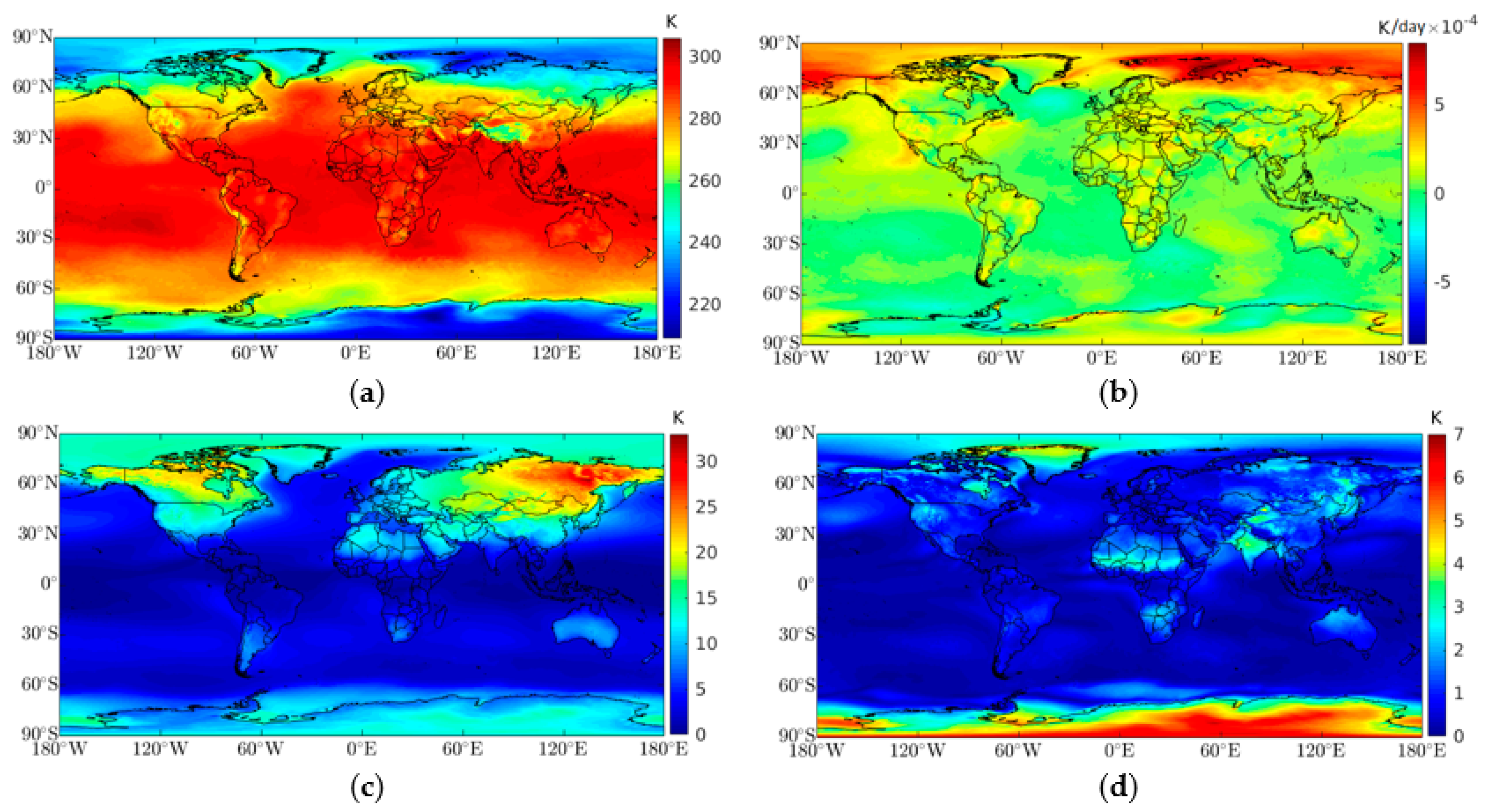
In this section, we present and discuss the mean global distribution of the and coefficient values, and each amplitude considered in the temperature and pressure models. The horizontal variation of the amplitude was analyzed at the ERA5 resolution (in comparison to the resolution used by the other models), and the introduction of a trend instead of the global mean was quantified. Figure 1 shows the global distribution of the mean coefficients of surface air temperature. The coefficient exhibited a minimum at the poles and a maximum near the equator, which also decreased with increasing altitude, e.g., such as in the Himalayas, Andes, or the Rocky Mountains (Figure 1a). This parameter approximately corresponded to the normal temperature profile, but it cannot be directly used as an indicator of the mean temperature. Globally, mean temperature trends were higher over continental areas than in sea areas, except for northern Russia (from Barents Sea to Chukchi Sea). Nevertheless, high-temperature trends were also observed over oceanic regions, such as the Pacific Ocean in the south of California and the Atlantic Ocean near the northeastern United States (Figure 1b).
Figure 1f shows the impact of introducing a linear trend in the temperature model as an alternative of just using the mean temperature. There was a difference of around 20% at the Equator and Colombia coast, 5% to 10% at the Pacific Ocean (between 10°S and 30°N), the Indian Ocean close to Madagascar, near the African Sahel, and at higher latitudes (northern Russia). Globally, there was a mean value close to 1%.
Regarding the seasonal components, Figure 1c shows that the annual amplitude increased with latitude and was larger for terrestrial areas, with the maximum amplitudes in Siberia, Mongolia, northeast of China, Alaska, and north of Canada. Figure 1d shows that the amplitude of the semi-annual component was larger over terrestrial areas, reaching maximum amplitudes over the Antarctic, but it was also significant for Greenland, the African Sahel, and India (due to the monsoons). The quarterly mean amplitude had a maximum value of 2 K over Siberia, and between 1 to 1.5 K in the east of Africa, specifically Ethiopia and Somalia, in the north of Canada, Himalayas, and some parts over Antarctic (Figure 1e). This periodicity was related to the major mode of tropical atmospheric variability on intraseasonal time scales, namely the Madden–Julian oscillation (MJO) system [30]. There was a large-scale link between the atmospheric circulation and tropical deep atmospheric convection, specifically in the northern temperate and polar zones, due to variations in the (1) Arctic oscillations, (2) rainfall in East Asia, (3) North American monsoon system, (4) Indian monsoon, and (5) surface air temperature at high latitudes in the Northern Hemisphere during winter [31,32]. Southern polar zone variations in the Antarctic oscillations are also related to the MJO [33]. Including this periodicity in the model led to an RMSE improvement of between 2.5% to 5% over the mentioned areas. Globally, the mean improvement due to the quarterly signal was 0.2%.
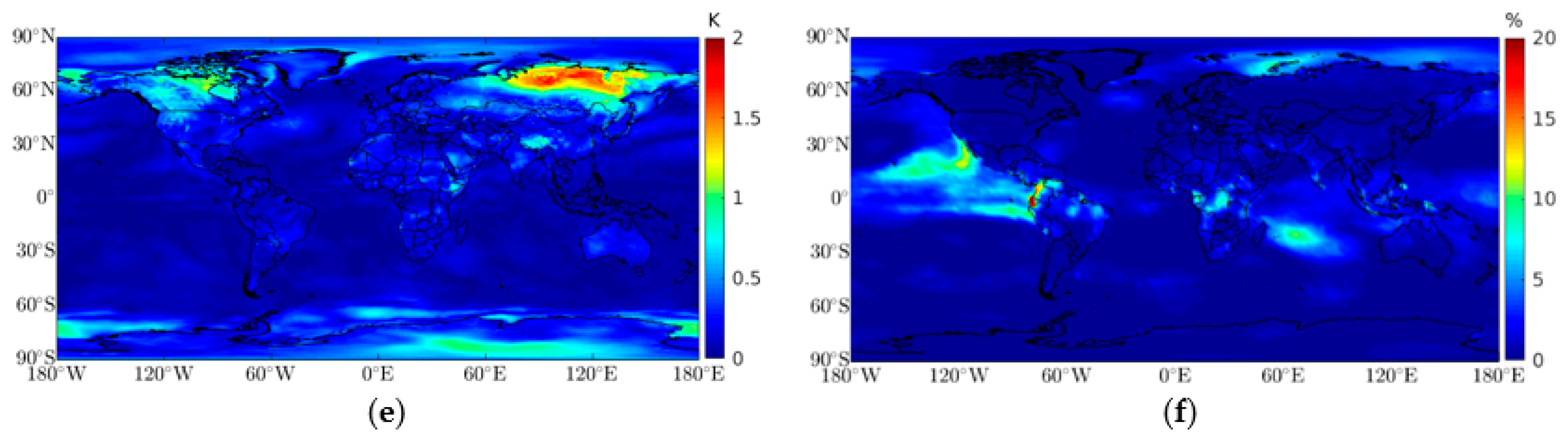
To further justify the high spatial resolution, the hourly mean maximum variability and standard deviation for each periodicity was calculated by using a window of 4 × 4 grid points, which was approximately the 1° × 1° horizontal grid that is normally adopted by other models. Figure 2 shows the maximum variability found for each amplitude. For the annual amplitude, differences up to 10 K in windows with a standard deviation of 4 K (not shown) were observed (Figure 2a). These variations were found along seacoasts, inland coasts, and around elevated areas, e.g., the Himalayas. These variations were expected in those areas due to complex weather dynamics between the ocean and land, or due to abrupt orographic changes, leading to larger temperature gradients in those areas. The semi-annual amplitude showed differences up to 3 K with a standard deviation of 1.5 K (Figure 2b). Larger values were found not only for the same places as in the annual amplitude differences, but also in elevated areas, e.g., Rocky Mountains, and near the equator, e.g., the African Sahel and northern South America. The quarterly amplitude showed differences up to 1 K with a standard deviation of 0.4 K for the same places (Figure 2c).
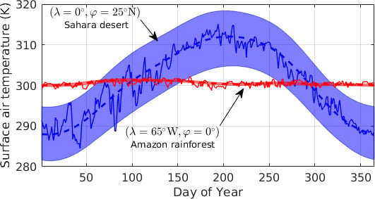
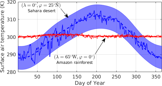
By combining the three seasonal components’ maximum values, we obtained a spatial temperature variation of 14 K inside a window of 1°. This variation could lead to a ZWD variation of up to 2.5 mm. A similar analysis was performed for the temporal resolution (not shown). We found 1-h variations up to 4 K for the annual amplitude in the west part of the United States and Canada, between 14:00 and 15:00 UTC. For the semi-annual amplitude, we found 1-h variations of up to 1.7 K over India, north of China, Mongolia, and Siberia, between 01:00 and 02:00 UTC. For the quarterly amplitude, 1-h variations reached 0.6 K over Siberia, between 21:00 and 22:00 UTC. The spatial and temporal variations found for the annual and semi-annual periodicities justified the use of the ERA5 full resolution model. It was obvious that the HGPT model not only improved the surface air temperature at seacoasts, where a considerable number of GNSS stations were available, but also the hydrological modeling at inland coasts. Considering the temperature of two locations with distinct climatological and topographical characteristics, for example, the Sahara desert (λ = 0°, φ = 25°N) and the Amazon Rainforest (λ = 65°W, φ = 0°) for a one-year time-span (2018), one can observe from Figure 3 that the time-segmentation model reproduced the diurnal cycle for both locations quite well.
The estimated coefficients for the surface pressure are shown in Figure 4. The coefficient values were lower inland and decreased considerably as the altitude increased, reaching a minimum in the Himalayas, followed by the Andes, the Antarctic, and Greenland. The mean trend for surface pressure was negative at the polar regions and positive in temperate zones. Introducing a linear trend in the pressure model as an alternative of just using the mean pressure led to an improvement of up to 5% in the Andes region, and about 2% in the Pacific and Atlantic Oceans, as well as some regions of Africa (Figure 4e). The mean annual amplitude was larger than 15 hPa in Greenland and parts of Asia, Australia, and some parts of the Antarctic (varies between 5 and 10 hPa), reaching a minimum near the equator. The mean semi-annual amplitude reached up to 4 hPa in the Antarctic and the southern and northern Pacific Ocean. To justify the high spatial and temporal resolutions, we performed the same analysis as described previously.
Figure 5 shows the maximum variability found for each amplitude. For the annual amplitude, we found differences of up to 12 hPa in windows with a standard deviation of 4.5 hPa (not shown). Most of these variations can be seen in Asia in the boundaries between plain and elevated areas. The semi-annual amplitude variations reached up to 2 hPa with a standard deviation of 0.5 hPa, which were located at seacoasts, mainly in the Antarctic and Greenland. Combining these differences could lead to variations of up to 32 mm in the ZHD using the Saastamoinen formula. Regarding the temporal resolution, we found 1-h variations for the annual amplitude of up to 1 hPa in some parts of Asia, the African Sahel, and in the Pacific Ocean between 09:00 and 10:00 UTC. The 1-h variations for the semi-annual amplitude reached 0.5 hPa in several locations, such as south of Africa, west of the United States, and in the southern Atlantic Ocean, for the same period.
The estimated regression coefficients, and , that were used in the estimation of the weighted mean temperature () from the surface air temperature () data are shown in Figure 6. The coefficient had a mean global value of 66.6 ± 17.5 K, a mean value of 97.6 ± 20.4 K over land, and a mean value of 45.9 ± 21.6 K over the ocean (Figure 6a). The coefficient also displayed an insignificant spatial variability for latitudes higher than 30°N and lower than 30°S; the largest variability in those regions was verified to be over the ocean. The coefficient showed a similar behavior, with a mean global value of 0.73 ± 0.06, a mean value of 0.61 ± 0.07 over land, and a mean value of 0.81 ± 0.07 over the ocean. Over land, and excluding the tropical zone, this coefficient displayed a slight variability, with a mean value of 0.63 ± 0.05 (Figure 6b). Around the equator (from 30°S to 30°N, i.e., the tropical zone), both coefficients showed a significant variability over both land and sea. This behavior can be explained in terms of the tropical atmospheric circulation (Hadley cells) and the ocean currents formed in this region, but more specifically by the Intertropical Convergence Zone (ITCZ) system. In tropical regions, the ITCZ transfers ocean heat and moisture from the lower levels of the atmosphere to the upper levels of the troposphere and to medium and high latitudes. These phenomena create rapid fluctuations in the air temperature and moisture with a slow impact on the surface air temperature. The ITCZ shifts during the year and tends to be located where the sun’s rays strike the ground more directly, i.e., during each hemisphere’s respective summers [34,35,36]. This phenomenon is easily identified in Figure 6c, where the distinct belts in both hemispheres stand out. Figure 6c shows the Pearson correlation coefficient between the , obtained using numerical integration, and the . It shows a mean global value of 0.82 ± 0.06, a mean value of 0.91 ± 0.10 over land, and a mean value of 0.79 ± 0.09 over the ocean. By removing the influence of the tropical zone, a stronger linear correlation (higher than 0.9) was obtained. Figure 6d shows the root mean square error (RMSE) between the obtained using a numerical integration and the calculated using the and coefficients, and the . We obtained a global error of 1.09 ± 0.08 K, an error of 1.28 ± 0.09 K over land, and an error of 0.99 ± 0.11 over the ocean. Areas with the highest RMSE values were Hudson Bay, connected to the Atlantic Ocean, showing lower salinity levels and covered by ice year-round, and therefore low evaporation rates, and the Okhotsk Sea, in the Pacific Ocean, also with low evaporation rates due to lower salinity levels and ice cover [37]. This can be an indicator of a deficient thermodynamic sea ice model simulation for large bays in the ERA5. However, this indicator needs further study to evaluate its feasibility, which is beyond the scope of this work.
Several studies have been carried out, using different techniques, to obtain , and several global and local models have been proposed. Bevis et al. [10] used 8718 radiosonde profiles at 13 U.S. sites over 2 years and proposed the following equation , which has been extensively used in GNSS meteorology, mainly in the Northern Hemisphere. Bevis [9] compared 502 radiosonde profiles with 12-h forecasts from the National Meteorological Center’s nested grid model to find an RMSE of 2.4 K and concluded that further improvements are possible with models at the highest resolutions. Mendes [3] proposed a linear model based on 32,500 radiosonde profiles over one year at 50 sites between 62°S and 83°N. Wang et al. [38] used the ERA40 reanalysis with a 1.125° × 1.125° grid, 60 hybrid vertical levels, and a 6-h temporal resolution to provide a global model. Yao et al. [39] combined radiosonde profiles with the GPT model to create virtual stations over sea, compensating for the lack of data in ocean areas. shows a substantial seasonal and geographic variability. The and values are more correlated in temperate zones and frigid zones, and less correlated in the tropic zone. Furthermore, the correlation tends to decrease in summer and increase in winter [40]. The same authors include the seasonal and geographic dependence in the regression coefficients, as well as regional models [41,42,43,44,45,46,47,48]. An assessment of global and regional models can be seen in References [40,49]. The PWV accuracy is proportional to the accuracy [9]. Improving the PWV accuracy is fundamental for severe weather monitoring and climate study, as the modeling still leaves considerable room for improvements when using high-resolution NWM data.
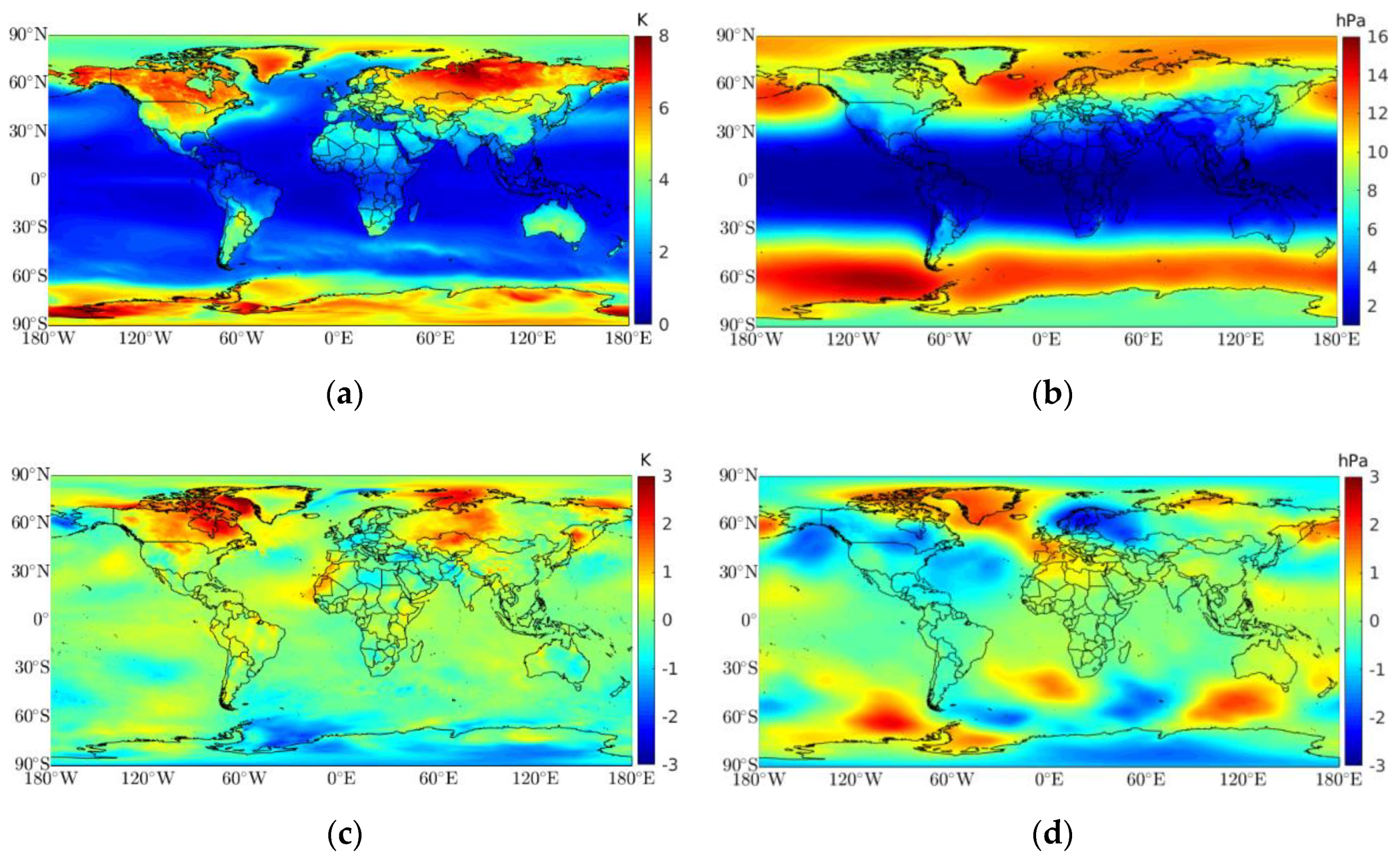
We validated the model by comparing the estimated model with the ERA5 surface air temperature and pressure. Figure 7 shows the mean global RMSE and the bias for both parameters. The temperature RMSE values increased as latitude increased, mostly over land, achieving a maximum value of 8 K (close to the Yenisei Gulf, Russia), and a maximum of 6 K over the ocean (in the Antarctic Ocean). It gave mean RMSEs of 4.8 ± 0.4 K, 1.9 ± 0.1 K, and 2.7 ± 0.2 K over land, over the ocean, and globally, respectively. The minimum RMSE values were observed in the tropical zone (as expected, due to the lower temperature variations). Canada, Alaska, Greenland, and Russia showed the worst RMSE, possibly due to the high surface air temperature variability at several temporal scales; furthermore, the air temperature has significantly increased in those regions in the last few decades in comparison to other regions [50,51,52]. Figure 7c shows the temperature bias spatial distribution, with a mean global value of 0.0 ± 0.6 K and a maximum absolute value of 2.8 K. Positive values indicate an HGPT model overestimation (e.g., northern of Canada and western Russia) and negative values indicate an underestimation (e.g., Antarctic regions). The pressure RMSE values also increased as latitude increased, but mostly over the ocean, achieving a maximum RMSE value of 16 hPa in the Antarctic Ocean, and a maximum of 13.4 hPa over land, in northern Russia. It gave mean RMSEs of 7.1 ± 1.0 hPa, 7.6 ± 0.8 hPa, and 7.1 ± 0.3 hPa over land, over the ocean, and globally, respectively. The worst RMSE values were found over the Antarctic Ocean, probably due to the complex atmospheric turbulence caused by the Antarctic circumpolar current (ACC) system [53], but also in the north of the Pacific and the Atlantic Oceans. Like temperature, the minimum RMSE values were found in the tropical zone. Figure 7d shows the pressure bias spatial distribution, with a mean global value of −0.1 ± 0.7 hPa and a maximum absolute value of 2.4 hPa. As stated previously, positive values indicate an HGPT model overestimation (e.g., Greenland) and negative values indicate an underestimation (e.g., western Russia and Scandinavia).
5. Accuracy Assessment
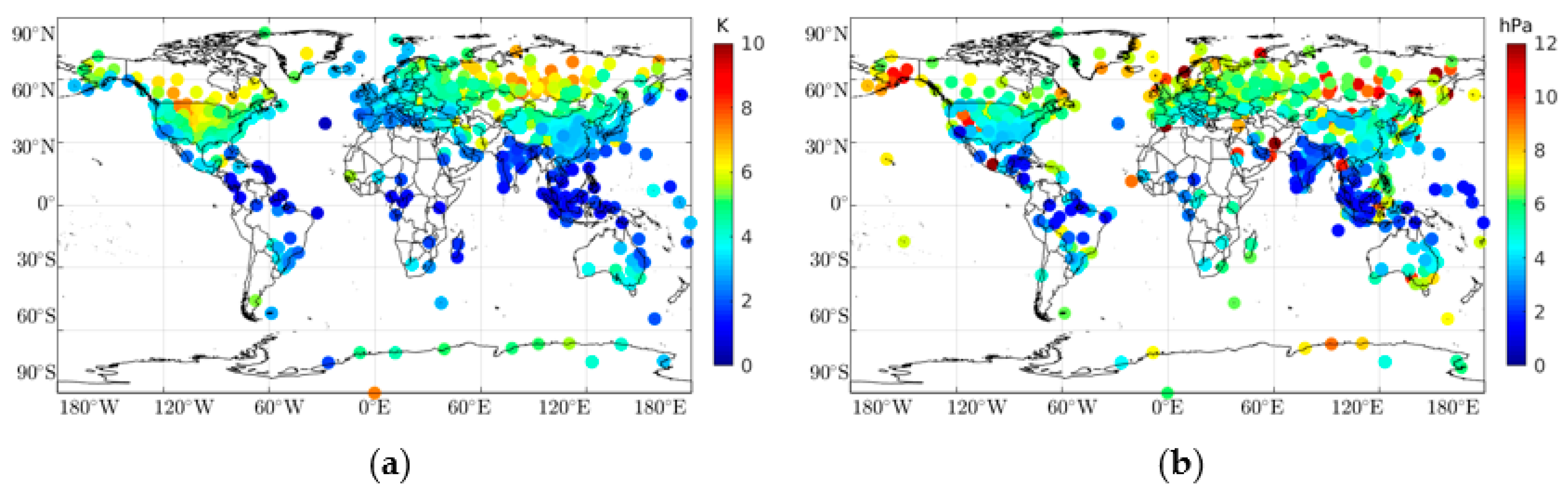
The accuracy assessment was performed using 510 radiosonde observations of surface air temperature and pressure available from the NOAA Integrated Global Radiosonde Archive (IGRA) version 2 [54]. We compared the first air temperature and pressure observations from each radiosonde data, classified as surface observations, for one year (2018), at 00:00 and 12:00 UTC, with the modeled air temperature and pressure values (bilinearly interpolated to the radiosonde sites). Figure 8 shows the RMSE distributions for temperature and pressure at 00:00 UTC. A mean RMSE value of 2.9 ± 1.6 K was obtained for the temperature, with a mean bias value of 0.5 ± 2.1 K. The highest RMSE values were found in the Northern Hemisphere, e.g., northern Russia and the Rocky Mountains. These locations displayed the largest annual amplitude variability compared with other locations (see Figure 1c). The lowest RMSE values were observed in the tropic zone. For the surface pressure, a mean RMSE value of 6.5 ± 2.5 hPa was obtained, with a mean bias value of −1.1 ± 3.8 hPa. The lowest RMSE values were found in the tropic zone. However, we obtained a more random pattern, probably linked to some pressure values, which was observed at different levels, and incorrectly registered as surface observations. A mean RMSE of 2.8 ± 1.5 K and a bias of 0.7 ± 2.0 K were obtained for the air temperature at 12:00 UTC, and a mean RMSE of 6.4 ± 3.1 hPa and a mean bias of −1.1 ± 4.1 K were obtained for the pressure at the same hour. We omitted the figure for this hour since the results were practically identical to those obtained at 00:00 UTC. To understand the magnitude of these values, we performed the same statistical analysis using the original signal from the ERA5 simulations. Table 1 shows the statistical summary obtained from the comparison between the radiosondes values and the HGPT and ERA5 models. On average, the ERA5 RMSE and bias values were about 40% lower when compared to the values obtained for the HGPT model.
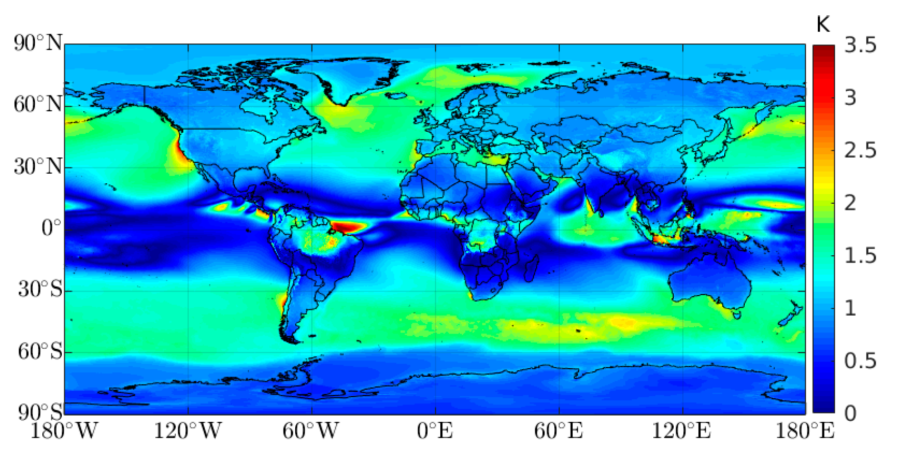
Yang et al. [23] compared five different models with distinct global temperature and pressure factors. The best global performance was achieved by a similar time-segmented model, fixing a 2-h temporal resolution and a 2.5° × 2° horizontal grid, obtaining a global RMSE of 2.95 ± 2.79 K and 7.87 ± 7.17 hPa for temperature and pressure, respectively. Comparing these results with the results of our study, we obtained an improvement of about 4% in the temperature estimation (from 2.95 ± 2.79 K to 2.85 ± 1.55 K) and about 18% in the pressure estimation (from 7.87 ± 7.17 hPa to 6.45±2.8 hPa). The ZHD can be predicted with a significant accuracy using the Saastamoinen model if accurate surface pressure measurements are available. A global standard deviation of 4.7 hPa was obtained from the difference between the HGPT model and the radiosonde observations. Appling the error propagation law to Equation (3), ignoring any possible errors in the latitude and height of each radiosonde station (Figure 8b), and adopting = 4.7 hPa, we obtained a ZHD global uncertainty of about 10 mm. Around 15% of the stations showed a standard deviation equal or lower than 0.5 hPa, leading to a ZHD uncertainty of about 1 mm. In a similar analysis for temperature, we found a global standard deviation of 1.5 K, and assuming there was no error in and (see Equation (6)), we obtained a global uncertainty of 1.1 K with a maximum value of 3.5 K over the Atlantic Ocean, close to the Amazon Rainforest (Figure 9).
Lan et al. [55] calculated linear regression coefficients between and at every 2° × 2.5° grid point using data from the ERA-Interim model and data from Global Geodetic Observing System (GGOS), and compared the results with the Constellation Observing System for Meteorology, Ionosphere, and Climate (COSMIC) and radiosonde data to obtain accuracies of 3.1 and 3.8 K, respectively. When compared with our results, we obtained a global accuracy improvement of about 33%.
6. Conclusions
In this work, we presented an ERA5-based hourly global pressure and temperature (HGPT) model. The HGPT model follows the time-segmentation concept and was based on 20 years of 0.25° × 0.25° spatial resolution and 1-h temporal resolution data from the ECMWF ERA5 reanalysis model. Its mathematical formulation includes a quarterly periodicity for temperature and a linear trend to account for a global climate change scenario. The model provides not only surface air temperature and pressure, but also a weighted mean temperature, as well as a zenith hydrostatic delay for any specific geographic location and time. The function coefficients are bilinearly interpolated in space using an efficient subroutine developed in Fortran, Matlab, and Python, which is available at https://github.com/pjmateus/hgpt_model, along with the coefficient files in binary format. The inclusion of a quarterly periodicity in modeling the surface air temperature improved the performance of the model by up to 5% at the highest latitudes. The use of a linear trend instead of a mean trend adopted by other models improved the performance of both temperature and pressure modeling by up to 20% and 5%, respectively. The spatial resolution that ERA5 offers will greatly improve the ZHD, mainly at seacoasts, where many GNSS stations are located, and in inland areas, enhancing hydrological modeling. The comparison of the HGPT and ERA5 models with observations of surface air temperature and pressure from 510 globally distributed radiosondes provided by IGRA showed a better performance of the ERA5 model. However, the differences between the two models in terms of RMSE and bias values were minimal. For the estimation of temperature, the RMSE value between the two models differed by 1.2 K, while their bias differed by 0.45 K. Likewise, for the pressure, we found differences of 2.7 hPa and 0.3 hPa. Globally, the ERA-based HGPT model increased the precision of the computation of the hydrostatic component by about 18%, equivalent to an increase in the precision of pressure when compared to other studies, which provided a corresponding increase of the precision in the estimate of the ZWD. Furthermore, an increase in the weighted mean temperature of about 33% compared to recent global models was obtained. As a consequence of the higher precision of the ZWD and , the precision of the estimated PWV increased.
Author Contributions
Conceptualization, software, investigation, resources, data curation, writing—original draft preparation, project administration, and funding acquisition: P.M.; Methodology and writing—review and editing: P.M., J.C., V.B.M., and G.N.; Validation: J.C., V.B.M., and G.N.; Formal analysis and supervision: J.C. All authors have read and agreed to the published version of the manuscript.
Funding
This research was funded by the OT4CLIMA Project, which was funded by the Italian Ministry of Education, University and Research (D.D. 2261 del 6.9.2018, PON R&I 2014–2020), and by FCT-Instituto Dom Luiz under Project UIDB/50019/2020 - IDL.
Acknowledgments
We are very grateful to Ricardo Tomé for his technical support and Ana Navarro for revising the text. We are grateful to the European Centre for Medium-Range Weather Forecasts (ECMWF) who have made the hourly climate simulations free and available, and to the Integrated Global Radiosonde Archive (IGRA), who also made the radiosonde observations and software free and available.
Conflicts of Interest
The authors declare no conflict of interest.
References
- Hofmann-Wellenhof, B.; Lichtenegger, H.; Wasle, E. GNSS—Global Navigation Satellite Systems. GNSS—Global Navigation Satellite Systems; Springer: Wien, Austria, 2008; p. 516. [Google Scholar]
- Xu, G. GPS: Theory, Algorithms and Applications; Springer: Berlin/Heidelberg, Germany, 2007; ISBN 9783540727149. [Google Scholar]
- Mendes, V.B. Modeling the Neutral-Atmospheric Propagation Delay in Radiometric Space Techniques; University of New Brunswick: Fredericton, NB, Canada, 1999; p. 353. [Google Scholar]
- Landskron, D.; Böhm, J. VMF3/GPT3: Refined discrete and empirical troposphere mapping functions. J. Geod. 2018, 92, 349–360. [Google Scholar] [CrossRef] [PubMed]
- Saastamoinen, J. Contributions to the theory of atmospheric refraction. J. Geod. 1972, 105, 279–298. [Google Scholar] [CrossRef]
- Hopfield, H.S. Two-quartic tropospheric refractivity profile for correcting satellite data. J. Geophys. Res. Space Phys. 1969, 74, 4487–4499. [Google Scholar] [CrossRef]
- Mateus, P.; Catalao, J.; Nico, G. Sentinel-1 Interferometric SAR Mapping of Precipitable Water Vapor Over a Country-Spanning Area. IEEE Trans. Geosci. Remote. Sens. 2017, 55, 2993–2999. [Google Scholar] [CrossRef]
- Mendes, V.; Langley, R.B. Tropospheric Zenith Delay Prediction Accuracy for High-Precision GPS Positioning and Navigation. Navig. 1999, 46, 25–34. [Google Scholar] [CrossRef]
- Bevis, M. GPS meteorology: Mapping zenith wet delays onto precipitable water. J. Appl. Meteorol. 1994, 33, 379–386. [Google Scholar] [CrossRef]
- Bevis, M.; Businger, S.; Herring, T.; Rocken, C.; Anthes, R.A.; Ware, R.H. GPS meteorology: Remote sensing of atmospheric water vapor using the global positioning system. J. Geophys. Res. Space Phys. 1992, 97, 15787. [Google Scholar] [CrossRef]
- Collins, J.P. Assessment and Development of a Tropospheric Delay Model for Aircraft Users of the Global Positioning System; University of New Brunswick: Fredericton, NB, Canada, 1999; p. 174. [Google Scholar]
- Leandro, R.F.; Langley, R.B.; Santos, M.C. UNB3m_pack: A neutral atmosphere delay package for radiometric space techniques. GPS Solut. 2007, 12, 65–70. [Google Scholar] [CrossRef]
- Boehm, J.; Heinkelmann, R.; Schuh, H.; Böhm, J. Short Note: A global model of pressure and temperature for geodetic applications. J. Geod. 2007, 81, 679–683. [Google Scholar] [CrossRef]
- Lagler, K.; Schindelegger, M.; Böhm, J.; Krasna, H.; Nilsson, T. GPT2: Empirical slant delay model for radio space geodetic techniques. Geophys. Res. Lett. 2013, 40, 1069–1073. [Google Scholar] [CrossRef] [Green Version]
- Böhm, J.; Moeller, G.; Schindelegger, M.; Pain, G.; Weber, R. Development of an improved empirical model for slant delays in the troposphere (GPT2w). GPS Solut. 2014, 19, 433–441. [Google Scholar] [CrossRef] [Green Version]
- Schüler, T. The TropGrid2 standard tropospheric correction model. GPS Solut. 2013, 18, 123–131. [Google Scholar] [CrossRef]
- Martellucci, A.; Cerdeira, A.R.P. Review of tropospheric, ionospheric and multipath data and models for global navigation satellite systems. In Proceedings of the European Conference on Antennas and Propagation, EuCAP 2009, Proceedings; EurAAP, Berlin, Germany, 23–27 March 2009; pp. 3697–3702. [Google Scholar]
- Yao, Y.; Xu, C.; Shi, J.; Cao, N.; Zhang, B.; Yang, J. ITG: A New Global GNSS Tropospheric Correction Model. Sci. Rep. 2015, 5, 10273. [Google Scholar] [CrossRef] [PubMed] [Green Version]
- Stull, R.B. An Introduction to Boundary Layer Meteorology; Springer: Amsterdam, The Netherlands, 1988. [Google Scholar]
- Saastamoinen, J.; Henriksen, S.W.; Mancini, A.; Chovitz, B.H. Atmospheric Correction for the Troposphere and Stratosphere in Radio Ranging Satellites. Sea Ice 2013, 15, 247–251. [Google Scholar]
- Davis, J.L.; Herring, T.; Shapiro, I.I.; Rogers, A.E.E.; Elgered, G. Geodesy by radio interferometry: Effects of atmospheric modeling errors on estimates of baseline length. Radio Sci. 1985, 20, 1593–1607. [Google Scholar] [CrossRef]
- Tuka, A.; El-Mowafy, A. Performance evaluation of different troposphere delay models and mapping functions. Measurement 2013, 46, 928–937. [Google Scholar] [CrossRef] [Green Version]
- Yang, F.; Meng, X.; Guo, J.; Shi, J.; An, X.; He, Q.; Zhou, L. The Influence of Different Modelling Factors on Global Temperature and Pressure Models and Their Performance in Different Zenith Hydrostatic Delay (ZHD) Models. Remote. Sens. 2019, 12, 35. [Google Scholar] [CrossRef] [Green Version]
- Rüeger, J.M.; Jean Rüeger, A.M. Refractive Index Formulae for Radio Waves. In Proceedings of the FIG XXII International Congress, Washington, DC, USA, 19–26 April 2002; pp. 19–26. [Google Scholar]
- Copernicus Climate Change Service (C3S). ERA5: Fifth generation of ECMWF atmospheric reanalyses of the global climate. Available online: https://cds.climate.copernicus.eu/cdsapp#!/home (accessed on 29 January 2020).
- Hoffman, L.; Günther, G.; Li, D.; Stein, O.; Wu, X.; Griessbach, S.; Heng, Y.; Konopka, P.; Müller, R.; Vogel, B.; et al. From ERA-Interim to ERA5: The considerable impact of ECMWF’s next-generation reanalysis on Lagrangian transport simulations. Atmospheric Chem. Phys. Discuss. 2019, 19, 3097–3124. [Google Scholar] [CrossRef] [Green Version]
- Hersbach, H.; Bell, B.; Berrisford, P.; Horányi, A.; Sabater, J.M.; Nicolas, J.; Radu, R.; Schepers, D.; Simmons, A.; Soci, C.; et al. Global Reanalysis: Goodbye ERA-Interim, Hello ERA5. ECMWF Newsl. 2019. Available online: https://www.ecmwf.int/en/newsletter/159/meteorology/global-reanalysis-goodbye-era-interim-hello-era5 (accessed on 28 January 2020).
- European Centre for Medium-Range Weather Forecasts (ECMWF). Part IV: Physical Processes. IFS Doc. CY41R2 2016, 213. Available online: https://www.ecmwf.int/sites/default/files/elibrary/2016/17117-part-iv-physical-processes.pdf (accessed on 25 January 2020).
- Lemoine, F.G.; Smith, D.E.; Kunz, L.; Smith, R.; Pavlis, E.C.; Pavlis, N.K.; Klosko, S.M.; Chinn, D.S.; Torrence, M.H.; Williamson, R.G.; et al. The Development of the NASA GSFC and NIMA Joint Geopotential Model. Int. Assoc. Geod. Symp. 1997, 117, 461–469. [Google Scholar]
- Zhang, C. Madden-Julian Oscillation. Rev. Geophys. 2005, 43, 1–36. [Google Scholar] [CrossRef] [Green Version]
- Zhou, Y.; Thompson, K.R.; Lu, Y. Mapping the Relationship between Northern Hemisphere Winter Surface Air Temperature and the Madden–Julian Oscillation. Mon. Weather. Rev. 2011, 139, 2439–2454. [Google Scholar] [CrossRef]
- Zhou, Y.; Lu, Y.; Yang, B.; Jiang, J.; Huang, A.; Zhao, Y.; La, M.; Yang, Q. On the relationship between the Madden-Julian Oscillation and 2 m air temperature over central Asia in boreal winter. J. Geophys. Res. Atmos. 2016, 121, 13–250. [Google Scholar] [CrossRef] [Green Version]
- Flatau, M.; Kim, Y.-J. Interaction between the MJO and Polar Circulations. J. Clim. 2013, 26, 3562–3574. [Google Scholar] [CrossRef]
- Hess, P.G.; Dbattisti, D.S.; Rasch, P.J. Maintenance of the Intertropical Convergence Zones and the Large-Scale Tropical Circulation on a Water-covered Earth. J. Atmospheric Sci. 1993, 50, 691–713. [Google Scholar] [CrossRef] [Green Version]
- Waliser, D.E.; Somerville, R.C.J. Preferred Latitudes of the Intertropical Convergence Zone. J. Atmospheric Sci. 1994, 51, 1619–1639. [Google Scholar] [CrossRef] [Green Version]
- Chao, W.C.; Chen, B. Single and double ITCZ in an aqua-planet model with constant sea surface temperature and solar angle. Clim. Dyn. 2004, 22, 447–459. [Google Scholar] [CrossRef]
- Al-Shammiri, M. Evaporation rate as a function of water salinity. Desalination 2002, 150, 189–203. [Google Scholar] [CrossRef]
- Wang, J.; Zhang, L.; Dai, A. Global estimates of water-vapor-weighted mean temperature of the atmosphere for GPS applications. J. Geophys. Res. Space Phys. 2005, 110, 1–17. [Google Scholar] [CrossRef] [Green Version]
- Yao, Y.; Zhu, S.; Yue, S. A globally applicable, season-specific model for estimating the weighted mean temperature of the atmosphere. J. Geod. 2012, 86, 1125–1135. [Google Scholar] [CrossRef]
- Ross, R.J.; Rosenfeld, S. Estimating mean weighted temperature of the atmosphere for Global Positioning System applications. J. Geophys. Res. Space Phys. 1997, 102, 21719–21730. [Google Scholar] [CrossRef] [Green Version]
- Emardson, T.R.; Derks, H.J.P. On the relation between the wet delay and the integrated precipitable water vapour in the European atmosphere. Meteorol. Appl. 2000, 7, 61–68. [Google Scholar] [CrossRef]
- Isioye, O.; Combrinck, L.; Botai, J. Modelling weighted mean temperature in the West African region: Implications for GNSS meteorology. Meteorol. Appl. 2016, 23, 614–632. [Google Scholar] [CrossRef]
- Mateus, P.; Nico, G.; Catalao, J. Maps of PWV Temporal Changes by SAR Interferometry: A Study on the Properties of Atmosphere’s Temperature Profiles. IEEE Geosci. Remote. Sens. Lett. 2014, 11, 2065–2069. [Google Scholar] [CrossRef]
- Singh, D.; Ghosh, J.; Kashyap, D. Weighted mean temperature model for extra tropical region of India. J. Atmos. Solar Terr. Phys. 2014, 107, 48–53. [Google Scholar] [CrossRef]
- Zhang, F.; Barriot, J.-P.; Xu, G.; Yeh, T.-K. Metrology Assessment of the Accuracy of Precipitable Water Vapor Estimates from GPS Data Acquisition in Tropical Areas: The Tahiti Case. Remote. Sens. 2018, 10, 758. [Google Scholar] [CrossRef] [Green Version]
- Liou, Y.-A.; Teng, Y.-T.; Van Hove, T.; Liljegren, J.C. Comparison of Precipitable Water Observations in the Near Tropics by GPS, Microwave Radiometer, and Radiosondes. J. Appl. Meteorol. 2001, 40, 5–15. [Google Scholar] [CrossRef]
- Raju, C.S.; Saha, K.; Thampi, B.V.; Parameswaran, K. Empirical model for mean temperature for Indian zone and estimation of precipitable water vapor from ground based GPS measurements. Ann. Geophys. 2007, 25, 1935–1948. [Google Scholar] [CrossRef] [Green Version]
- Yao, Y.; Zhang, B.; Yue, S.Q.; Xu, C.; Peng, W.F. Global empirical model for mapping zenith wet delays onto precipitable water. J. Geod. 2013, 87, 439–448. [Google Scholar] [CrossRef]
- Mendes, V.B.; Prates, G.; Santos, L.; Langley, R.B. An Evaluation of the Accuracy of Models for the Determination of the Weighted Mean Temperature of the Atmosphere. In Proceedings of the Institute of Navigation 2000 National Technical Meeting, Anaheim, CA, USA, 26–28 January 2000; pp. 3–8. [Google Scholar]
- Vincent, L.A.; Zhang, X.; Brown, R.D.; Feng, Y.; Mekis, E.; Milewska, E.J.; Wan, H.; Wang, X.L. Observed Trends in Canada’s Climate and Influence of Low-Frequency Variability Modes. J. Clim. 2015, 28, 4545–4560. [Google Scholar] [CrossRef]
- Babina, E.D.; Semenov, V.A. Intramonthly Variability of Daily Surface Air Temperature in Russia in 1970–2015. Russ. Meteorol. Hydrol. 2019, 44, 513–522. [Google Scholar] [CrossRef]
- Kobashi, T.; Goto-Azuma, K.; Box, J.; Gao, C.-C.; Nakaegawa, T. Causes of Greenland temperature variability over the past 4000 yr: Implications for northern hemispheric temperature changes. Clim. Past 2013, 9, 2299–2317. [Google Scholar] [CrossRef] [Green Version]
- Rintoul, S.R.; Hughes, C.W.; Olbers, D. Chapter 4.6 The antarctic circumpolar current system. Int. Geophys. 2001, 77, 271. [Google Scholar]
- Durre, I.; Yin, X. Enhanced Radiosonde Data For Studies of Vertical Structure. Bull. Am. Meteorol. Soc. 2008, 89, 1257–1262. [Google Scholar] [CrossRef]
- Lan, Z.; Zhang, B.; Geng, Y. Establishment and analysis of global gridded Tm− Ts relationship model. Geodesy Geodyn. 2016, 7, 101–107. [Google Scholar] [CrossRef] [Green Version]
Figure 1.
Global distribution of mean coefficients for surface air temperature. The globe was divided into a 0.25° × 0.25° grid. (a)
mean values (K), (b)
mean values (trend) (K/day), (c) mean annual amplitude contribution (K), (d) mean semi-annual contribution (K), (e) mean quarterly contribution (K); and (f) mean impact of introducing a linear trend versus using only the mean temperature, in percentage.


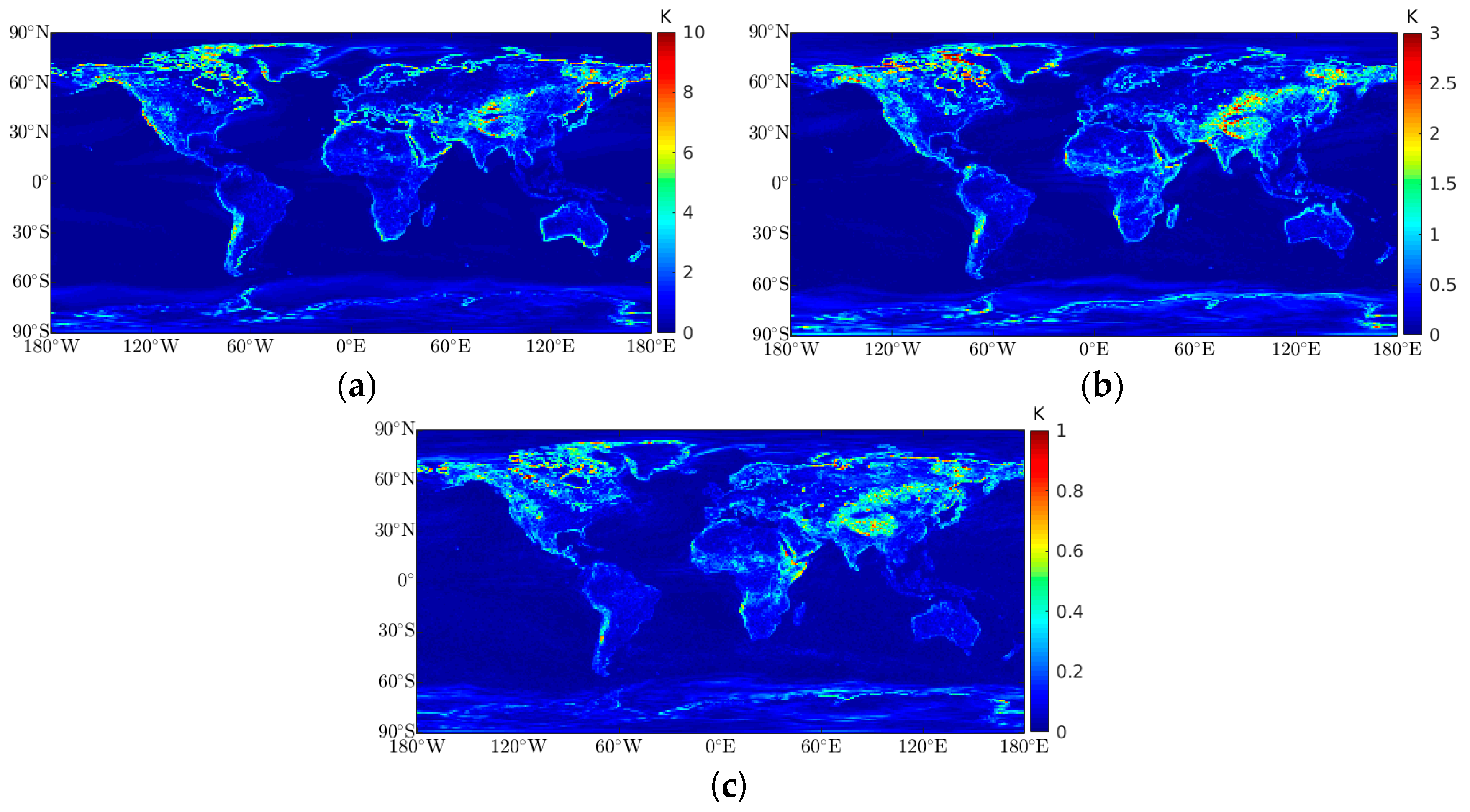
Figure 2.
Maximum spatial variability for each surface air temperature periodicity, which was calculated using a window of 4 × 4 grid points, approximately a 1° × 1° horizontal grid: (a) maximum spatial variability for the annual amplitude (K), (b) maximum spatial variability for the semi-annual amplitude (K), and (c) maximum spatial variability for the quarterly amplitude (K).

Figure 3.
Surface air temperature at two distinct locations (different climatological and topographical characteristics). In blue: over the Sahara Desert (λ = 0°, φ = 25°N), and in red: over the Amazon Rainforest (λ = 65°W, φ = 0°) for a one-year timespan (2018). The bluish shaded area represents the diurnal cycle. The dashed line represents the model daily mean and the continuous line represents the daily mean of all ERA5 simulations (24 time series, each one represents one hour).

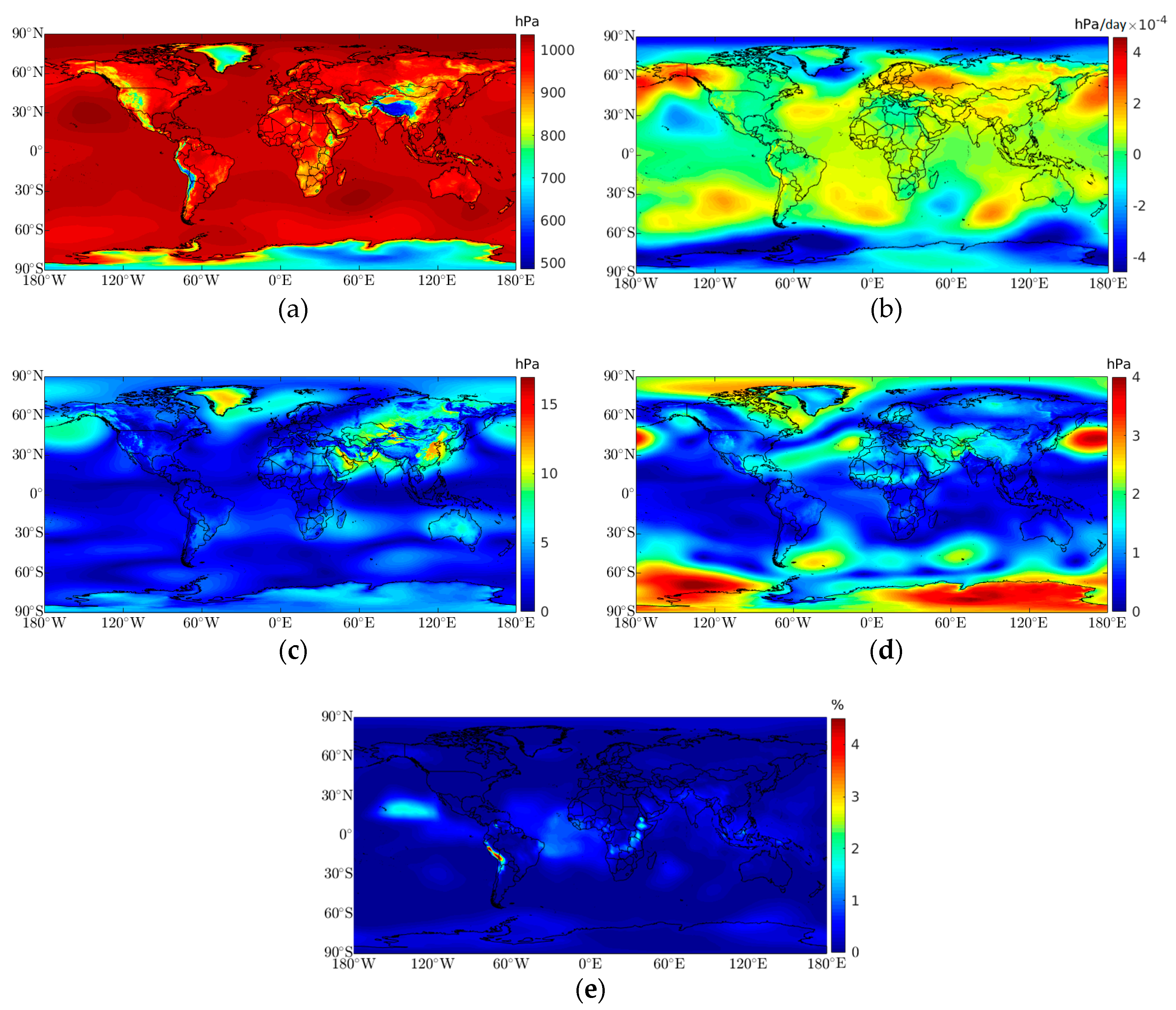
Figure 4.
Global distribution of mean coefficients for surface pressure. The globe was divided into a grid of 0.25° × 0.25°. (a)
mean values (hPa), (b) mean values (trend) (hPa/day), (c) contribution from the annual mean amplitude (hPa), (d) contribution from the semi-annual mean amplitude (hPa), and (e) mean impact of introducing a linear trend versus using only the mean pressure (%).

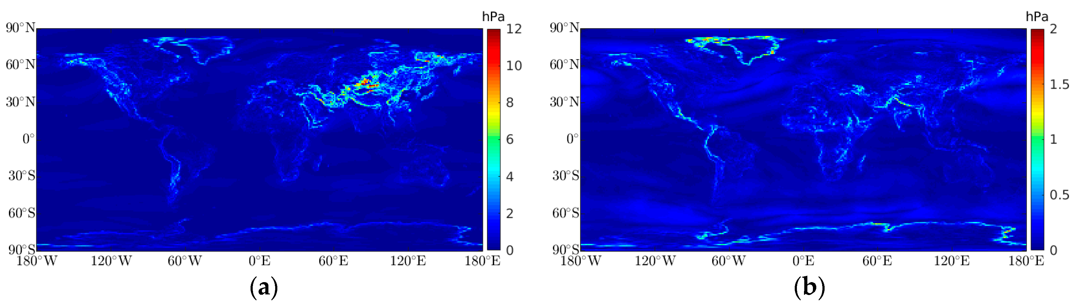
Figure 5.
Maximum spatial variability for each surface pressure periodicity, which were calculated using a window of 4 × 4 grid points, approximately a 1° × 1° horizontal grid: (a) maximum spatial variability for the annual amplitude (hPa) and (b) maximum spatial variability for semi-annual amplitude (hPa).

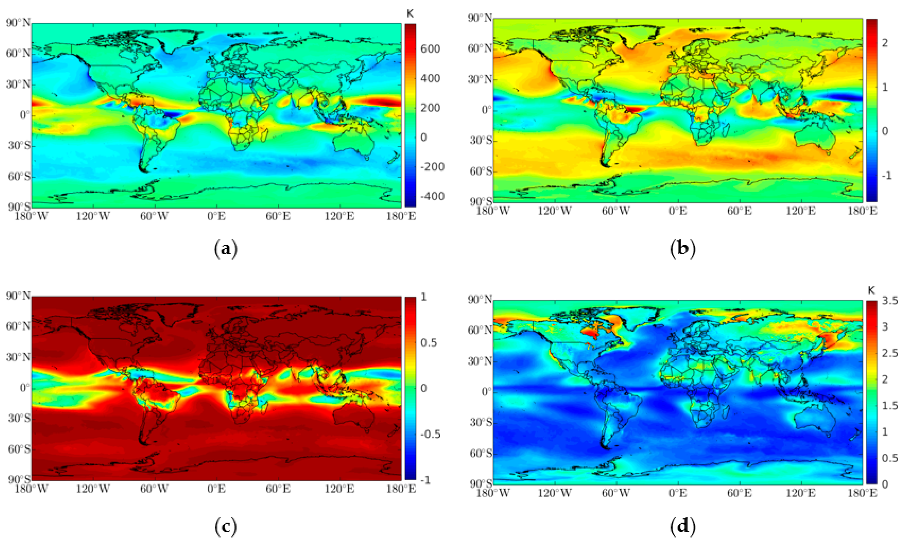
Figure 6.
(a,b)
and regression coefficients, obtained using 20 years of monthly ERA5 data, which were used to estimate the weighted mean temperature () from the surface air temperature (). (c) Pearson correlation coefficient between the obtained using ERA5 numerical integration at each grid point and . (d) RMSE between obtained using , , and , and the obtained using ERA5’s numerical integration (see Equation (5)). The estimation of the coefficients in the tropic regions could generate artefacts, especially over the sea, when did not vary over a range large enough to get a satisfactory estimation of the parameters.

Figure 7.
Comparison of 20 years of ERA5 surface air temperature and pressure with the modeled values using Equations (1) and (2): (a) mean RMSE for surface air temperature (K), (b) mean RMSE for surface pressure (hPa), (c) mean bias for surface air temperature (K), and (d) mean bias for surface pressure (hPa). Note that a positive bias value indicates an hourly global pressure and temperature (HGPT) model overestimation and a negative bias value indicates an underestimation.

Figure 8.
Global distribution of the mean RMSE values: (a) mean RMSEs for surface air temperature at 00:00 UTC (K) and (b) mean RMSEs for surface pressure at 00:00 UTC (hPa).
Figure 8.
Global distribution of the mean RMSE values: (a) mean RMSEs for surface air temperature at 00:00 UTC (K) and (b) mean RMSEs for surface pressure at 00:00 UTC (hPa).

Figure 9.
Accuracy spatial distribution for
considering a global standard deviation of 1.1 K for surface air temperature and ignoring possible errors in and .
Figure 9.
Accuracy spatial distribution for
considering a global standard deviation of 1.1 K for surface air temperature and ignoring possible errors in and .


Table 1.
Statistical analysis. RMSE and bias values (with standard deviation) between the HGPT model and radiosondes and the original signal (ERA5 simulations) and radiosondes, for 00:00 and 12:00 UTC. A negative bias indicates overestimation by the HGPT or ERA5 models and a negative bias indicates an underestimation.
| 00:00 UTC | 12:00 UTC | |||||||
|---|---|---|---|---|---|---|---|---|
| RMSE | Bias | RMSE | Bias | |||||
| HGPT | ERA5 | HGPT | ERA5 | HGPT | ERA5 | HGPT | ERA5 | |
| T (K) | 2.9 ± 1.6 | 1.7 ± 0.7 | 0.5 ± 2.1 | −0.1 ± 1.2 | 2.8 ± 1.5 | 1.6 ± 0.7 | 0.7 ± 2.0 | −0.2 ± 1.9 |
| P (hPa) | 6.5 ± 2.5 | 3.8 ± 3.2 | −1.1 ± 3.8 | −0.7 ± 4.7 | 6.4 ± 3.1 | 3.7 ± 3.4 | −1.1 ± 4.1 | −0.9 ± 4.7 |
© 2020 by the authors. Licensee MDPI, Basel, Switzerland. This article is an open access article distributed under the terms and conditions of the Creative Commons Attribution (CC BY) license (http://creativecommons.org/licenses/by/4.0/).
Share and Cite
MDPI and ACS Style
Mateus, P.; Catalão, J.; Mendes, V.B.; Nico, G. An ERA5-Based Hourly Global Pressure and Temperature (HGPT) Model. Remote Sens. 2020, 12, 1098. https://doi.org/10.3390/rs12071098
AMA Style
Mateus P, Catalão J, Mendes VB, Nico G. An ERA5-Based Hourly Global Pressure and Temperature (HGPT) Model. Remote Sensing. 2020; 12(7):1098. https://doi.org/10.3390/rs12071098
Chicago/Turabian StyleMateus, Pedro, João Catalão, Virgílio B. Mendes, and Giovanni Nico. 2020. "An ERA5-Based Hourly Global Pressure and Temperature (HGPT) Model" Remote Sensing 12, no. 7: 1098. https://doi.org/10.3390/rs12071098
Note that from the first issue of 2016, this journal uses article numbers instead of page numbers. See further details here.