
Abstract
Multidimensional numeric arrays are often serialized to binary formats for efficient storage and processing. These representations can be stored as binary objects in existing relational database management systems. To minimize data transfer overhead when arrays are large and only parts of arrays are accessed, it is favorable to split these arrays into separately stored chunks. We process queries expressed in an extended graph query language SPARQL, treating arrays as node values and having syntax for specifying array projection, element and range selection operations as part of a query. When a query selects parts of one or more arrays, only the relevant chunks of each array should be retrieved from the relational database. The retrieval is made by automatically generated SQL queries. We evaluate different strategies for partitioning the array content, and for generating the SQL queries that retrieve it on demand. For this purpose, we present a mini-benchmark, featuring a number of typical array access patterns. We draw some actionable conclusions from the performance numbers.
1 Introduction
Many scientific and engineering applications involve storage and processing of massive numeric data in the form of multidimensional arrays. These include satellite imagery, climate studies, geosciences, and generally any spatial and spatiotemporal simulations and instrumental measurements [1], computational fluid dynamics and finite element analysis. The need for efficient representation of numeric arrays has been driving the scientific users away from the existing DBMS solutions [2], towards more specialized file-based data representations. The need for integrated and extensible array storage and processing framework supporting queriable metadata are our main motivations for the development of Scientific SPARQL: an extension of W3C SPARQL language [3] with array functionality.
Within the Scientific SPARQL project [4–8], we define syntax and semantics for queries combining both RDF-structured metadata and multidimensional numeric arrays which are linked as values in the RDF graph. Different storage options are explored: our prior publications cover storing arrays in binary files [6], and a specialized array database [7]. In this work we focus on storing the arrays in a relational DBMS back-end. Scientific SPARQL Database Manager (SSDM) implements the query language, in-memory and external array storage, along with the extensibility interfaces. The software and documentation are available at the project homepage [9].
The contributions presented in this work are the following:
A framework for processing array data retrieval queries, which allows adaptive pattern discovery, pre-fetching of chunks from external storage;
A mini-benchmark featuring the typical and diverse array access patterns;
Evaluation of different array data retrieval strategies under different array data partitioning options and access patterns, and the conclusions drawn regarding the workload-aware partitioning options, suggestions for building array processing infrastructures, and estimates of certain trade-offs.
In this work we consider an SSDM configuration where array data is partitioned into BLOBs in a back-end relational database. An SSDM server provides scalable processing of SciSPARQL queries which can be expressed both in terms of metadata conditions (pattern matching, filters) and functions over the numeric data (filters, aggregation). SciSPARQL queries allow specifying array projection, element and range selection operations over the arrays, thus defining (typically, sparse) access patterns to the dense multidimensional arrays.
The techniques presented here are language-independent, and can be applied to the processing of any array query language which has these basic array operations. Typical queries which benefit from these optimizations are characterized by (1) accessing relatively small portions of the arrays, and (2) accessing array elements based on subscript expressions or condition over subscripts, rather than the element values.
The rest of this paper is structured as follows: Sect. 2 summarizes the related work, in Sect. 3 we begin with an example, and then give an overview of the array query processsing technique, namely, array proxy resolution. Section 4 lists different ways (strategies) to generate SQL queries that will be sent to the DBMS back-end to retrieve the chunks, and Sect. 5 describes our Sequence Pattern Detector algorithm (SPD) used in one of these strategies. Section 6 offers the evaluation of different array storage and array data retrieval strategies using a mini-benchmark, featuring a number of typical array access patterns expressed as parameterized SciSPARQL queries. Section 7 concludes the results and suggests the way they can be applied in array storage and query processing solutions.
2 Background and related work
There are several systems and models of integrating arrays into other database paradigms, in order ot allow array queries which utilize metadata context. There are two major approaches: first is normalizing the arrays in terms of the host data model, as represented by SciQL [10], along with its predecessor RAM [11], where array is an extension of the relation concept. Data Cube Vocabulary [12] suggests a way to represent multidimensional statistical data in terms of an RDF graph, which can be handled by any RDF store. The second approach is incorporation of arrays as value types—this includes PostgreSQL [13], recent development of ASQL [2] on top of Rasdaman [14], as well as extensions to MS SQL Server based on BLOBs and UDFs, e.g. [15].
We follow the second approach in the context of Semantic Web, offering separate sets of query language features for navigating graphs and arrays. Surprisingly, many scientific applications involving array computations and storage do not employ any DBMS infrastructures, and hence cannot formulate array queries. Specialized file formats (e.g. NetCDF [16]) or hierarchical databases (e.g. ROOT [17]) are still prevalent in many domains. Parallel processing frameworks are also being extended to optimize the handling array data in files—see e.g. SciHadoop [18]. Storing arrays in files has its own benefits, e.g. eliminating the need for data ingestion, as shown by comparison of SAGA to SciDB [19]. The SAGA system takes a step to bridge the gap between file-resident arrays and optimizable queries. SciSPARQL also incorporates the option of file-based array storage, as presented in the context of its tight integration into Matlab [6]. Still, in the present technological context we believe that utilizing a state-of-the-art relational DBMS to store massive array data promises better scalability, thanks to cluster and cloud deployment of these solutions, and mature partitioning and query parallelization techniques.
Regarding the storage approaches, in this work we explore two basic partitioning techniques—simple chunking of the linearized form of array (which, we believe, is a starting reference point for any ad-hoc solution), and more advanced multidimensional tiling used e.g. in Rasdaman [20, 21], ArrayStore [22], RIOT [23], and SciDB [19] which helps preserving access locality to some extent. We do not implement a language for user-defined tiling, as this concept has been already explored in Rasdaman [20]. While cleverly designed tiling increases the chances of an access pattern to become regular, it still has to be made manually and beforehand, with expected workload in mind. With the SPD algorithm we are able to discover such regularity during the query execution.
In this work we only study sparce array access to the dense stored arrays and we use a relational DBMS back-end to store the chunks, in contrast to stand-alone index data structures employed by ROOT [23] and ArrayStore [22]. Apart from utilizing DBMS for scalability, does not make much difference in finding the optimal way to access the array data. As the SAGA evaluation [24] has shown, even in the absence of SQL-based back-end integration, the sequential access to chunks provides a substantial performance boost over the random access.
3 The problem of retrieving array content
Scientific SPARQL, as many other array processing languages (Matlab, SciPy) and query languages [14, 19, 10, 2] do, allows the specification of subarrays by supplying subscripts or ranges independently for different array dimensions. We distinguish the projection operations that reduce the array dimensionality, like ?A[i], selecting an (n−1)-dimensional slice from an n-dimensional array bound to ?A (or a single element if ?A is 1-dimensional) and range selection operations like ?A[lo:stride:hi]. All array subscripts are 1-based, and hi subscript is included into the range. Any of lo, stride, or hi can be omitted, defaulting to index 1, stride of 1, and array size in that dimension respectively.
Let us consider the following SciSPARQL query Q1 selecting equally spaced elements from a single column of a matrix, which is found as a value of the :result property of the : Sim1 node.

We assume the dataset includes the following RDF with Arrays triple, containing a 10 × 10 array as its value, as in Fig. 1a, the subset retrieved by Q1 is shown hatched.

An RDF with Arrays dataset using a linear and b multidimensional partitioning
In our relational back-end this array is stored in 20 linear chunks, containing 5 elements each (chunk ids shown on the picture). Figure 1b shows a variant of the same dataset, where the array is stored in 25 2 × 2 non-overlapping square tiles. The example (a) is used through the rest of this section, and we compare the two storage approaches in Sect. 6.
In our setting the RDF metadata triples have considerably smaller volume than the ‘real’ array data, so they can be cached in main memory to speedup matching and joining the triple patterns. Our problem in focus is querying the big ArrayChunks(arrayid, chunkid, chunk) table in the relational back-end, in order to extract data from the array. In general, we would like to (1) minimize the number of SQL queries (round-trips) to ArrayChunks, and (2) minimize the amount of irrelevant data retrieved.
3.1 Array query processing overview
There are a number of steps to be performed before the back-end will be queried for the actual array content:
Identifying the set of array elements that are going to be accessed while processing an array query. Such sets of elements are described with bags of array proxy objects, which represent derived arrays or single elements, which are stored in an external system. We refer to the process of turning array proxies into in-memory arrays as Array Proxy Resolution (APR).
The array proxies accumulate array dereference and transposition operations. An enumerable set of array proxies can be generated using free index variables, as shown in by QT4 in the Table 2.
Identifying fragments of the derived array to be retrieved that are contiguous in the linearized representation of the original array in order to save on the number of data-transfer operations.
Identifying array chunks needed to be retrieved and formulating data transfer operations for each chunk. Buffering these chunk ids and data transfer operations.
Formulating SQL queries to the back-end RDBMS, as explained in the next section.
If the formulated SQL query is prediction-based (e.g. generated with SPD strategy, as described below), switching between the phases of (I) simulation, i.e. translating elements/fragments to chunk ids, and buffering, (II) performing the buffered operations, and (III) performing the further (unbuffered) operations, as long as the prediction-based query yields the relevant chunks. This includes taking care of false-positives and false-negatives.
As the input of this process is a stream of array proxies generated during SciSPARQL query execution, the output is the stream of corresponding in-memory arrays. Essential parts of this process are described in our previous works [4, 5].
4 Strategies for formulating SQL queries during APR
There are a number of possible strategies to translate sets of chunk ids in the buffer to SQL queries retrieving the relevant chunks. The basic one we are about to study are:
NAIVE: send a single SQL query for each chunk id. This proves to be unacceptably slow in realistic data volumes, due to interface and query processing overheads.
IN (single): combine all the required chunk ids in a single IN list, sending a query like
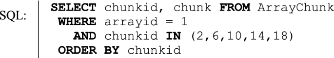

This would work well until the SQL query size limit is reached.
IN (buffered): an obvious workaround is to buffer the chunk ids (and the description of associated data copying to be performed), and send a series of queries containing limited-size IN lists.
SPD (sequence pattern detection): sending a query like
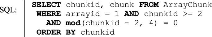

Here the condition expresses a certain cyclic pattern. Such a pattern is described by origin (2 in the example above), divisor (4 in the example above), storing the total periodicity of repetitions, and the modulus list (consisting of single 0 in the example above), containing the repeated offsets. The size or complexity of a pattern is the length of its modulus list. Section 5 describes our algorithm for detecting such patterns.
While most cases the SPD strategy will allow us to send a single query retrieving all desired chunks. If the pattern was too complex to be inferred from the buffer (e.g. there was no cyclic pattern at all), some extra chunks might also be retrieved. Still, there are two problems with a straightforward application of SPD: (1) in cases when there actually is a cyclic pattern it is unnecessary to identify all the relevant chunk ids first—a small sample list of chunk ids is normally enough; and (2) in case of an acyclic (random) access, like query QT6 defined in Sect. 6, the detected pattern might be as long as the list of chunk ids, thus making it a similar problem as for IN (single). Hence two versions of SPD:
SPD (buffered): solving the two above problems by computing a small sample sequence of the needed chunk ids, and then formulating and sending an SQL query with the detected pattern. If the pattern covers all the chunks to be retrieved, the single SQL query does all the work. Otherwise (on the first false-negative, or when the false-positives limit is reached), the SQL query is stopped and the buffering process is restarted. In the worst case (when there is no cyclic pattern), it will work similarly to IN (buffered), otherwise, fewer queries will be needed to return the same set of chunks.
SPD-IN (buffered): the difference between IN and SPD-generated SQL queries is that in IN, the chunkid values are explicitly bound to a list, which allows most RDBMSs to utilize the (arrayid, chunkid) composite index directly. As we have discovered in our experiments, neither MS SQL Server nor MySQL are utilizing an index when processing a query with mod condition.
However, by comparing a pattern size (i.e. length of the modulus list) to the number of distinct chunk ids in the buffer, we can easily identify if a realistic pattern was really discovered, or should we generate an IN query instead. We currently use the following rules to switch between IN and SPD buffer-to-SQL query translations:
- (A)
If the pattern size is less than half the number of distinct chunk ids, then the cycle is not completely repeated, and is probably not detected at all.
- (B)
If the sample size is less than the buffer limit—then we have buffered the last chunk ids for the query, so there is no advantage of using SPD either.
5 Sequence pattern detector (SPD) algorithm
Once the buffer is filled with chunk ids, an SQL query needs to be generated based on the buffer contents. An IN query is simple to generate, and the list of chunk ids does not even need to be sorted (the RDBMS performs this sorting if using a clustered index). In order to generate an SPD query, we first extract and sort the list of distinct chunk ids from the buffer.
The following algorithm operates on an increasing sequence of numbers—in our case—sorted chunk ids. Since we are detecting a cyclic pattern, we are not interested in the absolute values of the ids in the sequence, we will only store the first id as the point of origin, and the input values to the algorithm are the positive deltas between the subsequent chunk ids.
Each input is processed as a separate step, as shown in Fig. 2. The state of the algorithm is stored with the history and pattern lists, (initialized empty), and the next pointer into the pattern list (initialized to an invalid pointer which will fail any comparison operation).

A step in the SPD algorithm
The general idea is that each input either conforms to the existing pattern or not. In the latter case the second guess for the pattern is the history of all inputs. The input either conforms to that new pattern, or the new pattern (which is now equal to history) is extended with the new input. In either case, input is appended to history, and count is incremented.
The resulting pattern will have the form:
where x is the chunk id value to retrieve, x0 is the first chunk id value generated (i.e. ‘reference point’), d is the divisor, and m1,…,mn−1 is the modulus list. The generated pattern is the sequence of offsets P = <p1,…,pn>. We will compute the divisor as the total offset in the pattern, and each element in the modulus list is the partial sum of offsets:
In the next section we compare this strategy of formulating an SQL query with the more straightforward approach of sending IN lists that was presented in Sect. 4.
6 Comparing the storage and retrieval strategies
For evaluation of the different storage approaches and query processing strategies we use synthetic data and query templates for the different access patterns where parameters control the selectivity. The synthetic arrays are populated with random values, as data access performance is independent of these.
For simplicity and ease of validation, we use two-dimensional square arrays throughout our experiments. More complex access patterns may arise when answering similar queries to arrays of larger dimensionality. Still, as shown below, the two-dimensional case already provides a wide spectrum of access patterns, sufficient to evaluate and compare our array storage alternatives and query processing strategies. We use parameterized SciSPARQL queries, which are listed in Table 2, for our experiments. The queries involve typical access patterns, such as: accessing elements from one or several rows, one or several columns, in diagonal bands, randomly, or in random clusters.
The efficiency of query processing thus can be evaluated as a function of parameters from four different categories: data properties, data storage options, query properties, and query processing options, as summarized in Table 1. A plus sign indicates that multiple choices were compared during an experiment, and a dot sign corresponds to a fixed choice.
The structure of the data remains the same throughout the experiments. Namely, it is the dataset shown on Fig. 1, containing a single 100,000 × 100,000 array of integer (4-byte) elements, with total size ~ 40 GB. The logical nesting order is also fixed as row-major, changing it would effectively swap row query QT1 and column query QT2 while having no impact on the other query types from Table 2. The rest of the axes are explored during our experiments, as Table 1 indicates.
Experiment 1 compares the performance of different query processing strategies (including different buffer sizes), as introduced in Sect. 4, for different kinds of queries. For each kind of query, cases of different selectivity are compared under either data partitioning approach.
Experiment 2 explores the influence of chunk size on the query performance. There is obviously a trade-off between retrieving too much irrelevant data (when the chunks are big) and forcing the back-end to perform too many lookups in a chunk table (when the chunks are small).
For both experiments, the selectivity is shown both as the number of array elements accessed and the number of the relevant chunks retrieved. Our expectations that the latter quantity has higher impact on overall query response time are confirmed.
The experiments were run with our SciSPARQL prototype and the back-end MS SQL Server 2008 R2 deployed on the same HP Compaq 8100 workstation with Intel Core i5 CPU @ 2.80 GHz, 8 GB RAM and running Windows Server 2008 R2 Standard SP1. The communication was done via MS SQL JDBC Driver version 4.1 available from Microsoft.
6.1 Query generator
Similarly to the examples above, in each query template we identify an array-valued triple directly by its subject and property, thus including a single SPARQL triple pattern:

Each time we retrieve a certain subset of an array and return it either as a single small array (QT1–QT3) or the single elements accompanied by their subscript values (other queries). The templates listed in Table 2 differ only in the array access involved, with conditions on variables for array subscripts.
For the random access patterns, the main parameters are the random array subscripts. Nodes of type :AccessIdx with :i and ?j properties are added into the RDF dataset. Both data and query generators are part of the SciPARQL project, and are available at the project homepage [9].
6.2 Experiment 1: Comparing the retrieval strategies
We compare the different query processing strategies and the impact of buffer sizes for each query presented in Table 2, with different parameter cases resulting in the varying selectivity (and, in case of QT3, logical locality). Each query and parameter case is run against two stored instances of the dataset, differing in array partitioning method:
Linear chunks The array is stored in row-major order, in chunks of 40,000 bytes (10 chunks per row, 10,000 elements per chunk, 1,000,000 chunks total) using linear partitioning.
Square tiles The array is stored in 100 × 100 tiles, occupying 40,000 bytes each (10,000 elements per tile, 1,000,000 tiles total—same as above) using multidimensional partitioning.
We pick the strategies among the buffered variants of SPD, IN, SPD-IN, as described in Sect. 4. The buffer size is also varied for the IN strategy, with values picked among 16, 256, and 4096 distinct chunk ids. The SPD strategy is not affected by the buffer size in our cases—it either discovers the cyclic pattern with the buffer size of 16 or does not. We will refer to the SQL queries generated according to either SPD (buffered) or SPD-IN strategy described in Sect. 4 as SPDqueries, and similarly, to the SQL queries generated according to IN (buffered) or SPD-IN strategy as INqueries.
The query parameters are chosen manually, to ensure different selectivity (for all query patterns) and absence of data overlap between the parameter cases (for QT1–QT3). The latter is important to minimize the impact of the back-end DBMS-side caching of SQL query results. A set of chosen parameter values for a SciSPARQL query will be referred to as a parameter case. Each query for each parameter case is repeated 5 times, and the average time among the last 4 repetitions is used for comparison.
6.2.1 Results and immediate conclusions
The performance measurements are summarized in Table 3 below. For each query and parameter case, we indicate the amount of array elements accessed, and averaged query response times for different strategies. Chunk/tile access numbers shown with * are slightly greater for SPD and SPD-IN strategies due to false positives, with **—also differ for IN strategies due to advantages of sorting, shown for IN(4096). Here are the immediate observations for each query pattern.
QT1: The SPD strategy becomes slightly better than IN(4096) in a situation of extremely good physical locality (retrieving every chunk among the first 0.1% of the chunks in the database). Under more sparse access, IN with a big enough buffer, also sending a single SQL query, is preferable.
QT2: Worst case workload for the linear partitioning, given the row-major nesting order. As expected, the performance is roughly the same as for QT1 in the case of multidimensional partitioning, with the same maximum of 1000 square tiles being retrieved (this time, making up for one column of tiles). The long and sparse range of rows, given by QT2 access pattern, thus incurs slower-than-indexSPD performance (e.g. slower than the index lookups used by IN strategies). In contrast a short condensed range (as for QT1) is faster-than-index—as a non-selective scan is generally faster than index lookups.
QT3: In the case of multidimensional array partitioning and under certain grid densities, this query becomes a worst case workload—retrieving a single element from every tile. The IN strategy with a large buffer is the best choice in all cases, regardless of the partitioning scheme.
QT4: Similarly to query QT2, this one is the worst case workload for linear chunk partitioning, as the chunk access pattern, as detected by SPD changes along the diagonal, is initiating re-buffering and cyclic phase switching in our framework. The SPD strategy sends only 10 SQL queries (or a single query in case of b = 1000, where it captures the complexity of the whole pattern with a single access pattern), and SPD-IN always chooses SPD. Multidimensional partitioning helps to avoid worst cases for diagonal queries, helping to speed up the execution by factor of 55.4 (for the unselective queries).
QT5:SPD obviously detects wrong patterns (since there are no patterns to detect), leading to a serious slowdown. However, SPD-IN is able to discard most (but not all) of these patterns as unlikely, almost restoring the default IN performance. And, by the way, SPD is sending the same amount of 625 SQL queries as IN strategy does (for the buffer size of 16). Since the distribution is uniform, there is practically no difference between chunked and tiled partitioning,
QT6: The access coordinates are generated in clusters. For the test purposes we generate 3 clusters, with centroids uniformly distributed inside the matrix space. The probability of a sample being assigned to the cluster is uniform. Samples are normally distributed around the centroids with variance 0.01*N–0.03*N (randomly picked for each cluster once). We deliberately use such highly dispersed clusters, as the effects of logical locality already become visible at a certain selectivity threshold. Samples produced outside the NxN rectangle are discarded, thus effectively decreasing the weight of clusters with centroids close to the border.
For QT6, the effect of logical locality starts to play a role already when selecting 0.001% of the array elements. At the selectivity of 0.01% the number of chunks to access is just 78% to the number of elements in the case of linear chunks, and 69% in case of square tiles. We see that the square tiles better preserve the logical query locality, especially for the unselective queries. We expect this effect to be even greater for more compact clusters w.r.t. the tile size, and Experiment 2 below (where we vary the chunk size) supports this idea.
6.2.2 Comparing linear chunks versus square tiles
In this experiment we have gathered empirical proof to a common intuition [13, 20, 21, 24, 25] that for every data partitioning scheme there is a possible worst-case and well as best-case workload. These can be summarized by the following table, listing QT1–QT6 as representative access patterns (Table 4).
The multidimensional partitioning has its only worst case (when a separate chunk needs to be retrieved for each element) on sparse enough regular grids, Also, as shown by QT6, the multidimensional partitioning is still more advantageous for random access patterns, with even a small degree of locality. Overall, it can be regarded as more robust, though having fewer best-case matches. Compact enough clusters that can be spanned by a small number of tiles would obviously be a near-best-case access pattern.
6.2.3 Comparing SPD versus IN strategies
The SPD approach in most cases allows packing the sequence of all relevant chunk ids into a single SQL query, and thus skipping all the subsequent buffering. However, we have discovered that the SPD queries generally do not perform so well in the back-end DBMS as queries with IN lists. The last two cases show very clearly that in the case where there is no pattern, so that we have to send the same amount of SPD and IN queries (for the same buffer size), the difference in query response time is greater than order of magnitude.
An obvious explanation to this is index utilization. A query with an IN list involves index lookups for each chunk id in the list, while a query with mod condition, as generated with SPD strategy, is processed straightforwardly as a scan through the whole ArrayChunk table.
We believe it could be highly advantageous to implement a simple rewrite on the mod() function. A condition like ‘X mod Y = Z’ with Z and Y known, and X being an attribute in a table (and thus having a finite set of possible bindings), could be easily rewritten to generate a sequence of possible X values on the fly (thus making mod() effectively a multidirectional function [26]).
This, however, would require a facility to generate non-materialized sequences in the execution plan. In our prototype generators are used for all bag-valued functions. We have run additional experiments with other RDBMSs, including PostgreSQL, MySQL, Mimer [27], and found that even though some of these support table-valued UDF, only the newer versions (tested 9.4.4) of PostgreSQL are capable of avoiding materialization of complete sequences before use. We see this as an important improvement in the present-day RDBMS architecture.
6.3 Experiment 2: Varying the chunk size
Here we evaluate the trade-off between the need to retrieve many small chunks in one extreme case, and few big chunks (with mostly irrelevant data) in the other extreme case. We chose QT6 as a query with certain degree of spatial locality especially with tiled array partitioning.
We also study how well our back-end DBMS handles the requests for numerous small or big binary values, thus using the IN strategy with buffer size set to 4096 distinct chunks. In each case we retrieve 10,000 array elements arranged into three clusters, with variance chosen in range 0.01*N… 0.03*N.
Table 5 shows the results for both partitioning cases: even though big chunk size (around 4 megabytes) results in a much smaller amount of chunks retrieved (only 1 SQL query is sent), the overall query time rises super-linearly to 612 s. Besides that, smaller chunks result in slightly better performance in this case, since the amount of ‘small’ chunks retrieved stays approximately the same for the same sparse random access.
Using the square tiles helps to leverage the access locality even better. However, big tiles do not seem to pay off at this level of sparsity: retrieving 206 4-megabyte tiles results in a factor of 81.4 larger binary data retrieval than 9886 1-kilobyte tiles, and contributes to a factor of 9.26 longer query time.
This experiment shows that for the given access selectivity (10−6 of the total number of array elements selected randomly in clusters), small chunks perform better than big chunks, and the choice between linear chunks or square tiles is not important for small chunk/tile sizes. However, there is apparently a significant overhead in retrieving separate chunks, as a factor of 81.4 gross data transfer increase contributes to only a factor of 9.26 query time increase.
Analytically, we would model the query response time as a function T(s) of chunk size s: T(s)= P(s)N(s) where P(s) is the cost of transferring one chunk (given a fixed total number of SQL calls), and N(s) is the amount of relevant chunks to be retrieved. We expect P(s) to be linear after some ‘efficient chunk size’ threshold, while N(s) should experience a steep fall, corresponding to the logical locality of the query, which is saturated at some point. While the quantitative properties of P(s) depend largely on the underlying DBMS, the middleware, and the operating system used (along with hardware configurations), N(s) is statistical, and can be easily computed by simulation, as presented below.
6.3.1 Amount of distinct chunks as a function of chunk size
Figures 3, 4 and 5 below show the simulation results of QT6 retrieving 10,000 random elements, with clusters of element coordinates having the average variance of 0.2*N (very dispersed) to 0.0002*N (very condensed). Figure 3 presents N(s), given the linear chunks of varying size, and Figs. 4, 5 present N(s) for the square tiles.

Amount of distinct linear chunks as a function of chunk size, results of simulating QT6 retrieving 10,000 elements clustered with different density

Amount of distinct square tiles as a function of tile size, results of simulating QT6 retrieving 10,000 elements clustered with different density

Amount of distinct square tiles as a function of tile size, results of simulating QT6 retrieving 1000 elements clustered with different density
As we can see, the linear chunk case clearly exhibits a top ‘plateau’ for most of our cases, and thus confirms our expectations stated above. This feature is not visible for the square tiles case (Fig. 4), as the square tiles utilize the query locality much better. In order to see the plateau, we have to re-run the simulation with a greater sparsity (so that there is a greater probability of having single selected element per tile retrieved). Figure 5 shows the result of such simulation, with QT6 retrieving this time only 1000 random elements.
Another interesting feature on Figs. 3 and 5 is a ‘middle plateau’ for the (not very) dispersed access patterns. The beginning of such plateau should be considered as one of the sweet spots when choosing the partitioning granularity, where chunk/tile size is adequate to the distribution of access densities. Of course, assuming the statistical properties of the workload are known before the array data is partitioned.
Similarly, the earlier observations (Table 5) suggest that there is always a threshold in access density after which the bigger chunks become more favorable. We estimate it pays off to transfer 8 times more gross data from a back-end, if it results in retrieving 8 times lesser amount of chunks.
7 Summary
We have presented a framework for answering array queries, which identifies and makes use of the array access patterns found in those queries. We have implemented this approach in our software prototype supporting array query language (SciSPARQL) and storing numeric arrays externally. Buffering array access operations and formulating aggregated queries to the back-end has proven to be essential for performance.
We have compared two pure and one hybrid strategy for generating SQL queries to the back-end based on the buffered set of chunk ids to be retrieved. One is putting a long IN list into the query, and the other is creating an expression for a cyclic chunk access pattern discovered. It turned out that even though the second approach allows accessing an entire array with a single SQL query, and skipping further buffering in most cases; it only pays off for very unselective queries, retrieving a large percentage of array’s chunks. Apparently, current RDBMS optimization algorithms do not rewrite the kind of conditional expressions we were using, in order to utilize existing indexes. Hence, our general advice is to use long IN lists for the best performance of a contemporary RDBMS as a back-end.
We have also investigated two distinct partitioning schemes—linear and multidimensional—used to store large numeric arrays as binary objects in a relational database back-end. Our mini-benchmark consists of six distinct parameterized query patterns, and it becomes clear that for each partitioning scheme one can easily define best-case and worst-case queries. For example, a diagonal access pattern works much better with square tiles than with any linear chunking, while the linear chunks in an array stored row-by-row are perfect for single-row queries and worst for single-column queries. As for the chunk size, we have empirically found a proportion when the overhead of transferring more gross data balances out the overhead of retrieving more chunks.
The conclusion is that choosing the right partitioning scheme and chunk size is crucial for array query response time, and the choices being made should be workload-aware whenever possible. Though it might not be possible to know the expected workload for long-term storage of scientific data, such knowledge can certainly be inferred for materializations of intermediate results in cascading array computation tasks. As one direction of the future work, a query optimizer that makes choices on materializing intermediate results (e.g. common array subexpressions) should be enabled to choose the storage options based on the downstream operations, guided by the results of this study.
References
Hey T, Tansley S, Tolle K (eds) (2009) The fourth paradigm: data-intensive scientific discovery. ISBN 978-0-9825442-0-4, Microsoft Research
Misev D, Baumann P (2014). Extending the SQL array concept to support scientific analytics. In: Proceedings of 26th international conference on scientific and statistical database management (SSDBM), Aalborg, Denmark
SPARQL 1.1 Query Language. http://www.w3.org/TR/sparql11-query/. Accessed 27 Mar 2020
Andrejev A, Risch T (2012) Scientific SPARQL: semantic web queries over scientific data. In: Proceedings of third international workshop on data engineering meets the semantic web (DESWEB), Washington DC, USA
Andrejev A, Toor S, Hellander A, Holmgren S, Risch T (2013) Scientific analysis by queries in extended SPARQL over a scalable e-Science data store. In: Proceedings of 9th IEEE international conference on e-Science, Beijing, China
Andrejev A, He X, Risch T (2014) Scientific data as RDF with arrays: tight integration of SciSPARQL queries into Matlab. In: Proceedings of 13th international semantic web conference (ISWC’14), Riva del Garda, Italy
Andrejev A, Misev D, Baumann P, Risch T (2015) Spatio-temporal gridded data processing on the semantic web. In: Proceedings of IEEE international conference on data science and data-intensive systems (DSDIS), Sydney, Australia
Andrejev A (2016) Semantic web queries over scientific data. ISSN 1104-2516, Uppsala Dissertations from the Faculty of Science and Technology 121, Acta Universitatis Upsaliensis
Scientific SPARQL. http://www.it.uu.se/research/group/udbl/SciSPARQL/. Accessed 27 Mar 2020
Kersten M, Zhang Y, Ivanova M, Nes N (2011) SciQL, a query language for science applications. In: Proceedings of EDBT/ICDT workshop on array databases, Uppsala, Sweden
van Ballegooij A, Cornacchia R (2005) Distribution rules for array database queries. In: Proceedings of 16th international conference on database and expert systems applications (DEXA), Copenhagen, Denmark
RDF Data Cube. http://www.w3.org/TR/vocab-data-cube/. Accessed 27 Mar 2020
Sarawagi S, Stonebraker M (1994) Efficient organization of large multidimensional arrarys. In: Proceedings of 10th IEEE international conference on data engineering (ICDE’94), Houston TX, USA
Baumann P (1994) On the management of multidimensional discrete data. VLDB J 4(3):401–444 (Special Issue on Spatial Database Systems)
Dobos L, Szalay A, Blakeley J, Budavári T, Csabai I, Tomic D, Milovanovic M, Tintor M, Jovanovic A (2011) Array requirements for scientific applications and an implementation for microsoft SQL server. In: Proceedings of EDBT/ICDT workshop on array databases, Uppsala, Sweden
NetCDF. http://www.unidata.ucar.edu/software/netcdf/. Accessed 27 Mar 2020
Brun R, Rademakers F (1997) ROOT—an object oriented data analysis framework. Nucl Instrum Methods Phys Res, Sect A 389(1–2):81–86
Buck JB, Watkins N, LeFevre J, Ioannidou K, Maltzahn C, Polyzotis N, Brandt S (2011) SciHadoop: array-based query processing in hadoop. In: SC ‘11: proceedings of 2011 international conference for high performance computing, networking, storage and analysis
Brown PG (2010) Overview of SciDB: large scale array storage, processing and analysis. In: Proceedings 2010 ACM SIGMOD/PODS conference, Indianapolis IN, USA
Furtado P, Baumann P (1999) Storage of multidimensional arrays based on arbitrary tiling. In: Proceedings of 15th IEEE international conference on data engineering (ICDE’99), Sydney, Australia
Marques P, Furtado P, Baumann P (1998) An efficient strategy for tiling multidimensional OLAP data cubes. In: Proceedings workshop on data mining and data warehousing (Informatik’98), Magdeburg, Germany
Soroush E, Balazinska M, Wang DL (2011) Arraystore: a storage manager for complex parallel array processing. In: Proceedings of. ACM SIGMOD/PODS conference. Athens, Greece
Zhang Y, Munagala K, Yang J (2011) Storing matrices on disk: theory and practice revisited. Proc VLDB Endow 4(11):1075–1086
Wang Y, Nandi A, Agrawal G (2014) SAGA: array storage as a DB with support for structural aggregations. In: Proceedings of 26th international conference on scientific and statistical database management (SSDBM), Aalborg, Denmark
Cohen J, Dolan B, Dunlap M, Hellerstein JM, Weltonl C (2009) MAD skills: new analysis practices for big data. In: Proceedings of 35th international conference on very large data bases (VLDB’09), Lyon, France
Flodin S, Orsborn K, Risch T (1998) Using queries with multi-directional functions for numerical database applications. In: Proceedings of 2nd East-European symposium on advances in databases and information systems (ADBIS’98), Poznan, Poland
Mimer SQL. http://www.mimer.com. Accessed 27 Mar 2020
Acknowledgements
Open access funding provided by Uppsala University. This project is supported by eSSENCE and the Swedish Foundation for Strategic Research, Grant RIT08-0041.
Author information
Authors and Affiliations
Corresponding author
Additional information
Publisher's Note
Springer Nature remains neutral with regard to jurisdictional claims in published maps and institutional affiliations.
Rights and permissions
Open Access This article is licensed under a Creative Commons Attribution 4.0 International License, which permits use, sharing, adaptation, distribution and reproduction in any medium or format, as long as you give appropriate credit to the original author(s) and the source, provide a link to the Creative Commons licence, and indicate if changes were made. The images or other third party material in this article are included in the article's Creative Commons licence, unless indicated otherwise in a credit line to the material. If material is not included in the article's Creative Commons licence and your intended use is not permitted by statutory regulation or exceeds the permitted use, you will need to obtain permission directly from the copyright holder. To view a copy of this licence, visit http://creativecommons.org/licenses/by/4.0/.
About this article

Cite this article
Andrejev, A., Orsborn, K. & Risch, T. Strategies for array data retrieval from a relational back-end based on access patterns. Computing 102, 1139–1158 (2020). https://doi.org/10.1007/s00607-020-00804-x
Received:
Accepted:
Published:
Issue Date:
DOI: https://doi.org/10.1007/s00607-020-00804-x