Seemingly Unrelated Mixed-Effects Biomass Models for Young Silver Birch Stands on Post-Agricultural Lands

1
Institute of Forest Sciences, Warsaw University of Life Sciences-SGGW, Nowoursynowska 159, PL 02-776 Warsaw, Poland
2
School of Computing, University of Eastern Finland, P.O. Box 111, FI-80101 Joensuu, Finland
*
Author to whom correspondence should be addressed.
Forests 2020, 11(4), 381; https://doi.org/10.3390/f11040381
Submission received: 27 February 2020
/
Revised: 23 March 2020
/
Accepted: 25 March 2020
/
Published: 27 March 2020
(This article belongs to the Special Issue Modelling of Forests Structure and Biomass Distribution)
Abstract
:Secondary succession that occurs on abandoned farmlands is an important source of biomass carbon stocks. Both direct and indirect tree biomass estimation methods are applied on forest lands. Using empirical data from 148 uprooted trees, we developed a seemingly unrelated mixed-effects models system for the young silver birch that grows on post agricultural lands in central Poland. Tree height, biomass of stem, branches, foliage, and roots are used as dependent variables; the diameter at breast height is used as the independent variable. During model elaboration we used restricted cubic spline: 5 knots at the quantiles (0.05, 0.275, 0.5, 0.725, and 0.95) of diameter at breast height provided sufficiently flexible curves for all biomass components. In this study, we demonstrate the use of the model system through cross-model calibration of the biomass component model using tree height measured from 0, 2, 3, and 4 available extreme trees feature in the plot in question. A different number of extreme trees were measured for final model system and our results indicated that for all analyzed components, random-effect predictions are characterized by higher accuracy than fixed-effects predictions.
1. Introduction
Issues related to climate change have become increasingly important, as evidenced by the world’s strongest climate-energy policy agreed upon by the European Council in October 2014. The policy’s objective assumes that within the European Union (EU): (i) at least 32% of the energy demand is being covered by renewable energy sources and (ii) greenhouse gas emissions (from 1990 levels) will be cut by 40% by 2030. In this context, due to the area occupied and the amount of accumulated carbon, forest ecosystems play an important role. For example, the content of carbon in biomass of Polish forests has been estimated at 822 million tons [1]. It is worth noting, however, that due to the difficulty of defining the current method of land management, almost 800 thousand ha of forests are not included in the official statistics [2]. One of the types of land that is not covered by official statistics is secondary succession, which occurs on abandoned farmlands and are an important source of biomass carbon stocks [3,4,5]. These areas are frequently subjected to appearance of pioneer forest tree species, such as silver birch (Betula pendula Roth.) [6,7]. Those stands during the first eight years produce 31.2 Mg/ha aboveground biomass [7] and after 15 years can produce up to 75 tons Mg/ha [8]. By introducing rapid rotation in these areas, it is possible to increase the potential of fast growing silver birch stands, which can be assessed using a life cycle analysis [9].
Biomass conversion and expansion factors, combined with stand level volume, are an exemplary approach to estimating forest biomass stock [10,11,12]. Allometric biomass models are also a common solution. In this option, total biomass and/or biomass of each tree component is expressed as a function of tree-level predictors, such as diameter at breast height [13], only diameter at breast height [14,15], diameter at ground level [16], only tree height [17], or diameter at ground level and tree height [18]. Regardless of the type of predictor, field measurements are a common source of modelling data. An example of such a solution are aboveground biomass functions derived for birch in Norway [19]. In Finland, Mälkönen [20] analyzed the total aboveground biomass production in 40-year-old silver birch stands. Johansson [21] elaborated biomass equations for silver birch stands growing on abandoned farmland in Sweden. Kuznetsova et al. [16] performed similar studies in Estonia. In Poland, Bronisz et al. [22] estimated allometric empirical biomass models for total aboveground, stem, branches, and foliage dry biomass. However, for the estimating of net primary production, biomass allocation, belowground competition, and carbon accumulation quantifying belowground biomass is crucial [23,24,25].
When formulating a model for the total above/belowground biomass of trees and their components, it is important to ensure that the logical assumption is made that the sum of the components of the tree estimated using equations should be equal to the estimated biomass of the whole tree additivity of biomass models. Threads regarding the use of seemingly unrelated regression (SUR) to obtain biomass model additivity was raised by Kozak [26], discussed by Chiyenda and Kozak [27], and by Cunia and Briggs [28]. Parresol [29] pointed out three possible procedures during SUR elaboration. In one of them, the total biomass regression model is defined as the sum of the individually calculated best regression models of the biomass of its components (equation 20 in [29]) and the joint behavior of the separate components is modeled through cross-model correlation. Therefore, SUR has been increasingly used to develop various additive biomass models. However, we point out that the additivity is not ensured through the SUR estimation method, but through such formulation of the model equations that the system is compatible. Bi et al. [30] applied this solution for biomass modeling of 15 native eucalypt forest tree species in temperate Australia. While Dong et al. [31] developed additive biomass equations for three coniferous plantation species in Northeast China, Lambert et al. [32] elaborated new sets of Canadian national tree aboveground biomass equations. Examples of European research are biomass models developed for the main hardwood forest species in Spain [33] or Polish research related to Scots Pine [34] or Silver birch [22] aboveground biomass modeling.
The data for biomass models is often characterized by a grouped structure. It usually contains information about individual tree features for different sample plots. Moreover, the relationship between independent variables (e.g., diameter at breast height/height) and biomass components as dependent ones varies among different sample plots. The mixed-effects models, where the fixed and random-effects are distinguished, is useful solution in those types of forestry data set [35]. The fixed part of those models allows modelling data for a typical sample plot. A random part describes the difference of each plot and the typical plot, thus enabling description of the plot specific relationship for all plots of the dataset [36]. In addition, it allows for a significant improvement of biomass meta-models for local conditions [37]. Mixed-effect models approach allows to include various data structures through inclusion of random effects at different levels of grouping, it can be based on country or region [38]. Mixed-effect biomass models are analyzed in different forms. Ou et al. [39] for example defined nonlinear mixed-effects models for aboveground biomass of natural Simao pine in Yunnan (China), whereas Fehrmann et al. [36] developed linear mixed-effects models for logarithmic biomass based on the national forest inventory of Finland’s forests. Furthermore Pearce et al. [40] defined linear mixed-effects models for estimating biomass and fuel loads in shrublands. A flexible but less frequently used solution in case of biomass modeling is the spline regression. Spline is a function consisting of pieces of second or third order polynomials that are joined at knots [41]. Those type of function remains as linear with respect to its parameters and the spline provides a way to calculate additional transformation of the variable. The function’s flexibility is controlled by the number of knots, which can be placed at certain quantiles of the independent variable [35].
One benefit from the mixed-effects model is the flexibility in prediction. If no local information to predict the random effects for the plot in question are available, a prediction using the fixed part of the model can be used. Using the fixed part of mixed-effects models provides predictions for a typical plot and in case of nonlinear models it could be biased [42]. However, if even a small amount of local measurements are available, a more accurate random-effect prediction can be used [43,44]. In the multivariate modeling context, such prediction utilizes the cross-model correlations of the model system, thus taking into account the logical interactions between the biomass components. Furthermore, those model systems allow use of the cross-model residuals correlation to predict residuals for all dependent variables for the calibration trees in question. Lappi [43] developed a bivariate system of seemingly unrelated mixed-effects model for tree height and volume, and used the system for prediction of standing tree volume both when measurements of tree height were not available and when they were available from the plot in question. In this study, we extend this idea to the multivariate system including models for biomass components and tree height. The model system allows prediction of plot-level biomass-diameter models and further improving that prediction using local measurements of tree heights from the plot in question. Above predictions is based on the estimated best linear unbiased predictor (EBLUP) and it utilizes the estimated variance-covariance structure of random effects and residuals in a way that leads to statistically optimal prediction [42].
Using empirical data from 148 uprooted trees, we developed a seemingly unrelated mixed-effects models system for the young silver birch stands growing on post agricultural lands in central Poland. Tree height, biomass of stem, branches, foliage, and roots are used as dependent variables while diameter at breast height are used as the independent variable. We demonstrate the use of the model system through cross-model calibration of the biomass component models using tree height.
2. Material and Methods
2.1. Study Sites
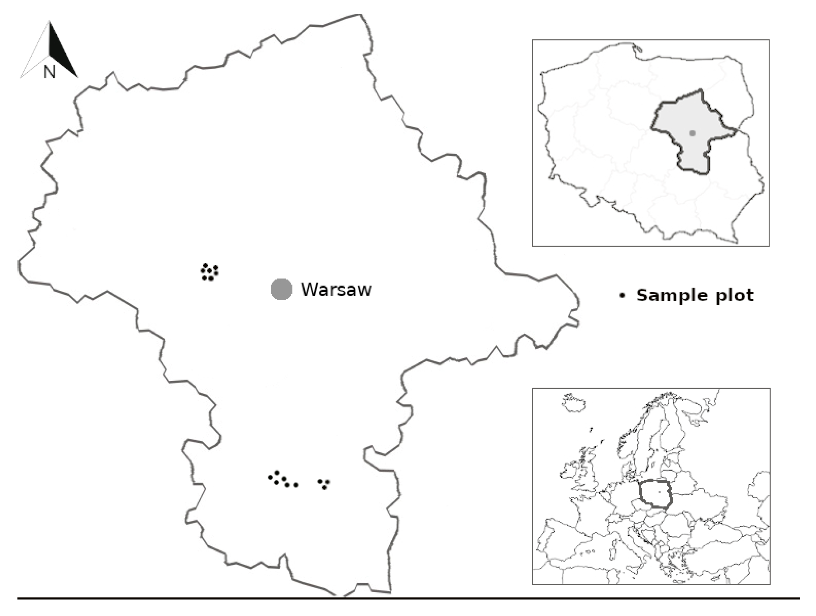
We used empirical data from 16 temporary sample plots located in silver birch stands growing on post-agricultural lands in Mazowieckie province, central Poland (52°21′–51°24′ N, 20°39′–21°26′ E, Figure 1). We analyzed stands originated from natural regeneration that started after farming use was stopped. No silvicultural treatments had been performed by the time the sample material was collected. All sample plots were located in a zone of transition from the maritime to continental type within the temperate climate [45]. Mean annual temperatures were in the range 6–8 °C. The average annual precipitation in the region amounted to 550–600 mm. Soils are generally poor in nutrients. Elevation ranged from 95 to 160 m above sea level. Each sample plot consisted of about 200 trees. We measured diameter at breast height of all living trees on sample plot. At each sample plot, we randomly chose ten trees from the range of diameters. For this study we selected trees taller than 1.3 m. Age of those trees varied from 3 to 16 years (Table 1).
2.2. Uprooted Trees
The sample trees were dug out with their root systems. We marked the base level at the bark prior to excavation to separate aboveground part of the tree from belowground one. We divided each tree into the following biomass components: stem, branches, foliage and roots (>2 mm of diameter according to [46]) separated from the stem at the previously marked base level.
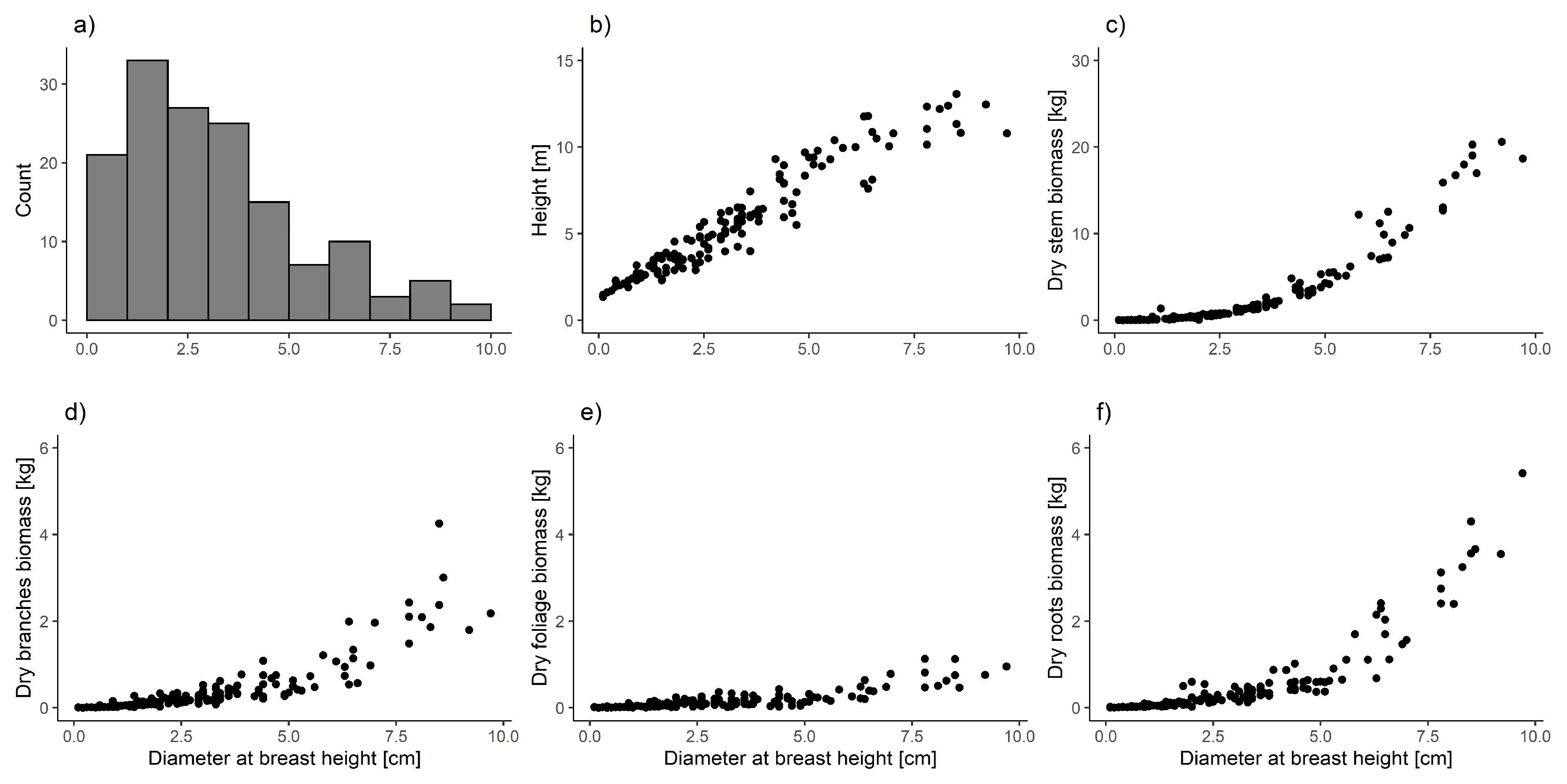
We cleared the roots from soil and other organic materials using brushed and compressed air. We weighted all biomass components in the field using precise portable scales (accuracy 0.01 g). We took samples of each component (stem discs in the middle of each 1 m section, random samples of branches, foliage, and roots) from every tree to calculate the ratio between fresh and dry biomass. We dried the samples at 105 °C [47] until they reached a constant weight. We calculated the dry biomass of each biomass component for each tree on the basis of corresponding fresh to dry biomass ratios [46]. Finally, empirical material consisted of the data from 148 trees taller than 1.3 m. Diameter at breast height of those trees varied from 0.1 to 9.7 cm (Table 1, Figure 2).
2.3. Separate Mixed-Effect Models
We started the analysis by modeling the relationship between the dependent variables and tree diameter separately for each biomass component using a liner mixed-effect model. In our data, sample plots defined a single grouping factor and no other potential factors of grouping were present. Each model for the tree j, j = 1, …, ni, of plot i, i = 1, …, M, was of form:
where is the fixed part and the random part. We assume that:
where are independent among plots and of the residual errors . Matrix is a positive definite variance-covariance matrix of random effects. The zero-mean residual errors were mutually independent, normal with variance.
where and δ are the estimated scale and shape parameters for the power function, respectively. The special case leads to homoscedastic residuals. Notice that our model includes only diameter at breast height (DBH) as a fixed predictor, therefore prediction does not require that e.g. measurement of tree height is available. However, our multivariate system allows also improved predictions by utilizing measurements of height as well.
To ensure that the predicted biomass components and tree heights are positive, logarithmic biomass and logarithm of height-1.3 was used as . However, the logarithmic biomasses were not linear with respect of DBH or its logarithm and we used a restricted cubic spline to model this curvilinearity. The following restricted cubic spline with K nodes , was used in the fixed part [41].
The predictors in the last K-2 terms are the truncated power basis functions of form:
where is zero when and otherwise. This solution allows us to define model, which is smooth and curvilinear with respect to DBH, but linear with respect to the regression coefficients; equation (5) provides a way to compute nonlinear transformations of DBH. Initial exploration of the data suggested random intercept and coefficient of diameter in all models, therefore the random effects of form: were used in all models.
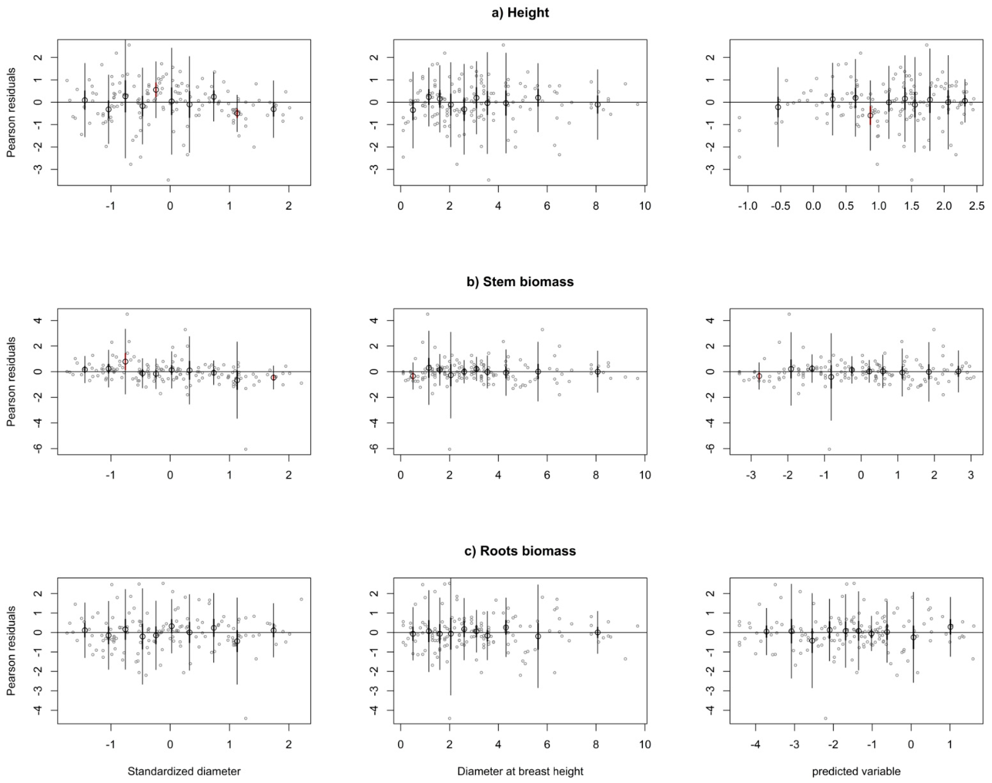
We used five knots placed at certain quantiles of the DBH following the suggestion of Harrell [41]. The number of knots was chosen based on the residuals behavior analysis and AIC (Akaike Information Criterion). Residual analysis for all dependent variables was carried out using plots of Pearson residuals in three variants: (i) the means of residuals in 10 classes of the standardized DBH were plotted together with the 95% confidence interval of individual observations (mean ± 1.96 SD) and the confidence interval for class mean (mean ± 1.96 SE). Standardized diameter was calculated as difference between individual tree diameter and mean diameter of the sample plot, divided by standard deviation of diameter in sample plot. The similar graphs were produced also (ii) in relation to DBH and (iii) the fitted values. Residuals were plotted as implemented in function mywhiskers of R-package lmfor [48].
2.4. Multivariate Seemingly Unrelated Mixed-Effects Model System
Multivariate (seemingly unrelated) mixed-effects models are seemingly unrelated models with random group effects. They are useful, in particular, when several independent variables are measured from the same sample units and the relationship among the random effects and residuals across models is of interest. Assume that we have L individual mixed-effects models and pool the observations of the mth response of plot i to vector and the corresponding model matrices of the fixed and random parts to and . The multivariate seemingly unrelated mixed-effects model system for each plot i, i = 1, …, m as [35]:
where for . We assume that the cross-model correlations of the random effects and residuals are the same for all groups. By defining and correspondingly for and (see [35] for details), the multivariate model can be written as univariate model:
where and are block-diagonal matrices, which have the response-specific model matrices on the diagonal. The variance-covariance matrix of the random effects is
and the correlation matrix of residual errors is
where are the cross-model covariances of random effects and is the correlation between the residual errors for the same tree between responses l and m. The variance-covariance matrix of residual errors is
where the diagonal matrix includes blocks for all responses l = 1, …, L, based on the variance functions of the univariate models. The cross-model covariance components of these matrices describe the joint behavior of group-specific functions and residual errors. Model (7) defined the multivariate model as a univariate linear mixed-effects model for a single plot. The definition of the model for whole data is straightforward. The parameter estimation was done using REML using R-package nlme. See [35] for more details about the model formulation and for an example about the implementation in R.
2.5. Fixed and Cross-Model Random-Effect Prediction
In general, mixed-effect models allows to use fixed-effect and random-effect prediction. Fixed-effect prediction assumes that the expected value of the random effects is 0 and it is optimal when no sample information about dependent variables are available from the plot in question. If measurements of even one tree are available from the plot in question, the random-effect prediction is justified. It may sound surprising that one measurements can be used for prediction of several parameters, but this is possible and justified because the approach uses the estimated variances within plots and between plots to optimally weight the fixed part of the model and the local measurements. The multivariate seemingly unrelated mixed-effects model allows to use also the cross-model correlations of random effects and residual errors to predict all dependent variables using measurements of some of them. Generally speaking, we can predict the random group effects for all dependent variables: both for the variables that have local measurements and for the variables that do not have local measurements for the plot in question [35]. We could also predict the residual errors of all response variables for the sampled trees [35,42].
Technically, we define vector y0 that includes from only those elements that have been observed. We define matrices D0 and R0 by removing from D and R those rows and columns that correspond to the unobserved variables. In addition, we define matrix C by removing from D all the columns that correspond to the unobserved variables but keeping all the rows, and Z0 and X0 by removing from Zi and Xi those rows and columns that correspond to the unobserved variables. The best linear predictor of the complete random effect vector for group i becomes [35]:
The prediction variance is
The fixed part and variance-covariance matrices are replaced by their estimates, which leads to EBLUP.
In our case, the heights and biomass components were predicted in a logarithmic scale. To transform them to the original scale we applied bias correction by adding half of the prediction variance into the predictions before applying the exponential transformation [35,49]. The required prediction variance was taken from the diagonal of . That variance ignores the components related to the estimation errors of fixed effects and variance-covariance components, but their effect is marginal because of the rather large data set.
In our case during plot-specific cross-model random–effect prediction we used tree height as the observed dependent variable that is used for calibration. We used a different number of available measured trees for prediction. The fixed-effect approach was applied for 0 available trees, whereas the cross-model random-effect prediction was created separately for 2, 3, and 4 available trees. From the literature of experimental design [50], we know the prediction error variance of a linear regression model is the lowest if the x-variables are taken from the endpoints of the range (extreme trees). Therefore, we used this procedure for cross-model random–effect prediction. We first randomly divided each sample plot, with 10 sample trees, into prediction and evaluation part. Afterwards, based on prediction part we conducted extreme trees sampling (2, 3, 4) for height measurement. We used DBH as the selection criterion as follows: 2 trees—the thinnest and the thickest tree; 3 trees—1 the thinnest and 2 the thickest trees; 4 trees—2 the thinnest and 2 the thickest trees. The sampling procedure was replicated 20 times for each plot. Based on trees forming the evaluation part of each sample plot and which were not used in calibration, we computed the root mean square error (RMSE). RMSE was calculated for each dependent variable as mean error achieved during all replication.
3. Results
Analysis of the residuals for individual models for each depended variable indicated the presence of heteroscedasticity. Therefore, we modeled the residual variance using a power function (3). The assumed variance function modeled the heteroscedasticity well (Figure 3). Likewise, a likelihood testing indicated that the variance function significantly improved the fit (p < 0.0001).
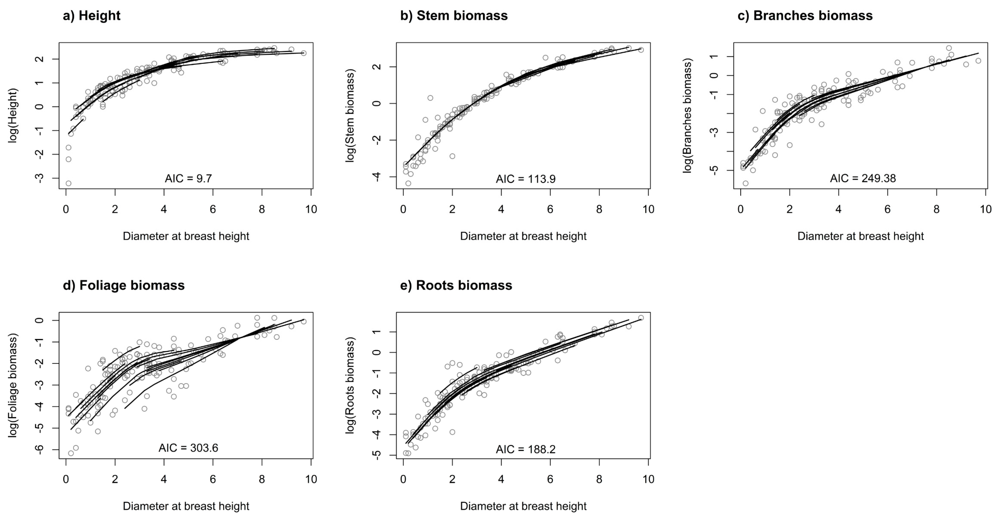
In the spline regression (4), we found that using five knots at the quantiles (0.05, 0.275, 0.5, 0.725, 0.95) of DBH provided sufficiently flexible curves for tree height and all analyzed biomass components (Figure 4).
Once the model form for the individual models was found, the model was fitted as a five-component seemingly unrelated mixed-effects model. The estimated regression coefficients and variance function parameters of the model system are given in Table 2.
The cross-model correlations of the random effects range from 0.08 to 0.995, being moderate or strong in most cases, which indicates that the cross-model calibration will be successful (Table 3). The random effects for height are most strongly correlated with random effects estimated for stem biomass. Considering the analyzed biomass components, it should be noted that the strongest relationship is observed between random effects achieved for foliage and branches biomass. Random effects for stem biomass, as component with the largest share in aboveground biomass, are strongly correlated with foliage and roots biomass. While random effects for roots biomass is strongly correlated with branches biomass.
Correlation between residual errors for analyzed dependent variables varies depending on the feature being assessed (Table 4). The strongest correlation is observed in the case of branches and foliage biomass. In addition, residual errors for roots biomass has a strong relationship to other aboveground biomass components. Residual error for tree height are not strongly correlated with biomass components—the highest in case of stem biomass.
Fixed and Cross-Model Random Effects Prediction
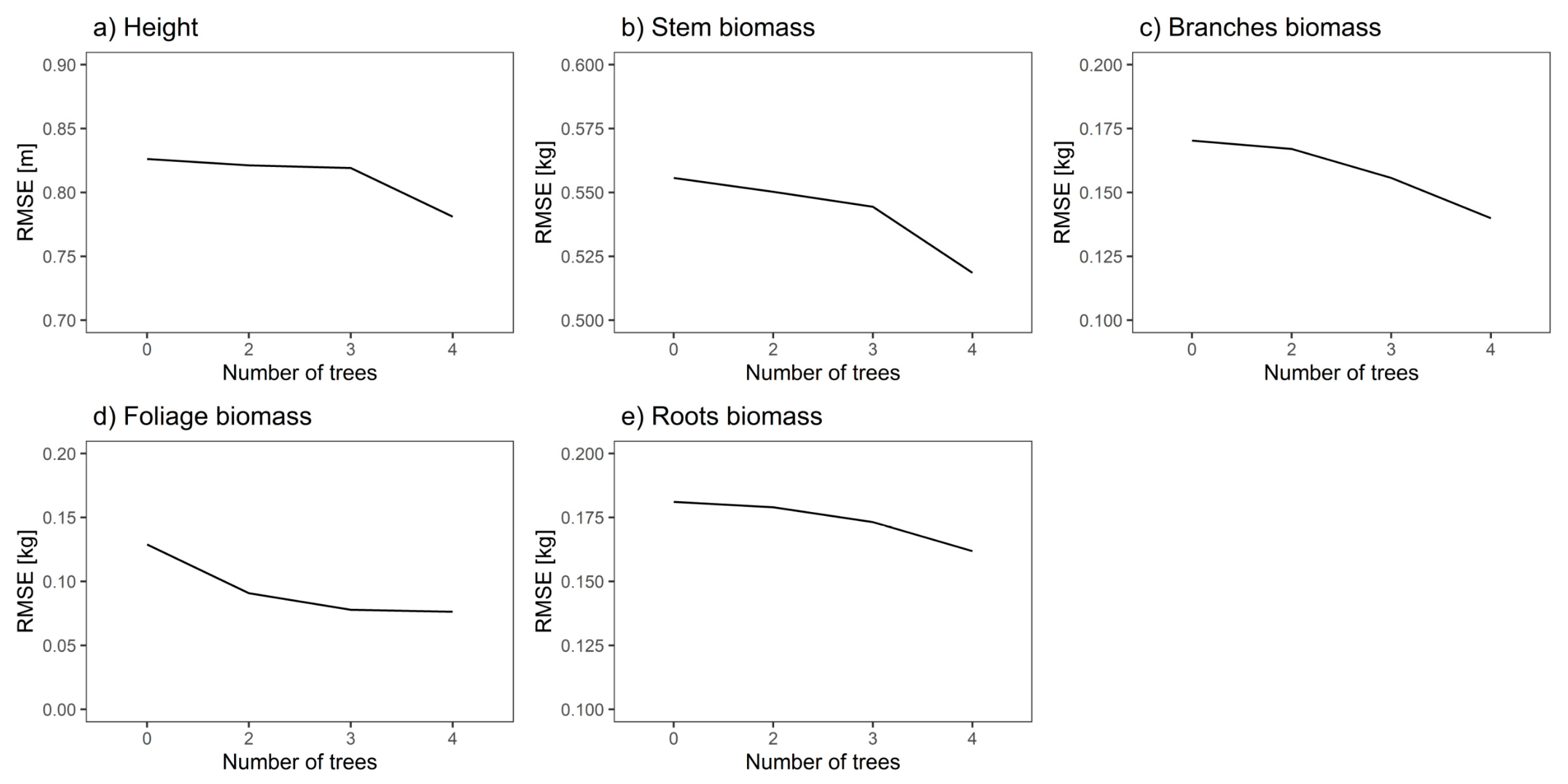
Applied different number of extreme trees measured for final model system indicated that for all analyzed depended variables random effects predictions have lower RMSE then fixed effects prediction, which serves as a reference in Figure 5 (Number of trees = 0). When the number of available trees is increased, the error decreases for all depended variables. The differences between RMSE values showed in Figure 5 would be clearer with more trees available. However, due to the limitations in the number of trees per plot of the data, we could not include more trees for random effect prediction.
In the case of height, using four trees in the random-effects prediction decreased the RMSE by 0.045 m (5.4%, Table 5) compared to the fixed-effect prediction. In case of biomass components the highest relative decrease was reached for foliage biomass and equals 41.1%, whereas the lowest relative difference occurs in case of stem biomass (6.7%; Table 5).
4. Discussion and Conclusions
In this study, based on 148 uprooted trees from 16 temporary sample plots, we developed a seemingly unrelated mixed-effects biomass model system for young silver birch stands growing on post agricultural lands in central Poland. We defined diameter at breast height as independent variable and tree height as well as the whole tree biomass components such as stem, branches, foliage, and roots biomass as dependent variables. During our analysis we applied fixed and random effect prediction. Under prediction we included the sample plot as the grouping level and tested height measurements for 2, 3, and 4 available trees in plot in question. It should be noted that the resulting model system is a solution with high potential in case of biomass modeling. On the one hand, it allows us to achieve information about roots biomass, which is difficult to measure, but is crucial according to the understanding and estimating carbon accumulation in birch forest ecosystems [8,23,24]. On the other hand, it potentially allows prediction of the tree-level residuals and therefore the use of either diameter or diameter and height in prediction of tree biomass using the procedures explained in Lappi [43] (see also [42]). Moreover, it allows us to take into account various data sources [55] and is a new voice in the discussion on biomass prediction using diameter at breast height and height [13,15]. In the context of potential use of achieved solution it is worth noting that during the cross-model random-effect prediction we focused on the trees available only for height measurements as the most accessible dependent variable. Therefore, taking into account the larger number of available trees and other dependent variables (such as measurements of stem biomass to improve the prediction of other biomass components) achieved model system will allow a broader understanding of accuracy of cross-model random–effect prediction.
In this study, we estimated total biomass as the sum of the individually calculated best regression models of the biomass of its components [29]. The variance is estimated by taking into account the cross-model covariances of random effects and residual errors. This approach was also used during creation of Canadian national aboveground biomass equations for six tree species [56]. However, they defined two types of models: (i) the DBH—based equations where, as in our case, DBH is an independent variable and (ii) the DBH—and height-based equations where, unlike in our study, the tree height was included as independent variable. Aboveground biomass additive models based on SUR were also created for the eight relevant tree species in Germany [57]. Likewise, Carvalho and Parresol [58] applied nonlinear seemingly unrelated regression (as nonlinear joint-generalized regression) for stem and crown biomass functions for Pyrenean oak trees in Portugal. Morever, in Poland, research was carried out taking into account SUR in biomass modeling. Zasada et al. [34] and Bronisz and Zasada [15] created additive biomass models for aboveground biomass of Scots Pine. While Bronisz et al. [22] focused on empirical equations for estimating aboveground biomass of silver birch. The aforementioned studies are examples of creating comprehensive solutions enabling biomass prediction of various tree components. In addition, these are solutions where DBH and height are defined as independent variables, while in our work we used a different approach which, to our knowledge, has not been previously used in biomass modeling. Parresol [59] formulated a system of biomass models where one of the components is the total biomass, which is just the sum of the other components of the system. Compatibility of predictions was ensured through parameter restrictions. However, even though the estimated variance of the total biomass in the empirical data set was lower, no theoretical arguments for the better performance of such an approach over the one we used was provided.
It is worth adding that model systems are not only used during biomass modeling. Fu et al. [60] indicates that seemingly unrelated regression allows to reach higher prediction accuracy for crown width than other methods such as adjustment in proportion or ordinary least square regression. Mehtätalo [61] created a model system for stand-specific diameter distribution while Siipilehto [62] developed a system of models for 20 stand-level variables (e.g., basal area, mean diameter and dominant height). Instead Maltamo et al. [55] predicted and calibrated diameter at breast height, tree height, volume, dead branch height and crown base height using airborne laser scanning.
Regardless of whether biomass is modeled using individual formulas or a model system, solutions based on linear regression are possible [63]. However, due to modeled biomass relationships, nonlinear regression is more often considered [21,22,25]. One of the reasons is that the biomass is always positive, which was in our case ensured by modeling logarithmic biomass. Another acceptable solution would be a generalized linear mixed-effect model based on gamma distribution [64]. During our study we modeled the curvilinear relationship of biomass and diameter by using a spline regression, which ensures that the model remains as linear. It is continuous function consisting of pieces of second or third order polynomials that are joined at knots [41]. In addition, Harrell [41] indicates that number of knots depends on the sample size. Others claim that for many datasets four knots offers a good enough fit of the model and is a compromise between flexibility and loss of precision caused by overfitting a small sample. Our results for individual mixed-effect models indicated that in the case of biomass modeling of young birch stable residual behavior and lowest AIC value is obtained for five knots. The results obtained in our study indicate that it is possible to use the spline function for biomass modeling based on empirical data. Splines have been used in biomass modeling previously in Bollandsås et al. [65]. During this research authors tested three approached for biomass estimation based on field and laser data collected in a mountain forest in southeastern Norway.
The data for biomass models is often characterized by a grouped structure. It usually contains information about individual tree biomass components for different sample plots. The relationship between variables varies among different sample plots. The resulting dependence is properly taken into account by using the mixed-effects models approach [66]. Smith et al. [25] in research on belowground and whole tree biomass of birch in Norway indicates that nonlinear mixed effects models approach for those type of modeling, with similar as in our case, single grouping factor is useful methodology for those type of modeling. The best model for whole tree biomass was evaluated using two independent variables (diameter at breast height and height). Repola [63] created three separate multivariate variance component linear models for aboveground and belowground biomass for birch trees in Finland. To reach homoscedasticity of the variance and to ensure positive biomasses, the author used logarithmic transformation of data. In our case, the logarithmic transformation did not lead to homoscedastic errors and an additional variance function was therefore used. As opposed to our approach, another author defined diameter at breast height and height as independent variables.
Linear mixed-effect models were also tested during the Fehrmann et al. [36] study. In their research, aboveground biomass was estimated for Finnish Scots pine and Norway spruce trees using three approaches: (i) k-nearest neighbour (k-NN), (ii) plot-specific linear mixed-effect biomass models, in which DBH and height were used as independent variables, and (iii) simple linear models. Based on the achieved results, they claimed that even fixed effect prediction based on linear mixed models allows for greater precision than an ordinary least squares regression.
In addition to taking into account the dependence structure caused by the grouping of the data, the mixed-effects modeling allows for the flexible prediction alternatives. In cases where in there is a lack of measurements, only fixed-effects can be used, yet additional measurements allow random-effects to be predicted [66]. Consequently, it allows for greater predictions accuracy in plots where additional measurements are available [44]. However, in the case of biomass modeling, obtaining additional measurements is troublesome because it is associated with the felling of trees. Multivariate mixed-effects model application allows to take full advantage of the mixed-effects models. In our case, additional measurements for tree height allows to reach more accurate random cross-model prediction for all analyzed biomass components. The same idea could be generalized also to root biomass: if measurements of the above-ground biomass components are available, our model would allow for (1) more accurate prediction for all biomass components of the plot and (2) even more accurate prediction of the root biomass for the sample trees through prediction of the residual error of that tree [42,43].
Author Contributions
K.B., conceptualization, software, investigation, resources, data curation, and writing—original draft. L.M., methodology, software, validation, writing—review and editing. All authors have read and agreed to the published version of the manuscript.
Funding
The research was financed by (i) the National Science Centre research grant “Ecological consequences of the silver birch (Betula pendula Roth.): Secondary succession on abandoned farmlands in central Poland” [grant no. N-N305-400238], (ii) Warsaw University of Life Sciences—SGGW scholarship fund, and (iii) Polish National Agency for Academic Exchange as part of the Foreign Promotion Program.
![Forests 11 00381 i001]()

Conflicts of Interest
The authors declare no conflict of interest.
References
- Raport o stanie lasów w Polsce 2017 (Annual Report on the Condition of Forests in Poland 2017); State Forests Information Center: Warsaw, Poland, 2018. (In Polish)
- Raport o stanie lasów w Polsce 2018 (Annual Report on the Condition of Forests in Poland 2018); State Forests Information Center: Warsaw, Poland, 2019. (In Polish)
- Van Kooten, G.C.; Eagle, A.J.; Manley, J.; Smolak, T. How costly are carbon offsets? A meta-analysis of carbon forest sinks. Environ. Sci. Policy 2004, 7, 239–251. [Google Scholar] [CrossRef] [Green Version]
- Fahey, T.J.; Woodbury, P.B.; Battles, J.J.; Goodale, C.L.; Hamburg, S.P.; Ollinger, S.V.; Woodall, C.W. Forest carbon storage: Ecology, management, and policy. Front. Ecol. Environ. 2009, 8, 245–252. [Google Scholar] [CrossRef] [Green Version]
- Rittenhouse, C.D.; Rissman, A.R. Forest cover, carbon sequestration, and wildlife habitat: Policy review and modeling of tradeoffs among land-use change scenarios. Environ. Sci. Policy 2012, 21, 94–105. [Google Scholar] [CrossRef]
- Karlsson, A.; Albrektson, A.; Forsgren, A.; Svensson, L. An analysis of successful natural regeneration of downy and silver birch on abandoned farmland in Sweden. Silva Fenn. 1998, 32, 229–240. [Google Scholar] [CrossRef] [Green Version]
- Uri, V.; Lõhmus, K.; Ostonen, I.; Tullus, H.; Lastik, R.; Vildo, M. Biomass production, foliar and root characteristics and nutrient accumulation in young silver birch (Betula pendula Roth.) stand growing on abandoned agricultural land. Eur. J. For. Res. 2007, 126, 495–506. [Google Scholar] [CrossRef]
- Zasada, M.; Bijak, S.; Bronisz, K.; Bronisz, A.; Gawęda, T. Biomass dynamics in young silver birch stands on post-agricultural lands in central Poland. Drewno: Prace nauk. doniesienia komun. 2014, 57, 29–40. [Google Scholar]
- Cardellini, G.; Valada, T.; Cornillier, C.; Vial, E.; Dragoi, M.; Goudiaby, V.; Mues, V.; Lasserre, B.; Gruchała, A.; Rørstad, P.K.; et al. EFO-LCI: A New Life Cycle Inventory Database of Forestry Operations in Europe. Environ. Manag. 2018, 61, 1031–1047. [Google Scholar] [CrossRef]
- Lehtonen, A.; Mäkipää, R.; Heikkinen, J.; Sievänen, R.; Liski, J. Biomass expansion factors (BEFs) for Scots pine, Norway spruce and birch according to stand age for boreal forests. For. Ecol. Manag. 2004, 188, 211–224. [Google Scholar] [CrossRef]
- Teobaldelli, M.; Somogyi, Z.; Migliavacca, M.; Usoltsev, V.A. Generalized functions of biomass expansion factors for conifers and broadleaved by stand age, growing stock and site index. For. Ecol. Manag. 2009, 257, 1004–1013. [Google Scholar] [CrossRef]
- Jagodziński, A.M.; Zasada, M.; Bronisz, K.; Bronisz, A.; Bijak, S. Biomass conversion and expansion factors for a chronosequence of young naturally regenerated silver birch (Betula pendula Roth) stands growing on post-agricultural sites. For. Ecol. Manag. 2017, 384, 208–220. [Google Scholar] [CrossRef]
- Zianis, D.; Muukkonen, P.; Mäkipää, R.; Mencuccini, M. Biomass and Stem Volume Equations for Tree Species in Europe; Silva Fenn. Monographs; Finnish Society of Forest Science, Finnish Forest Research Institute: Tampere, Finland, 2005. [Google Scholar]
- Ter-Mikaelian, M.T.; Korzukhin, M.D. Biomass equations for sixty-five North American tree species. For. Ecol. Manag. 1997, 97, 1–24. [Google Scholar] [CrossRef] [Green Version]
- Bronisz, K.; Zasada, M. Uproszczone wzory empiryczne do określania suchej biomasy nadziemnej części drzew i ich komponentów dla sosny zwyczajnej (Simplified empirical formulas to determine the dry biomass of aboveground components of trees for Scots pine). Sylwan 2016, 160, 277–283. (In Polish) [Google Scholar]
- Kuznetsova, T.; Lukjanova, A.; Mandre, M.; Lõhmus, K. Aboveground biomass and nutrient accumulation dynamics in young black alder, silver birch and Scots pine plantations on reclaimed oil shale mining areas in Estonia. For. Ecol. Manag. 2011, 262, 56–64. [Google Scholar] [CrossRef]
- Adegbidi, H.G.; Jokela, E.J.; Comerford, N.B.; Barros, N.F. Biomass development for intensively managed loblolly pine plantations growing on Spodosols in the southeastern USA. For. Ecol. Manag. 2002, 167, 91–102. [Google Scholar] [CrossRef]
- Pajtík, J.; Konôpka, B.; Lukac, M. Individual biomass factors for beech, oak and pine in Slovakia: A comparative study in young naturally regenerated stands. Trees 2011, 25, 277–288. [Google Scholar] [CrossRef]
- Smith, A.; Granhus, A.; Astrup, R.; Bollandsås, O.M.; Petersson, H. Functions for estimating aboveground biomass of birch in Norway. Scan. J. For. Res. 2014, 29, 565–578. [Google Scholar] [CrossRef]
- Mälkönen, E. Annual primary production and nutrient cycle in a birch stand: Seloste. Environ. Sci. 1977, 91. [Google Scholar]
- Johansson, T. Biomass production of Norway spruce (Picea abies (L.) Karst.) growing on abandoned farmland. Silva Fenn. 1999, 33, 261–280. [Google Scholar] [CrossRef] [Green Version]
- Bronisz, K.; Strub, M.; Cieszewski, C.; Bijak, S.; Bronisz, A.; Tomusiak, R.; Wojtan, R.; Zasada, M. Empirical equations for estimating aboveground biomass of Betula pendula growing on former farmland in central Poland. Silva Fenn. 2016, 50, 1–17. [Google Scholar] [CrossRef] [Green Version]
- Bijak, S.; Zasada, M.; Bronisz, A.; Bronisz, K.; Czajkowski, M.; Ludwisiak, Ł.; Tomusiak, R.; Wojtan, R. Estimating coarse roots biomass in young silver birch stands on post-agricultural lands in central Poland. Silva Fenn. 2013, 47, 1–14. [Google Scholar] [CrossRef]
- Varik, M.; Aosaar, J.; Ostonen, I.; Lõhmus, K.; Uri, V. Carbon and nitrogen accumulation in belowground tree biomass in a chronosequence of silver birch stands. For. Ecol. Manag. 2013, 302, 62–70. [Google Scholar] [CrossRef]
- Smith, A.; Granhus, A.; Astrup, R. Functions for estimating belowground and whole tree biomass of birch in Norway. Scan. J. For. Res. 2016, 31, 568–582. [Google Scholar] [CrossRef]
- Kozak, A. Methods for Ensuring Additivity of Biomass Components by Regression Analysis. For. Chron. 1970, 46, 402–405. [Google Scholar] [CrossRef]
- Chiyenda, S.S.; Kozak, A. Additivity of component biomass regression equations when the underlying model is linear. Can. J. For. Res. 1984, 14, 441–446. [Google Scholar] [CrossRef]
- Cunia, T.; Briggs, R.D. Forcing Additivity of Biomass Tables-Some Empirical Results. Can. J. For. Res. 1984, 14, 376–384. [Google Scholar] [CrossRef]
- Parresol, B.R. Assessing tree and stand biomass: A review with examples and critical comparisons. For. Sci. 1999, 45, 573–593. [Google Scholar]
- Bi, H.; Turner, J.; Lambert, M. Additive biomass equations for native eucalypt forest trees of temperate Australia. Trees 2004, 18, 467–479. [Google Scholar] [CrossRef]
- Dong, L.; Zhang, L.; Li, F. Developing Two Additive Biomass Equations for Three Coniferous Plantation Species in Northeast China. Forests 2016, 7, 136. [Google Scholar] [CrossRef] [Green Version]
- Lambert, M.-C.; Ung, C.-H.; Raulier, F. Canadian national tree aboveground biomass equations. Can. J. For. Res. 2005, 35, 1996–2018. [Google Scholar] [CrossRef]
- Ruiz-Peinado, R.; Montero, G.; Del Rio, M. Biomass models to estimate carbon stocks for hardwood tree species. For. Syst. 2012, 21, 42–52. [Google Scholar] [CrossRef]
- Zasada, M.; Bronisz, K.; Bijak, S.; Wojtan, R.; Tomusiak, R.; Dudek, A.; Michalak, K.; Wróblewski, L. Wzory empiryczne do określania suchej biomasy nadziemnej części drzew i ich komponentów (Empirical formulae for determination of the dry biomass of aboveground parts of the tree). Sylwan 2008, 152, 27–39. (In Polish) [Google Scholar]
- Mehtätalo, L.; Lappi, J. Forest Biometrics with examples in R; Chapman & Hall/CRC: London, UK, 2020; Available online: http://cs.uef.fi/~lamehtat/documents/TreeSize20190612.pdf (accessed on 12 June 2019).
- Fehrmann, L.; Lehtonen, A.; Kleinn, C.; Tomppo, E. Comparison of linear and mixed-effect regression models and a k-nearest neighbour approach for estimation of single-tree biomass. Can. J. For. Res. 2008, 38, 1–9. [Google Scholar] [CrossRef]
- De-Miguel, S.; Mehtätalo, L.; Durkaya, A. Developing generalized, calibratable, mixed-effects meta-models for large-scale biomass prediction. Can. J. For. Res. 2014, 44, 648–656. [Google Scholar] [CrossRef]
- Huy, B.; Kralicek, K.; Poudel, K.P.; Phuong, V.T.; Khoa, P.V.; Hung, N.D.; Temesgen, H. Allometric equations for estimating tree aboveground biomass in evergreen broadleaf forests of Viet Nam. For. Ecol. Manag. 2016, 382, 193–205. [Google Scholar] [CrossRef]
- Ou, G.; Wang, J.; Xu, H.; Chen, K.; Zheng, H.; Zhang, B.; Sun, X.; Xu, T.; Xiao, Y. Incorporating topographic factors in nonlinear mixed-effects models for aboveground biomass of natural Simao pine in Yunnan, China. J. For. Res. 2016, 27, 119–131. [Google Scholar] [CrossRef]
- Pearce, H.G.; Anderson, W.R.; Fogarty, L.G.; Todoroki, C.L.; Anderson, S.A.J. Linear mixed-effects models for estimating biomass and fuel loads in shrublands. Can. J. For. Res. 2010, 40, 2015–2026. [Google Scholar] [CrossRef]
- Harrell, F.E. Regression Modeling Strategies: With Applications to Linear Models, Logistic and Ordinal Regression, and Survival Analysis; Springer Series in Statistics, 2nd ed.; Springer: New York, NY, USA, 2015; ISBN 978-3-319-19424-0. [Google Scholar]
- De-Miguel, S.; Mehtätalo, L.; Shater, Z.; Kraid, B.; Pukkala, T. Evaluating marginal and conditional predictions of taper models in the absence of calibration data. Can. J. For. Res. 2012, 42, 1383–1394. [Google Scholar] [CrossRef]
- Lappi, J. Calibration of Height and Volume Equations with Random Parameters. For. Sci. 1991, 37, 781–801. [Google Scholar]
- Bronisz, K.; Mehtätalo, L. Mixed-effects generalized height–diameter model for young silver birch stands on post-agricultural lands. For. Ecol. Manag. 2020, 460, 117901. [Google Scholar] [CrossRef]
- Martyn, D. Klimaty kuli ziemskiej (Climates of the Earth); PWN: Warsaw, Poland, 2000. (In Polish) [Google Scholar]
- Snowdon, P.; Raison, J.; Keith, H.; Ritson, P.; Grierson, P.; Adams, M.A.; Montagu, K.; Hui-quan, B.; Burrows, W.; Eamus, D. Protocol for Sampling Tree and Stand Biomass; Australian Greenhouse Office: Canberra, Australia, 2002. [Google Scholar]
- Samuelsson, R.; Burvall, J.; Jirjis, R. Comparison of different methods for the determination of moisture content in biomass. Biomass Bioenergy 2006, 30, 929–934. [Google Scholar] [CrossRef]
- Mehtätalo, L. lmfor: Functions for Forest Biometrics; 2019. Available online: https://cran.r-project.org/web/packages/lmfor (accessed on 22 October 2019).
- Baskerville, G.L. Use of logarithmic regression in the estimation of plant biomass. Can. J. For. Res. 1972, 2, 49–53. [Google Scholar] [CrossRef]
- Pukelsheim, F. Optimal Design of Experiments; Classics in Applied Mathematics; Society for Industrial and Applied Mathematics: Philadelphia, PA, USA, 2006; ISBN 978-0-89871-604-7. [Google Scholar]
- Pinheiro, J.; Bates, D.; Saikat, D.; Deepayan, S. nlme: Linear and Nonlinear Mixed Effects Models; 2020. Available online: https://cran.r-project.org/web/packages/nlme (accessed on 4 March 2020).
- Wickham, H. ggplot2: Elegant Graphics for Data Analysis; Springer: New York, NY, USA, 2016; ISBN 978-3-319-24277-4. [Google Scholar]
- R Core Team. R: A Language and Environment for Statistical Computing; R Foundation for Statistical Computing: Vienna, Austria, 2019. [Google Scholar]
- RStudio Team. RStudio: Integrated Development for R.; RStudio Inc.: Boston, MA, USA, 2015. [Google Scholar]
- Maltamo, M.; Mehtätalo, L.; Vauhkonen, J.; Packalén, P. Predicting and calibrating tree attributes by means of airborne laser scanning and field measurements. Can. J. For. Res. 2012, 42, 1896–1907. [Google Scholar] [CrossRef]
- Ung, C.-H.; Bernier, P.; Guo, X.-J. Canadian national biomass equations: New parameter estimates that include British Columbia data. Can. J. For. Res. 2008, 38, 1123–1132. [Google Scholar] [CrossRef]
- Vonderach, C.; Kändler, G.; Dormann, C.F. Consistent set of additive biomass functions for eight tree species in Germany fit by nonlinear seemingly unrelated regression. Ann. For. Sci. 2018, 75, 49. [Google Scholar] [CrossRef] [Green Version]
- Carvalho, J.P.; Parresol, B.R. Additivity in tree biomass components of Pyrenean oak (Quercus pyrenaica Willd.). For. Ecol. Manag. 2003, 179, 269–276. [Google Scholar] [CrossRef]
- Parresol, B.R. Additivy of nonlinear biomass equations. Can. J. For. Res. 2001, 31, 865–878. [Google Scholar] [CrossRef]
- Fu, L.; Sharma, R.P.; Wang, G.; Tang, S. Modelling a system of nonlinear additive crown width models applying seemingly unrelated regression for Prince Rupprecht larch in northern China. For. Ecol. Manag. 2017, 386, 71–80. [Google Scholar] [CrossRef]
- Mehtätalo, L. Localizing a Predicted Diameter Distribution Using Sample Information. For. Sci. 2005, 51, 292–303. [Google Scholar]
- Siipilehto, J. Methods and applications for improving parameter prediction models for stand structures in Finland. Diss. For. 2011, 124, 56. [Google Scholar] [CrossRef] [Green Version]
- Repola, J. Biomass equations for birch in Finland. Silva Fenn. 2008, 42, 605–624. [Google Scholar] [CrossRef] [Green Version]
- Tsutsumi, M.; Shiyomi, M.; Sato, S.; Sugawara, K. Use of Gamma Distribution Aboveground Biomass of Plant Species in Grazing Pasture. Grassland Sci. 2002, 47, 615–618. [Google Scholar]
- Bollandsås, O.M.; Gregoire, T.G.; Næsset, E.; Øyen, B.-H. Detection of biomass change in a Norwegian mountain forest area using small footprint airborne laser scanner data. Stat. Methods Appl. 2013, 22, 113–129. [Google Scholar] [CrossRef]
- Pinheiro, J.; Bates, D. Mixed-Effects Models in S and S-PLUS; Springer: New York, NY, USA, 2013; ISBN 978-1-4757-8144-1. [Google Scholar]
Figure 1.
Location of silver birch sample plots (black dots) in Mazowieckie province, central Poland.
Figure 1.
Location of silver birch sample plots (black dots) in Mazowieckie province, central Poland.

Figure 2.
Diameter at breast height distribution (a) and relationship between analyzed trees components and diameter at breast height (b–f).
Figure 2.
Diameter at breast height distribution (a) and relationship between analyzed trees components and diameter at breast height (b–f).

Figure 3.
Residual plots for individual mixed-effect model for height (a), stem biomass (b) and roots biomass (c). Grey dots define the models’ Pearson residuals. Large black dots show the means of residuals in 10 classes of standardized diameter (first column), diameter ate the breast height (second column) and predicted independent variables (third column). The thin vertical lines show the confidence interval of individual observations (mean ± 1.96 SD). The thick vertical lines (inside black dots) show the 95% confidence interval of class mean.

Figure 4.
Individual mixed-effect model with restricted cubic spline function for tree height (a), stem biomass (b), branches biomass (c), foliage biomass (d), and roots biomass (e).
Figure 4.
Individual mixed-effect model with restricted cubic spline function for tree height (a), stem biomass (b), branches biomass (c), foliage biomass (d), and roots biomass (e).

Figure 5.
Root mean square error (RMSE) for model system (equation 7) fixed- and random-effects predictions for all dependent variables.
Figure 5.
Root mean square error (RMSE) for model system (equation 7) fixed- and random-effects predictions for all dependent variables.


Table 1.
Characteristics of sample plots: Age (years), plot area (Area (ha)), number of trees per hectare (N), Basal area per hectare (BA (m2 ha−1)), and trees: diameter at breast height (DBH (cm)), height (H (m)), stem (ST), branches (BR), foliage (FL), and roots (RT) dry biomass (kg) of the sampled trees.
| Plots | Trees | |||||||||
|---|---|---|---|---|---|---|---|---|---|---|
| Age | Area | N | BA | DBH | H | ST | BR | FL | RT | |
| Min | 3 | 0.001 | 2987 | 0.21 | 0.1 | 1.41 | 0.0128 | 0.003 | 0.002 | 0.007 |
| Mean | 9 | 0.018 | 46,486 | 12.76 | 3.22 | 5.57 | 2.982 | 0.443 | 0.174 | 0.575 |
| Median | 9 | 0.019 | 12,572 | 12.73 | 2.9 | 4.85 | 1.078 | 0.241 | 0.108 | 0.26 |
| SD | 4 | 0.015 | 60,547 | 9.06 | 2.17 | 2.96 | 4.687 | 0.644 | 0.211 | 0.924 |
| Max | 16 | 0.05 | 198,095 | 28.82 | 9.7 | 13.08 | 20.627 | 4.256 | 1.133 | 5.42 |
Table 2.
Estimated fixed parameters and standard errors (in parentheses) for model system.
| Dependent Variable | H | ST | BR | FL | RT |
|---|---|---|---|---|---|
| −0.873 (0.177) | −3.543 (0.224) | −5.281 (0.246) | −5.649 (0.394) | −4.894 (0.198) | |
| 1.041 (0.116) | 1.463 (0.175) | 1.705 (0.189) | 1.461 (0.252) | 1.573 (0.158) | |
| −0.079 (0.019) | −0.052 (0.029) | −0.086 (0.036) | −0.056 (0.045) | −0.075 (0.030) | |
| 0.171 (0.049) | 0.083 (0.076) | 0.124 (0.099) | 0.038 (0.121) | 0.104 (0.081) | |
| −0.119 (0.043) | −0.035 (0.066) | 0.007 (0.095) | 0.1 (0.112) | 0.013 (0.077) | |
| −0.491 | −0.705 | −0.147 | −0.147 | −0.3 | |
| 0.2242 | 0.42 | 0.4742 | 0.5282 | 0.4052 |
Table 3.
Random effects variance covariance matrix for model system. Matrix diagonal-variance, matrix upper triangle—correlation between random effects.
Table 3.
Random effects variance covariance matrix for model system. Matrix diagonal-variance, matrix upper triangle—correlation between random effects.
| Dependent Variable | H | ST | BR | FL | RT | ||||||
| H | 0.4162 | −0.963 | 0.715 | −0.859 | −0.435 | 0.518 | −0.656 | 0.952 | −0.682 | −0.357 | |
| - | 0.1162 | −0.795 | 0.951 | 0.219 | −0.386 | 0.477 | −0.866 | 0.497 | 0.52 | ||
| ST | - | - | 0.2412 | −0.922 | −0.228 | 0.408 | −0.484 | 0.699 | −0.486 | −0.43 | |
| - | - | - | 0.0962 | 0.093 | −0.289 | 0.378 | −0.756 | 0.395 | 0.615 | ||
| BR | - | - | - | - | 0.4422 | −0.902 | 0.954 | −0.677 | 0.937 | −0.617 | |
| - | - | - | - | - | 0.0732 | −0.895 | 0.747 | −0.849 | 0.568 | ||
| FL | - | - | - | - | - | - | 1.012 | −0.846 | 0.995 | −0.366 | |
| - | - | - | - | - | - | - | 0.2222 | −0.854 | −0.076 | ||
| RT | - | - | - | - | - | - | - | - | 0.2952 | −0.305 | |
| - | - | - | - | - | - | - | - | - | 0.0612 | ||
Table 4.
Correlation between residual errors for model system.
| Dependent Variable | H | ST | BR | FL |
|---|---|---|---|---|
| ST | 0.256 | |||
| BR | −0.151 | 0.478 | - | - |
| FL | −0.054 | 0.495 | 0.638 | - |
| RT | −0.013 | 0.579 | 0.552 | 0.496 |
Table 5.
Absolute and relative difference between RMSE achieved during cross-model random-effects prediction of final model system for different number of available trees for measurements.
Table 5.
Absolute and relative difference between RMSE achieved during cross-model random-effects prediction of final model system for different number of available trees for measurements.
| Dependent Variable | H | ST | BR | FL | RT | |||||
|---|---|---|---|---|---|---|---|---|---|---|
| Number of trees | (m) | (%) | (kg) | (%) | (kg) | (%) | (kg) | (%) | (kg) | (%) |
| 2 | 0.005 | 0.6 | 0.006 | 1.1 | 0.003 | 1.8 | 0.038 | 29.5 | 0.002 | 1.1 |
| 3 | 0.007 | 0.8 | 0.012 | 2.2 | 0.01 | 8.5 | 0.051 | 39.5 | 0.008 | 4.4 |
| 4 | 0.045 | 5.4 | 0.037 | 6.7 | 0.03 | 17.6 | 0.053 | 41.1 | 0.02 | 11 |
© 2020 by the authors. Licensee MDPI, Basel, Switzerland. This article is an open access article distributed under the terms and conditions of the Creative Commons Attribution (CC BY) license (http://creativecommons.org/licenses/by/4.0/).
Share and Cite
MDPI and ACS Style
Bronisz, K.; Mehtätalo, L. Seemingly Unrelated Mixed-Effects Biomass Models for Young Silver Birch Stands on Post-Agricultural Lands. Forests 2020, 11, 381. https://doi.org/10.3390/f11040381
AMA Style
Bronisz K, Mehtätalo L. Seemingly Unrelated Mixed-Effects Biomass Models for Young Silver Birch Stands on Post-Agricultural Lands. Forests. 2020; 11(4):381. https://doi.org/10.3390/f11040381
Chicago/Turabian StyleBronisz, Karol, and Lauri Mehtätalo. 2020. "Seemingly Unrelated Mixed-Effects Biomass Models for Young Silver Birch Stands on Post-Agricultural Lands" Forests 11, no. 4: 381. https://doi.org/10.3390/f11040381
Note that from the first issue of 2016, this journal uses article numbers instead of page numbers. See further details here.