2.1 Governing equations for DNS

The governing equations for the DNS are the Navier–Stokes equations, with the buoyancy force accounted for by the Boussinesq approximation, and the species concentration equation. Using the Einstein’s summation convention, these equations are

(2.1) $$\begin{eqnarray}\displaystyle & \displaystyle \frac{\unicode[STIX]{x2202}u_{i}}{\unicode[STIX]{x2202}x_{i}}=0, & \displaystyle\end{eqnarray}$$

(2.2) $$\begin{eqnarray}\displaystyle & \displaystyle \frac{\unicode[STIX]{x2202}u_{i}}{\unicode[STIX]{x2202}t}+\frac{\unicode[STIX]{x2202}(u_{i}u_{j})}{\unicode[STIX]{x2202}x_{j}}=-\frac{\unicode[STIX]{x2202}p}{\unicode[STIX]{x2202}x_{i}}+\unicode[STIX]{x1D708}\frac{\unicode[STIX]{x2202}^{2}u_{i}}{\unicode[STIX]{x2202}x_{j}^{2}}+\unicode[STIX]{x1D6FD}g_{i}(c-c_{0}), & \displaystyle\end{eqnarray}$$

(2.3) $$\begin{eqnarray}\displaystyle & \displaystyle \frac{\unicode[STIX]{x2202}c}{\unicode[STIX]{x2202}t}+\frac{\unicode[STIX]{x2202}(u_{i}c)}{\unicode[STIX]{x2202}x_{i}}=D_{f}\frac{\unicode[STIX]{x2202}^{2}c}{\unicode[STIX]{x2202}x_{j}^{2}}, & \displaystyle\end{eqnarray}$$

where $ui$ is the $i$ th component of the velocity vector, $p$ is the pressure, $\unicode[STIX]{x1D70C}$ is the density, $\unicode[STIX]{x1D6FD}$ is the concentration expansion coefficient defined as $\unicode[STIX]{x1D6FD}=\unicode[STIX]{x1D6FD}(c_{0})=-(1/\unicode[STIX]{x1D70C}_{0})(\unicode[STIX]{x2202}\unicode[STIX]{x1D70C}/\unicode[STIX]{x2202}c)_{c_{0}}$ , $\boldsymbol{g}_{i}$ is the $i\text{th}$ component of the gravitational vector, $\unicode[STIX]{x1D708}$ is the kinematic viscosity and $D_{f}$ is the mass diffusivity of the species. The no-slip boundary condition is used at all solid surfaces, whereas the mass transfer rates at the surfaces of the solid obstacles are set to zero because they cannot be penetrated by CO₂.

Using the characteristic concentration difference $\unicode[STIX]{x0394}c=c_{1}-c_{0}$ , velocity $u_{m}=\unicode[STIX]{x1D6FD}\unicode[STIX]{x0394}cgK/\unicode[STIX]{x1D708}$ , length  $H$ and time $t_{m}=H/u_{m}$ , we obtained the following dimensionless governing equations:

(2.4) $$\begin{eqnarray}\displaystyle & \displaystyle \frac{\unicode[STIX]{x2202}\tilde{u} _{i}}{\unicode[STIX]{x2202}\tilde{x}_{i}}=0, & \displaystyle\end{eqnarray}$$

(2.5) $$\begin{eqnarray}\displaystyle & \displaystyle \frac{\unicode[STIX]{x2202}\tilde{u} _{i}}{\unicode[STIX]{x2202}\tilde{t}}+\frac{\unicode[STIX]{x2202}(\tilde{u} _{i}\tilde{u} _{j})}{\unicode[STIX]{x2202}\tilde{x}_{j}}=-\frac{\unicode[STIX]{x2202}\tilde{p}}{\unicode[STIX]{x2202}\tilde{x}_{i}}+\frac{Sc}{Ra_{f}Da}\frac{\unicode[STIX]{x2202}^{2}\tilde{u} _{i}}{\unicode[STIX]{x2202}\tilde{x}_{j}^{2}}-\frac{Sc}{Ra_{f}Da^{2}}z_{i}\tilde{c}, & \displaystyle\end{eqnarray}$$

(2.6) $$\begin{eqnarray}\displaystyle & \displaystyle \frac{\unicode[STIX]{x2202}\tilde{c}}{\unicode[STIX]{x2202}\tilde{t}}+\frac{\unicode[STIX]{x2202}(\tilde{u} _{i}\tilde{c})}{\unicode[STIX]{x2202}\tilde{x}_{i}}=\frac{1}{Ra_{f}Da}\frac{\unicode[STIX]{x2202}^{2}\tilde{c}}{\unicode[STIX]{x2202}\tilde{x}_{j}^{2}}, & \displaystyle\end{eqnarray}$$

where $\tilde{c}=(c-c_{0})/(c_{1}-c_{0})$ is the non-dimensional species concentration, $Ra_{f}=H^{3}\unicode[STIX]{x1D6FD}\unicode[STIX]{x0394}cg/\unicode[STIX]{x1D708}D_{f}$ is the Rayleigh number for the free fluid flow between the bounded walls, $Sc=\unicode[STIX]{x1D708}/D_{f}$ is the Schmidt number, $Da=K/H^{2}$ is the Darcy number, $H$ is the height of the chamber, $g$ is gravity, $z_{i}$ is the $i\text{th}$ component of the unit vector pointing in the direction of gravity and $K$ is the permeability.

We calculated the Sherwood number from our DNS as the ratio of the total mass transfer rate ${\dot{m}}$ (by convection and diffusion) to diffusive mass transfer rate ${\dot{m}}_{diff}$ across the wall

(2.7) $$\begin{eqnarray}Sh={\dot{m}}/{\dot{m}}_{diff}=\frac{\displaystyle \int _{w}\overline{{\displaystyle \frac{\unicode[STIX]{x2202}\tilde{c}}{\unicode[STIX]{x2202}\tilde{x}_{2}}}}\,\text{d}A}{\displaystyle \int _{w}\left.\overline{{\displaystyle \frac{\unicode[STIX]{x2202}\tilde{c}}{\unicode[STIX]{x2202}\tilde{x}_{2}}}}\right|_{Ra=0}\,\text{d}A}.\end{eqnarray}$$

The subscript $w$ denotes either the lower or upper wall surface, and the overbar $\overline{\,\vphantom{a}\,}$ denotes the time average.

2.2 Governing equations for macroscopic simulations

We derived the governing equations for the macroscopic simulations using an approach similar to that used in de Lemos (Reference de Lemos2012), who averaged the governing equations (2.4)–(2.6) over volume and time. By contrast, only volume averaging was used in our derivation. By averaging (2.4)–(2.6) in each representative elementary volume (REV) and accounting for the zero mass flux at solid surfaces, we obtained the following macroscopic equations:

(2.8) $$\begin{eqnarray}\displaystyle & \displaystyle \!\frac{\unicode[STIX]{x2202}\hat{u} _{i}}{\unicode[STIX]{x2202}\hat{x}_{i}}=0,\qquad \! & \displaystyle\end{eqnarray}$$

(2.9) $$\begin{eqnarray}\displaystyle & \displaystyle \!\frac{\unicode[STIX]{x2202}\hat{u} _{i}}{\unicode[STIX]{x2202}\hat{t}}+\frac{\unicode[STIX]{x2202}(\hat{u} _{i}\hat{u} _{i}/\unicode[STIX]{x1D719})}{\unicode[STIX]{x2202}\hat{x}_{j}}+\frac{\unicode[STIX]{x2202}(\unicode[STIX]{x1D719}\langle \text{}^{i}{\tilde{u} _{i}\,}^{i}\tilde{u} _{j}\rangle ^{i})}{\unicode[STIX]{x2202}\hat{x}_{j}}=-\frac{\unicode[STIX]{x2202}(\unicode[STIX]{x1D719}\langle \tilde{p}\rangle ^{i})}{\unicode[STIX]{x2202}\hat{x}_{i}}+\frac{Sc}{\unicode[STIX]{x1D6FE}_{m}Ra}\frac{\unicode[STIX]{x2202}^{2}\hat{u} _{i}}{\unicode[STIX]{x2202}\hat{x}_{j}^{2}}-\frac{\unicode[STIX]{x1D719}Sc}{\unicode[STIX]{x1D6FE}_{m}RaDa}z_{i}{\hat{c}}-\unicode[STIX]{x1D719}\hat{R}_{i},\!\qquad & \displaystyle\end{eqnarray}$$

(2.10) $$\begin{eqnarray}\displaystyle & \displaystyle \!\frac{\unicode[STIX]{x2202}(\unicode[STIX]{x1D719}{\hat{c}})}{\unicode[STIX]{x2202}\hat{t}}+\frac{\unicode[STIX]{x2202}(\hat{u} _{i}{\hat{c}})}{\unicode[STIX]{x2202}\hat{x}_{i}}+\frac{\unicode[STIX]{x2202}(\unicode[STIX]{x1D719}\langle \text{}^{i}{\tilde{u} _{i}\,}^{i}\tilde{c}\rangle ^{i})}{\unicode[STIX]{x2202}\hat{x}_{j}}=\frac{1}{Ra}\frac{\unicode[STIX]{x2202}^{2}{\hat{c}}}{\unicode[STIX]{x2202}\hat{x}_{j}^{2}},\!\qquad & \displaystyle\end{eqnarray}$$

where $\hat{\;}$ denotes a volume-averaged dimensionless quantity, $\unicode[STIX]{x1D719}$ is the porosity and $\hat{u} _{i}=\unicode[STIX]{x1D719}\langle \tilde{u} _{i}\rangle ^{i}$ and ${\hat{c}}=(\langle c\rangle ^{i}-c_{0})/(c_{1}-c_{0})$ are the volume-averaged dimensionless velocity and species concentration, respectively. Here, the Rayleigh number for convection in porous media is defined as

(2.11) $$\begin{eqnarray}Ra\equiv \frac{Ra_{f}Da}{\unicode[STIX]{x1D6FE}_{m}}=\frac{H\unicode[STIX]{x1D6FD}\unicode[STIX]{x0394}cgK}{D_{m}\unicode[STIX]{x1D708}},\end{eqnarray}$$

where $\unicode[STIX]{x1D6FE}_{m}=D_{m}/D_{f}$ is the ratio of the effective mass diffusivity, $D_{m}$ , and the fluid mass diffusivity, $D_{f}$ . The effective mass diffusivity, $D_{m}$ , is a macroscopic parameter which describes the mass diffusion through the porous medium. Further, note that the parameter $D_{m}$ is different from $D_{f}$ due to the effect of the porous matrix. Quantities $\unicode[STIX]{x1D719}\langle \text{}^{i}{\tilde{u} _{i}\,}^{i}\tilde{u} _{j}\rangle ^{i}$ and $\unicode[STIX]{x1D719}\langle \text{}^{i}{\tilde{u} _{i}\,}^{i}\tilde{c}\rangle ^{i}$ represent the momentum dispersion and species concentration dispersion, respectively.

The dimensionless total drag, $\hat{R}_{i}$ , is usually modelled by the sum of the Darcy term and the Forchheimer term, i.e.

(2.12) $$\begin{eqnarray}\hat{R}_{i}=\frac{Sc}{\unicode[STIX]{x1D6FE}_{m}RaDa}\hat{u} _{i}+\frac{C_{F}}{Da^{1/2}}|\hat{\boldsymbol{u}}|\hat{u} _{i},\end{eqnarray}$$

where $C_{F}$ is the (empirical) Forchheimer coefficient. Neglecting the higher-order terms with respect to $Da=K/H^{2}$ and the dispersion terms $\unicode[STIX]{x2202}(\unicode[STIX]{x1D719}\langle \text{}^{i}{\tilde{u} _{i}\,}^{i}\tilde{u} _{j}\rangle ^{i})/\unicode[STIX]{x2202}\hat{x}_{j}$ and $\unicode[STIX]{x2202}(\unicode[STIX]{x1D719}\langle \text{}^{i}{\tilde{u} _{i}\,}^{i}\tilde{c}\rangle ^{i})/\unicode[STIX]{x2202}\hat{x}_{j}$ , one obtains the traditional DOB equations:

(2.13) $$\begin{eqnarray}\displaystyle & \displaystyle \frac{\unicode[STIX]{x2202}\hat{u} _{i}}{\unicode[STIX]{x2202}\hat{x}_{i}}=0, & \displaystyle\end{eqnarray}$$

(2.14) $$\begin{eqnarray}\displaystyle & \displaystyle \frac{\unicode[STIX]{x2202}\hat{p}}{\unicode[STIX]{x2202}\hat{x}_{i}}+{\hat{c}}z_{i}+\hat{u} _{i}=0, & \displaystyle\end{eqnarray}$$

(2.15) $$\begin{eqnarray}\displaystyle & \displaystyle \frac{\unicode[STIX]{x2202}{\hat{c}}}{\unicode[STIX]{x2202}\hat{t}^{\ast }}+\frac{\unicode[STIX]{x2202}(\hat{u} _{i}{\hat{c}})}{\unicode[STIX]{x2202}\hat{x}_{i}}=\frac{1}{Ra}\frac{\unicode[STIX]{x2202}^{2}{\hat{c}}}{\unicode[STIX]{x2202}\hat{x}_{j}^{2}}, & \displaystyle\end{eqnarray}$$

where $\hat{p}=RaDa\langle \tilde{p}\rangle ^{i}/\unicode[STIX]{x1D6FE}_{m}Sc$ is the normalized pressure. The dimensionless time is modified to be $\hat{t}^{\ast }=\hat{t}/\unicode[STIX]{x1D719}$ . The Sherwood number for DOB studies is calculated as

(2.16) $$\begin{eqnarray}Sh=\frac{\displaystyle \int _{w}\overline{{\displaystyle \frac{\unicode[STIX]{x2202}{\hat{c}}}{\unicode[STIX]{x2202}\hat{x}_{2}}}}\,\text{d}A}{A_{w}},\end{eqnarray}$$

where $A_{w}$ is the surface area of the wall. Note that the definitions given by (2.7) and (2.16) are equivalent and are in accordance with the definitions in previous DOB studies (Hewitt et al. Reference Hewitt, Neufeld and Lister2012, Reference Hewitt, Neufeld and Lister2013, Reference Hewitt, Neufeld and Lister2014).

In the framework of the DOB equations (2.1)–(2.3), convection in porous media is uniquely determined by $Ra$ , as defined in (2.11). Obviously, a prerequisite for the validity of the DOB equations is that the Darcy number is small in order for the terms of $O(1/Da)$ to dominate in (2.9). However, the Darcy number may affect the governing equations if $Da$ is not small enough. In addition, convection in porous media may also be affected by the Schmidt number $Sc$ , the porosity  $\unicode[STIX]{x1D719}$ or pore-scale factors such as the pore scale  $s$ . The momentum and species dispersion terms may also influence the convection in porous media. Understanding whether these factors should be accounted for in the macroscopic equations requires further analysis.

2.3 Numerical method

A finite-volume method was employed in the DNS. The solver was developed based on the open source code package OpenFoam 2.4. The solutions of the DNS were advanced in time with the second-order implicit backward method. A second-order central-difference scheme was used for the spatial discretization. The pressure and velocity fields were corrected by the pressure-implicit scheme with splitting of operators pressure–velocity coupling (Versteeg & Malalasekera Reference Versteeg and Malalasekera2007). A stabilized preconditioned (bi-)conjugate gradient solver was utilized to solve the pressure field and the momentum and species concentration equations.

A streamfunction method was used to solve the DOB equations (2.13)–(2.15). A streamfunction, $\unicode[STIX]{x1D713}$ , was introduced for the velocity field, i.e.

(2.17) $$\begin{eqnarray}(\hat{u} _{1},\hat{u} _{2})=\left(\frac{\unicode[STIX]{x2202}\unicode[STIX]{x1D713}}{\unicode[STIX]{x2202}x_{2}},-\frac{\unicode[STIX]{x2202}\unicode[STIX]{x1D713}}{\unicode[STIX]{x2202}x_{1}}\right).\end{eqnarray}$$

The curl of the momentum equation, equation (2.14), gives

(2.18) $$\begin{eqnarray}\frac{\unicode[STIX]{x2202}^{2}\unicode[STIX]{x1D713}}{\unicode[STIX]{x2202}x_{i}^{2}}=-\frac{\unicode[STIX]{x2202}{\hat{c}}}{\unicode[STIX]{x2202}x_{1}}.\end{eqnarray}$$

In the streamfunction method, (2.15) is advanced in time to update the mass concentration field. Then, the Poisson equation, equation (2.18), is solved to calculate the streamfunction, $\unicode[STIX]{x1D713}$ . Finally, the velocity is updated with (2.17). The second-order implicit backward method was used in the streamfunction method for the time discretization. For the convection terms, we used linear interpolation to determine the variables at the cell interfaces. A second-order central-difference scheme was used for spatial discretization. A stabilized preconditioned (bi-)conjugate gradient solver was used to solve the Poisson equation (2.18). A preconditioned (bi-)conjugate gradient solver was used to solve the species concentration equations.

The code validation for our DNS solver was performed in our previous studies (Jin et al. Reference Jin, Uth, Kuznetsov and Herwig2015; Uth et al. Reference Uth, Jin, Kuznetsov and Herwig2016; Jin & Kuznetsov Reference Jin and Kuznetsov2017). In these studies, as well as the present study, the finite volume method was employed to simulate turbulent flows in channels with smooth and rough walls, and in porous media. The DNS results were compared with the DNS and experimental results reported in other references, as well as our DNS results obtained with the lattice Boltzmann method. The code validation for our DOB solver was performed in Kränzien & Jin (Reference Kränzien and Jin2019), where the obtained results were compared with Hewitt et al. (Reference Hewitt, Neufeld and Lister2012).

4.1 Mega- and proto-plumes

A local Reynolds number $Re_{K}$ may be defined based on the permeability $K$ and the local velocity magnitude $|\boldsymbol{u}|$ , i.e.

(4.1) $$\begin{eqnarray}Re_{K}=\frac{|\boldsymbol{u}|K^{1/2}}{\unicode[STIX]{x1D708}}.\end{eqnarray}$$

Nield & Bejan (Reference Nield and Bejan2017) indicated that the Darcy’s term dominates the drag when $Re_{K}\ll 1$ , while the Forchheimer’s term has a greater effect on the flow for $Re_{K}>1$ . It should be noted that $|\boldsymbol{u}|$ in (4.1) cannot be approximated by the characteristic (macroscopic) velocity of the flow  $u_{m}$ , which is much larger than  $|\boldsymbol{u}|$ .

Figure 3. Snapshots of the instantaneous Reynolds number $Re_{K}$ based on the permeability at $Ra=20\,000$ from DNS results with $\unicode[STIX]{x1D719}=0.56$ ( $s/d=1.5$ ). (a)  $Sc=250$ , $H/s=20$ ; (b)  $Sc=250$ , $H/s=50$ ; (c)  $Sc=1$ , $H/s=20$ .

Figure 3 shows typical instantaneous fields of $Re_{K}$ for $Ra=20\,000$ . The $Re_{K}$ values of all the cases for $Sc=250$ are much smaller than unity and thus the flow is in the Darcy’s regime. According to our DNS, the flow in the pores is laminar, despite the large Rayleigh number, because of the very small local Reynolds numbers ( $Re_{K}$ ). The macroscopic flows at large Rayleigh numbers are nevertheless strongly nonlinear and chaotic, exhibiting ‘macroscopic turbulence’. The convection for $Sc=1$ is also generally in the Darcy’s regime. The largest value of $Re_{K}$ for $Sc=1$ is about 2.8, which occurs for the case of $Ra=20\,000$ , $H/s=20$ and $\unicode[STIX]{x1D719}=0.56$ . These results suggest that the Forchheimer’s term may have more effect in heat transfer problems than in mass transfer problems because a Prandtl number of one is common in heat transfer, whereas typical Schmidt number values are larger than unity.

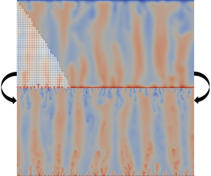
Figure 4. Snapshots of instantaneous mass concentration fields at $Ra=20\,000$ and $Sc=1$ . (a) DNS with $H/s=50$ and $\unicode[STIX]{x1D719}=0.56$ ( $s/d=1.5$ ). Here, the macroscopic mass concentration was obtained by volume averaging the microscopic mass concentration over each REV; (b) DNS with $H/s=20$ and $\unicode[STIX]{x1D719}=0.56$ ( $s/d=1.5$ ); (c) DOB simulation.

The instantaneous species concentration fields obtained from our DNS and DOB simulations at $Ra=20\,000$ are shown in figure 4. The macroscopic species concentration field $\langle c\rangle$ was either obtained from the DNS results by volume averaging over each REV (figure 4 a,b), or calculated directly in DOB simulations (figure 4 c). Both DNS and DOB mass concentration fields exhibit two boundary layer regions and an interior region. The interior region is dominated by transient mega-plumes, whereas the boundary layers are filled with small proto-plumes. These small proto-plumes are products of the growing instabilities in the boundary layers that cause low concentration fluid to rise and high concentration fluid to sink.

Interestingly, the instantaneous species concentration fields obtained by DNS and displayed in figures 4(a) and 4(b) suggest that the size of mega- and proto-plumes increases with the pore size. This phenomenon is absent in classical Rayleigh–Bénard convection (without a porous medium) and cannot be captured by the DOB equations where pore effects enter the equations only via $Ra$ .

Figure 5. Instantaneous profiles (a) and average spectra (b) of the dimensionless mass concentration, ${\hat{c}}$ , at mid-height $x_{2}/H=0.5$ . $Ra=20\,000$ , $\unicode[STIX]{x1D719}=0.56$ ( $s/d=1.5$ ) and $Sc=1$ .

Figure 5 shows several instantaneous profiles of ${\hat{c}}$ along with their corresponding time-averaged discrete Fourier transforms at mid-height for $Ra=20\,000$ and $Sc=1$ . The mean concentration $\langle {\hat{c}}\rangle ^{x1}$ , where the operator $\langle \cdot \rangle ^{x1}$ denotes horizontal averaging, was extracted from  ${\hat{c}}$ . The number of ${\hat{c}}$ maxima, which corresponds to the number of mega-plumes, decreases with increases in pore size $s$ (see figure 5 a). In the DOB simulations, the peak amplitude occurs when the wavenumber $k$ equals $9\unicode[STIX]{x03C0}$ . Wen et al. (Reference Wen, Corson and Chini2015) indicted that the wavenumber is not unique for $Ra>39\,716$ . However, the wavenumber is well approximated by $k=0.48Ra^{0.4}$ when $Ra$ is smaller than this critical value. Figure 6 shows that our DOB results are close to this correlation, as well as to the DOB results of Hewitt et al. (Reference Hewitt, Neufeld and Lister2012) and Wen et al. (Reference Wen, Corson and Chini2015). A variability of the peak wavenumber due to long-time-scale fluctuations was observed in Hewitt et al. (Reference Hewitt, Neufeld and Lister2012) when different initial field or aspect ratio ( $L/H$ ) were used, see hollow circles in figure 6. This variability was not found in our study since the same initial field and aspect ratio were used in both our DNS and DOB solutions.

In the DNS, the peaks are broader and the dominant wavenumber increases from $4\unicode[STIX]{x03C0}$ to $7\unicode[STIX]{x03C0}$ as $H/s$ increases from 20 to 50. This emphasizes the importance of the pore scale $s$ in shaping the mega-plumes. Motions at even larger length scales ( $k\approx \unicode[STIX]{x03C0}$ ), which corresponds to the length of the box ( $2H$ ), were observed in the DNS.

Figure 6. Peak wavenumber $k$ for the mega-plumes of the DOB results for different Rayleigh numbers. The maximum error bar for the peak wavenumber is estimated according to the wavenumber step size $\unicode[STIX]{x0394}k=\unicode[STIX]{x03C0}$ in our discrete fast Fourier transform (FFT).

Figure 7 shows several instantaneous profiles of ${\hat{c}}$ and their corresponding time-averaged Fourier transforms for $Ra=20\,000$ and $Sc=250$ . Similar to the results for $Sc=1$ , the dominant wavenumber increases from $4\unicode[STIX]{x03C0}$ to $7\unicode[STIX]{x03C0}$ as $H/s$ increases from 20 to 100. Here, the smallest Darcy number $Da$ is $3.5\times 10^{-7}$ , which corresponds to $H/s=100$ . Large-length-scale ( $k=\unicode[STIX]{x03C0}$ ) motions were also found in this test case, which makes the DNS results distinctly different from the DOB results. However, more detailed investigations are required to clarify the origin of these motions. We expect that the plumes will keep getting smaller as $H/s\rightarrow \infty$ and may even eventually converge toward the DOB results, see figure 8. However, although $Re_{k}$ for the DNS case is much smaller than 1 (see figure 3 b for $H/s=50$ ) and the pore size $s$ ( $0.01H$ for $H/s=100$ ) is much smaller than the plume size (approximately $0.23H$ for $Ra=20\,000$ , the DOB results), the peak wavenumbers from the DNS results are still clearly different from the DOB results. A possible reason is that no matter how small the pore size, the pore-scale structure may always affect part of the boundary layer in the vicinity of the wall.

Figure 7. Instantaneous profiles (a) and average spectra (b) of the dimensionless mass concentration, ${\hat{c}}$ , at mid-height $x_{2}/H=0.5$ , $Ra=20\,000$ , $\unicode[STIX]{x1D719}=0.56$ ( $s/d=1.5$ ) and $Sc=250$ .

Figure 8. Peak wavenumber $k$ for the mega-plumes of the DNS results for different Darcy numbers, $Ra=20\,000$ . The maximum error bar for the peak wavenumber is estimated according to the wavenumber step size $\unicode[STIX]{x0394}k=\unicode[STIX]{x03C0}$ in our discrete FFT.

4.2 Sherwood number

The scaling of the Sherwood number for $Sc=1$ obtained from our DNS results, with various $H/s$ and porosity values, is shown in figure 9. The DOB simulations of Hewitt et al. (Reference Hewitt, Neufeld and Lister2012) and our own DOB results are compared with our DNS results (shown by solid and dashed lines in figure 9 a). It appears that the DOB simulations overestimate the mass transfer rate for $Ra$ in the range between 600 and 4000, whereas at large $Ra$ , they fall amidst the values obtained by DNS for the porosities studied here. Although the scale ratio $H/s$ appears to determine the scale of mega-plumes, it only mildly influences $Sh$ and without a clear trend.

Figure 9. Time- and surface-averaged Sherwood number. Lines, DOB results; symbols, DNS results. The porosity $\unicode[STIX]{x1D719}$ and scale ratio $H/s$ are varied. The results for $Sc=1$ are shown in a log–log scale (a), and a linear scale for $Ra>5000$  (b).

The DNS results show that the porosity has a significant effect on $Sh$ in the high Rayleigh number regime ( $Ra>10\,000$ ). For example, at $Ra=20\,000$ , $Sc=1$ and $H/s=20$ , $Sh$ decreases from 158 to 96 while the porosity increases from $\unicode[STIX]{x1D719}=0.36$ ( $s/d=1.25$ ) to 0.56 ( $s/d=1.5$ ). At large Rayleigh numbers ( $Ra>5000$ ), the relationship between $Sh$ and $Ra$ can be well approximated by $Sh=8+0.0076Ra$ for $\unicode[STIX]{x1D719}=0.36$ . This linear relationship is in accordance with our own DOB results (Kränzien & Jin Reference Kränzien and Jin2019), as well as the DOB results by Hewitt et al. (Reference Hewitt, Neufeld and Lister2012). However, for $\unicode[STIX]{x1D719}=0.56$ , the correlation $Sh=0.033Ra^{0.8}$ better fits the data.

The Sherwood number slightly increases as the Schmidt number is increased from 1 to 250. However, the relationship between $Sh$ and $Ra$ does not change qualitatively (see figure 10). At large Rayleigh numbers ( $Ra>5000$ ), the Sherwood number is still higher for a lower porosity. The $Sh=f(Ra)$ scaling changes from a linear scaling ( $Sh=16+0.0076Ra$ ) for $\unicode[STIX]{x1D719}=0.36$ to a nonlinear one ( $Sh=0.045Ra^{0.8}$ ) for $\unicode[STIX]{x1D719}=0.56$ . The exponential coefficients for $Sc=250$ are the same as those for $Sc=1$ ( $\unicode[STIX]{x1D6FC}=1$ for $\unicode[STIX]{x1D719}=0.36$ and $\unicode[STIX]{x1D6FC}=0.8$ for $\unicode[STIX]{x1D719}=0.56$ ), which indicates that the relationship between $Sh$ and $Ra$ does not change qualitatively if $Sc$ is varied. Our DNS results suggest that the nonlinear scaling laws found in the experiments by Backhaus et al. (Reference Backhaus, Turitsyn and Ecke2011) and Neufeld et al. (Reference Neufeld, Hesse, Riaz, Hallworth, Techelepi and Huppert2010) may be related to the porosity or pore-scale factors, such as the pore size  $s$ .

Figure 10. The time and surface (over the wall surface) averaged Sherwood number, $Sc=250$ . Lines, DOB results; symbols, DNS results. The porosity $\unicode[STIX]{x1D719}$ and scale ratio $H/s$ are varied. The results are shown in the log scale (a) and linear scale for $Ra>5000$  (b).

It is worth noting that the small Schmidt number ( $Sc=1$ ) cases could also be representative of convective heat transfer in a porous medium with a Prandtl number of $Pr=1$ , which is common. However, in an experiment for heat transfer, Keene & Goldstein (Reference Keene and Goldstein2015) found a significantly smaller scaling exponent for the Nusselt number, $Nu\sim Ra^{0.319}$ . The possible cause of this discrepancy is that conjugate heat transfer may play an important role, as we here assumed that the wall surfaces of the porous elements are adiabatic because we considered mass transfer. Clearly, the effect of conjugate heat transfer on convection in porous media deserves further investigation.

4.3 Mass concentration and velocity statistics

Figure 11 shows the vertical profiles of the temporally and horizontally averaged macroscopic mass concentration $\langle \overline{{\hat{c}}}\rangle ^{x1}$ obtained from DOB simulations. Here, the species concentration profiles at different $Ra$ numbers become almost identical when the distance from the lower wall $\hat{x}_{2}$ is normalized by $1/Ra$ . This is in accordance with the statement by Huppert & Neufeld (Reference Huppert and Neufeld2014) that the boundary layer thickness is determined by $1/Ra$ . More details of our DOB results can be found in Kränzien & Jin (Reference Kränzien and Jin2019).

Figure 11. DOB results. (a) vertical profiles of time- and line-averaged species concentration; (b) root mean square (r.m.s.) of species concentration fluctuation $\langle {\hat{c}}^{rms}\rangle ^{x1}$ ; (c)  $u_{1}$ fluctuation; (d)  $u_{2}$ fluctuation.

By contrast, the profiles computed by resolving the flow at the pore scale with DNS exhibit a distinct length scale. Figure 12 shows strong deviations from the DNS results if $\hat{x}_{2}$ is scaled with $1/Ra$ . However, similar trends are observed if $\hat{x}_{2}$ is scaled with the pore scale ${\hat{s}}=s/H$ (figure 13). To explain this, one need to recall that the pore size $s$ can be approximated by using  $s^{\ast }$ , defined in (3.3) for a general two-dimensional porous matrix. The influence of the bounding walls is generally limited to within the first three REVs next to the walls, which leads to a steep gradient of $\langle \overline{{\hat{c}}}\rangle ^{x1}$ therein. When the distance from the lower wall is normalized by the pore size  $s$ , the $\langle \overline{{\hat{c}}}\rangle ^{x1}$ obtained at different Rayleigh numbers collapse together. Hence, the boundary layer thickness for convection in porous media is not determined by $Ra$ , but by the pore size  $s$ .

Figure 12. Vertical profiles of time- and line-averaged mass concentration for $Sc=1$ , DNS results. ▫: $H/s=20$ , $\unicode[STIX]{x1D719}=0.36$ , $Ra=5000$ . ○: $H/s=20$ , $\unicode[STIX]{x1D719}=0.56$ , $Ra=5000$ . +:  $H/s=20$ , $\unicode[STIX]{x1D719}=0.56$ , $Ra=20\,000$ . ×:  $H/s=50$ , $\unicode[STIX]{x1D719}=0.56$ , $Ra=5000$ .

Figure 13. DNS results for $Sc=1$ . (a) Vertical profiles of time- and line-averaged mass concentration; (b) r.m.s. of mass concentration fluctuation; (c)  $u_{1}$ fluctuation; (d)  $u_{2}$ fluctuation. ▫: $H/s=20$ , $\unicode[STIX]{x1D719}=0.36,Ra=5000$ . ○: $H/s=20$ , $\unicode[STIX]{x1D719}=0.56$ , $Ra=5000$ . +:  $H/s=20$ , $\unicode[STIX]{x1D719}=0.56$ , $Ra=20\,000$ . ×:  $H/s=50$ , $\unicode[STIX]{x1D719}=0.56$ , $Ra=5000$ .

Figure 13 also shows the r.m.s. macroscopic mass concentration and velocity fluctuations, $\langle {\hat{c}}^{rms}\rangle ^{x1}$ , $\langle \hat{u} _{1}^{rms}\rangle ^{x1}$ , and $\langle \hat{u} _{2}^{rms}\rangle ^{x1}$ , respectively, for $Sc=1$ . The velocity fluctuations were normalized with the characteristic velocity, $u_{m}=\unicode[STIX]{x1D6FD}\unicode[STIX]{x0394}cgK/\unicode[STIX]{x1D708}$ . The DNS results show that, besides $Ra$ , the scale ratios $H/s$ and porosity $\unicode[STIX]{x1D719}$ also have significant effects on r.m.s. quantities. These effects are absent in DOB simulations. In addition, $\langle \hat{u} _{1}^{rms}\rangle ^{x1}$ in figure 13(c) is distinctly different from the DOB results, which have unphysical (non-zero) velocity fluctuations at the wall surface (Hewitt et al. Reference Hewitt, Neufeld and Lister2012; Kränzien & Jin Reference Kränzien and Jin2019). A possible reason for these discrepancies is that momentum dispersion is not accounted for in the DOB equations.

Figure 14. DNS results for $Sc=250$ . (a) Vertical profiles of time- and line-averaged mass concentration; (b) r.m.s. of mass concentration fluctuation; (c)  $u_{1}$ fluctuation; (d)  $u_{2}$ fluctuation. ▫: $H/s=20$ , $\unicode[STIX]{x1D719}=0.36$ , $Ra=5000$ . ○: $H/s=20$ , $\unicode[STIX]{x1D719}=0.56$ , $Ra=5000$ . +:  $H/s=20$ , $\unicode[STIX]{x1D719}=0.56$ , $Ra=20\,000$ . ×:  $H/s=50$ , $\unicode[STIX]{x1D719}=0.56$ , $Ra=20\,000$ .

Figure 14 shows the temporally and horizontally averaged macroscopic results for $Sc=250$ . Similar to the results for $Sc=1$ (see figure 13), the influence of the bounding walls is still limited to within the first three REVs next to the walls. Again, our DNS results confirm that the boundary layer thickness for convection in porous media is determined by the pore size $s$ (or $s^{\ast }$ for a porous matrix with permeability $K$ and porosity  $\unicode[STIX]{x1D719}$ ).

As the boundary layer thickness is determined by the pore size (which can be characterized by the square root of the permeability, $\sqrt{K}$ ), the momentum dispersion term $\unicode[STIX]{x2202}(\unicode[STIX]{x1D719}\langle \text{}^{i}{\tilde{u} _{i}\,}^{i}\tilde{u} _{j}\rangle ^{i})/\unicode[STIX]{x2202}\hat{x}_{j}$ and the viscous diffusion term $(Sc/\unicode[STIX]{x1D6FE}_{m}Ra)(\unicode[STIX]{x2202}^{2}\hat{u} _{i}/\unicode[STIX]{x2202}\hat{x}_{j}^{2})$ in the macroscopic equation (2.9) are expected to scale as $1/K$ . Thus, the momentum dispersion and viscous diffusion terms should be of order $1/Da=H^{2}/K$ , exactly as the Darcy term itself. Thus, our DNS results suggest that the pore scale significantly influences convection in porous media through the momentum dispersion and viscous diffusion terms, which are neglected in the DOB equations. We conclude that these terms cannot be neglected in the macroscopic equations even if the pore size is small. In addition, the pore size should be used as the characteristic length when the dispersion term is modelled.