Comparison of Alternative Pulpwood Inventory Strategies and Machine Systems at a Log-Yard Using Simulations


1
Department of Forest Biomaterials and Technology, Swedish University of Agricultural Sciences, SE-901 83 Umeå, Sweden
2
Swedish Cluster of Forest Technology, Kuratorvägen 2A, SE-907 36 Umeå, Sweden
*
Author to whom correspondence should be addressed.
Forests 2020, 11(4), 373; https://doi.org/10.3390/f11040373
Submission received: 12 February 2020
/
Revised: 13 March 2020
/
Accepted: 17 March 2020
/
Published: 26 March 2020
(This article belongs to the Special Issue Supply Chain Optimization for Biomass and Biofuels)
Abstract
:The rising throughput of log-yards imposes new constraints on existing equipment and increases the complexity of delivering an optimal and uninterrupted supply of pulpwood to pulp mills. To find ways of addressing these problems by reducing log cycle times, this work uses a discrete-event mathematics model to simulate operations at a log-yard and study the impact of three different log-yard inventory strategies and two alternative machine systems for log transportation between main log-yard and buffer storage. The yard’s existing inventory strategy of last load in and first out limits access to older logs at the main storage site. By allocating space for 89,000 m3 and 99,000 m3 of pulpwood at the buffer storage it is possible to keep the log cycle time at the main storage to a maximum of 12 and 6 months. Additionally, the use of an alternative log transportation machine system comprising a material handler with a trailer increased the work time capacity utilization relative to the yard’s current machine system of two shuttle trucks and a material handler for transporting logs between the main and buffer storage areas. Compared to the currently-used last in first out inventory strategy and purposely emptying the main storage area once or twice per year did reduce the total work time of both machine systems by 14% and 30%. Consequently, the volume delivered from the buffer to the log-yard decreased on average by 17% and 37% when emptying the main storage area once and twice per year. Even with reduced work time when emptying the main storage area, both machine systems could fulfil given work load for transporting logs from the buffer storage to the main log-yard without interrupting operations of the log-yard.
1. Introduction
Sweden is a large pulp producer, accounting for 8.8% of the world’s total pulp production in 2016 [1]. Over the last 16 years, the number of operational pulp mills in Sweden has decreased from 45 to 40, while the average production capacity per mill has increased by 27%, reaching 320,000 t pulp per mill [2]. These developments present significant challenges for supply chain logistics because of the need to ensure uninterrupted production at the mills while maintaining a competitive price for the delivered pulpwood as the supply area increases. Introducing intermediate terminals between the forest and the mill is one way to cope with the increased supply area and uncertainty in inventory keeping at the mill’s log-yard [3,4,5]. However, extra material handling steps at terminals increase the overall cost of the delivered wood [5,6]. An alternative way of maintaining a pulpwood inventory level capable of supporting mill operations is to have a large log-yard at the mill’s gate that can accommodate the incoming pulpwood volume.
In comparison to sawmills, pulp mills usually handle only one roundwood assortment - pulpwood. Major concerns in pulpwood log handling are log freshness and the logs’ physical location in the yard [7]. Because there is no need to separate different roundwood assortments at a pulp mill’s log-yard, there is a risk that storage areas operated under the first in-last out (FILO) storage principle may become too large. In such cases, the logs that are delivered first may be locked-in at the bottom of stacks, where they gradually lose freshness and quality, potentially to the point that they become unsuitable for pulping [8,9]. Over a prolonged period of time, this causes financial loses for a pulp mill. Breaking up such large storage areas into smaller ones can reduce log cycle times in the yard and thereby avoid this problem. However, the physical area available for log storage at the yard is often limited. Consequently, the only way to maintain a yard’s storage capacity while increasing the fragmentation of its inventory is often to increase the height of stockpiles or to establish a buffer storage area close to or within the yard. The scope for expanding a log-yard at a mill may be limited by various constraints; notably, it may restrict the use of existing machines without additional investments in log-yard infrastructure. On the other hand, introducing new machines at a log-yard also requires significant investment. All these options thus involve significant financial and operational risks to the uninterrupted operation of the pulp mill, making a careful risk analysis essential [10].
Given the diverse constraints on log-yards, it can be difficult to find ways of making changes that improve efficiency. For instance, introducing a new machine to overcome infrastructure constraints so as to avoid construction work requires consideration of machine and construction costs as well as machine work patterns and how they will integrate with the yard’s existing machine park. Optimization by trial and error in such cases is very risky because it could introduce inefficiencies if done without a good understanding of machine interactions, space utilization, product cycle times, equipment work cycle times, and the decision-making logic of machine operators, all of which profoundly influence pulpwood throughput at log-yards.
A rational way of supporting decision-making is to use mathematical modelling [11,12]. The core benefit of mathematical modelling is that it allows systems to be analysed in a way that reveals the parameters and logic governing a given situation. A software representation of a mathematical model is known as a computer simulator, and performing simulations is a fast and cheaper way to evaluate different plans before implementing them in practice.
Authors including Asikainen [13], Karttunen et al. [14], Arriagada et al. [15], Eriksson [16], Pinho et al. [17], Chiorescu and Gronlund [18] and Salichon [19] have used simulations to investigate, design and optimise operational processes in the forest industry ranging from timber harvesting to wood supply and processing. In addition, Mendoza et al. [20], Beaudoin et al. [21], Rahman et al. [22] used simulations to optimize log in-feed and log sorting at sawmills’ log-yards, and to characterize yard operations. While modelling and simulations have been used for a few decades in forestry, relatively few modelling studies have focused on log-yards and specifically on pulpwood log-yards.
Several methods can be used to mathematically analyse forest operations and log-yards [23,24,25]. One whose variations have been commonly used in forestry is discrete-event modelling (DEM) and discrete-event simulation (DES), which is well suited for analysing log-yard systems because the processes at log-yards follow a sequence of discrete events similar to the production lines of other industrial processes [26,27]. In the DEM framework, we can mathematically describe physical attributes of incoming wood and processes it has to pass through by defining under what conditions each process can be initiated and how much time it takes to complete it before the wood can proceed to the next stage in the system.
The company studied in this article operates a log-yard for a pulp mill. The log-yard receives logs via three modes of transportation: trucks, trains and ships. Unloading these logs can necessitate challenging decision-making during daily operations because the space in the main log-yard is limited and the company wants to maintain a high inventory level to minimize the risk of running out of raw material. Arriving logs are placed in three main storage areas which follow the last in first out (LIFO) queuing principle. Because of the continuous arrival of new logs, it is difficult to avoid the lock-in effect in the biggest storage area. The yard therefore uses a nearby buffer storage area when its main storage capacity is exhausted and to reduce the incidence of lock-in at the main yard. The yard’s infrastructure does not allow the existing log-stackers to leave the main log-yard area, so an external machine park is used to move logs from the buffer area to the main yard. The company’s interest is to explore alternative inventory keeping strategies and find out whether it would be possible to improve their operations by introducing a new type of machine to move logs between the buffer area and the main yard. Therefore the first objective was to evaluate if a new machine system can fulfil the work load requirements of moving logs between buffer area and main log-yard area. The existing and new machine system’s performance was evaluated under three different inventory management strategies at the main log-yard. The second objective was to analyse the effect of the three inventory management strategies on the main yard’s log cycle time and their effect on the storage capacity required in the buffer area.
2. Materials and Methods
The analysis presented here is based on data supplied by the company that owns the studied log-yard, Domsjö Fiber AB. These data include detailed information about when trucks, trains and ships arrived at the yard and the volume of logs they carried. Additionally, short time studies were conducted to observe the log-stackers’ work cycles and thereby better understand their productivity and work logic. Comparatively little data were available on other aspects of the yard’s operations because access was limited and some contractors were unwilling to be observed while working at the yard. Therefore, information on the log-yard’s storage capacity and storage areas, the decision-making process at the yard, and the pulp mill’s daily volume requirements were obtained via interviews with log-yard and logistics managers. The base model and the analysis of company data on which this study is based were described by Kons et al. [12]. The company’s yearly data were divided into 52 data sets of which half were used for analysis and model building. The model’s parameters were set per week because the company has a weekly pulpwood demand. The simulated results represent the yard’s operations over a year, and the simulations are focused on the dynamics of the log inventory levels at the yard.
The yard receives log deliveries via three modes of transport (trucks, trains, and ships), each of which has a different carrying capacity. Because the delivery volumes of each mode differ greatly, they were normalized against the volume supplied by a single truck [12]. That is to say, the delivery volumes of trains and ships were expressed in terms of the carrying capacity of a truck; each train and ship delivery was represented as 36 and 132 trucks arriving simultaneously, respectively. Normalization was necessary to enable realistic analysis of the work of log stackers and other machines at the yard, and to allow for work interruptions when working on volumes delivered by train or by ship; unloading a train or ship takes several hours, whereas a single truck can be unloaded in minutes [12].
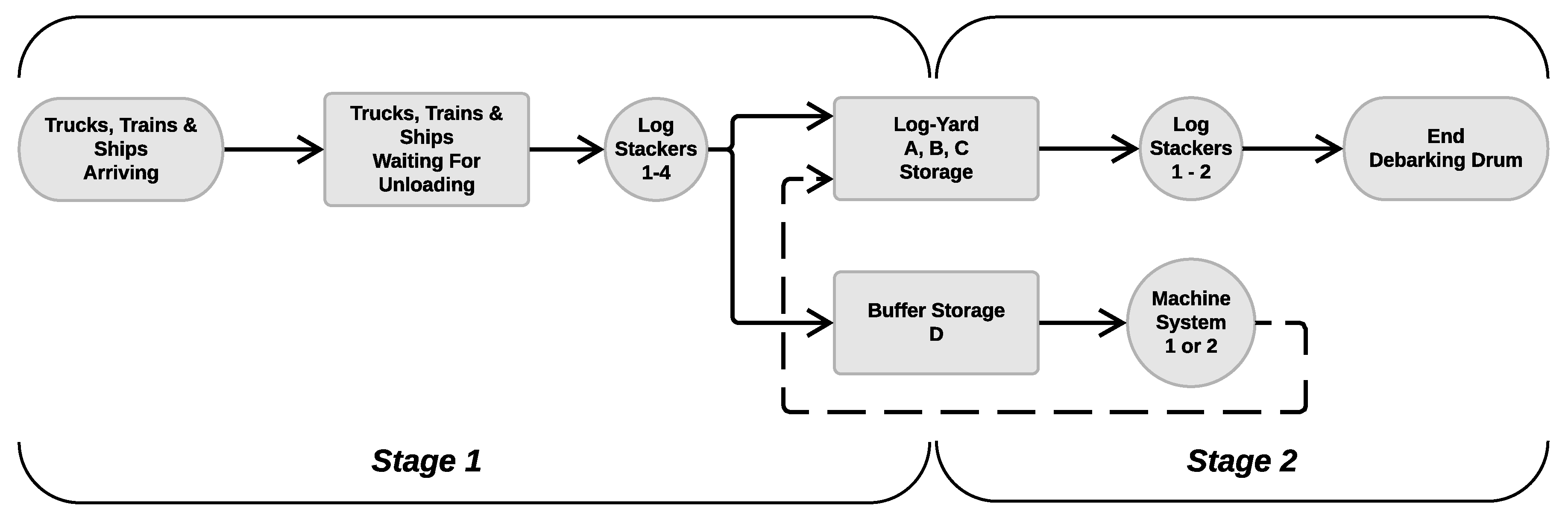
2.1. Stage 1
The processing of logs can be divided into two stages (Figure 1). Stage 1 covers the unloading of logs delivered to the yard by truck, train, and ship. Deliveries may arrive on five days of the week. The company’s data indicate that approximately one ship and one train arrive each week. Since there was insufficient data to generate a probability density function (PDF) to model train and ship arrival, the inter-arrival interval (dt) for all modes of transport was based on the truck data and was modelled using a generalized Pareto probability density function (1) as described by Kons et al. [12]. The company’s pulpwood demand rose to 22,600 m3/week in 2018; it was assumed that this would leave the shape of the dt PDF unchanged but shorten the dt interval. The PDF has the form:
where is the input value, is the shape parameter (0.3080), is the scale parameter (0.00320) and is the threshold parameter (0.00361). These values were derived by least squares regression.
The company’s data indicate that the probabilities of arrival of trucks, trains, and ships are 99.2%, 0.3% and 0.5%. The model was configured such that if a train or ship arrived during a given week, no further arrivals by the same mode of transport could occur during that week. The quantity dt is based on the yard’s working hours and the fact that it is open for five days per week, including nights. Transport units generated during weekends are therefore removed before entering the waiting queue for unloading.
After the volume of one truck load (ca. 38.9 m3) was determined using a weighted PDF based on a normal distribution (with a mean of 45.4302 m3 and a standard deviation of 4.5819 m3) and a uniform distribution (with lower and upper bounds of 1 m3 and 30 m3, respectively), the total normalized delivery volumes by different modes of transport was determined against those for trucks. The weights of the normal and uniform components were 0.78 and 0.22, respectively [12]. Weighted PDFs were needed to account for split truckloads, in which only part of the load is delivered to the pulp mill; such deliveries accounted for 22% of the volume supplied to the mill (2).
where and are the weights 22% and 78% according to data, and , are the normal and uniform PDFs defined as (2b) and (2c), where and are the input values, is the mean value (45.4302), is standard deviation (4.5819), is the lower end point (minimum 1), is the upper endpoint (maximum 30).
Once the transport unit arrives, it enters a waiting queue for unloading by one of the four log-stackers operating at the log-yard. The number of working log-stackers is decided based on the queue lengths of the waiting transport units. If the waiting transport queue is less than three units, only one log-stacker will be active. If the queue is between three and five units, an extra log-stacker is called out. If the queue becomes five to seven units, the third log-stacker is called out. If the transport queue becomes longer than seven transport units, all four log-stackers work simultaneously.
The time taken to unload logs is described by a normally distributed PDF with a mean of 319 s and a standard deviation of 75 s.
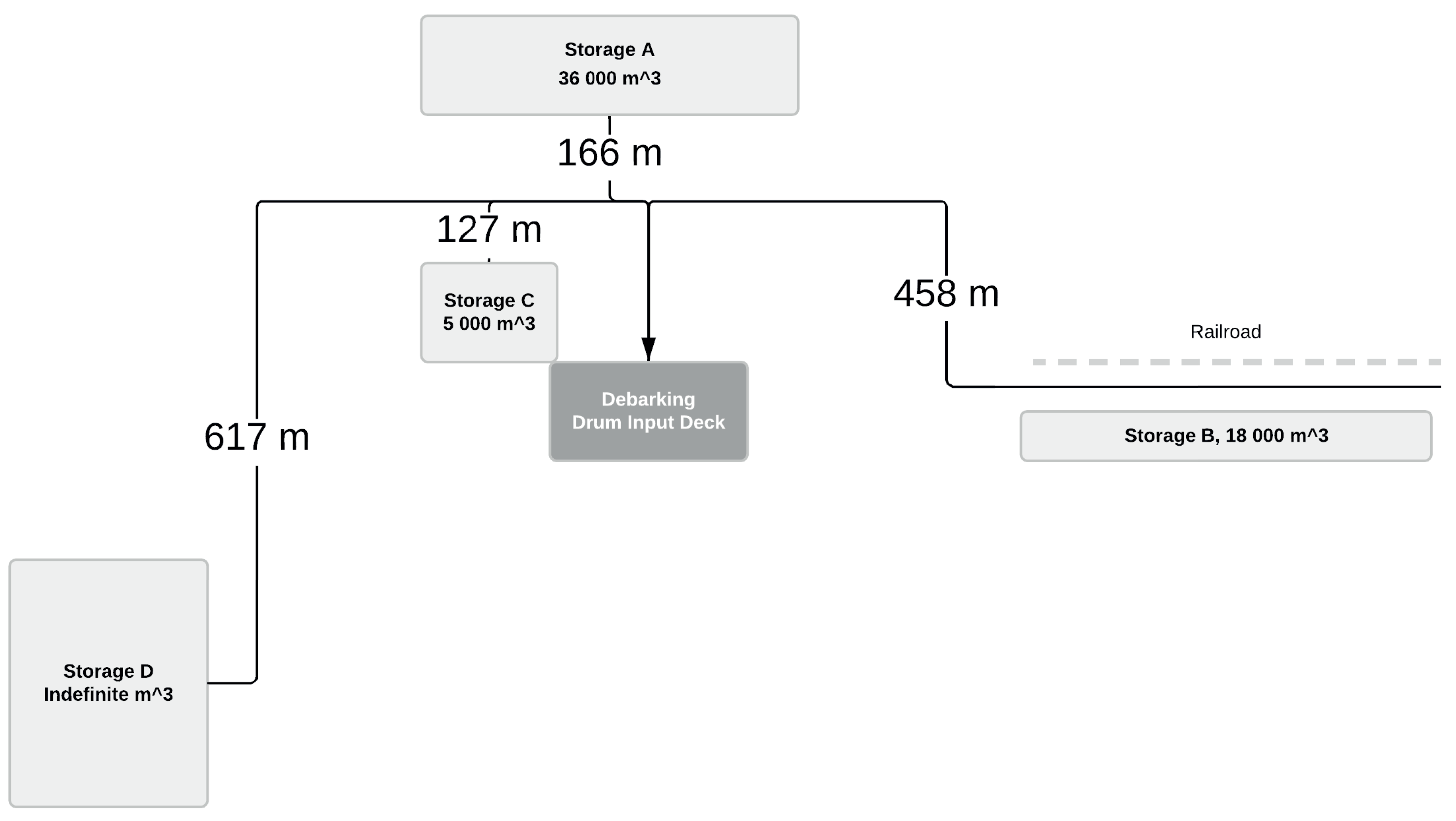
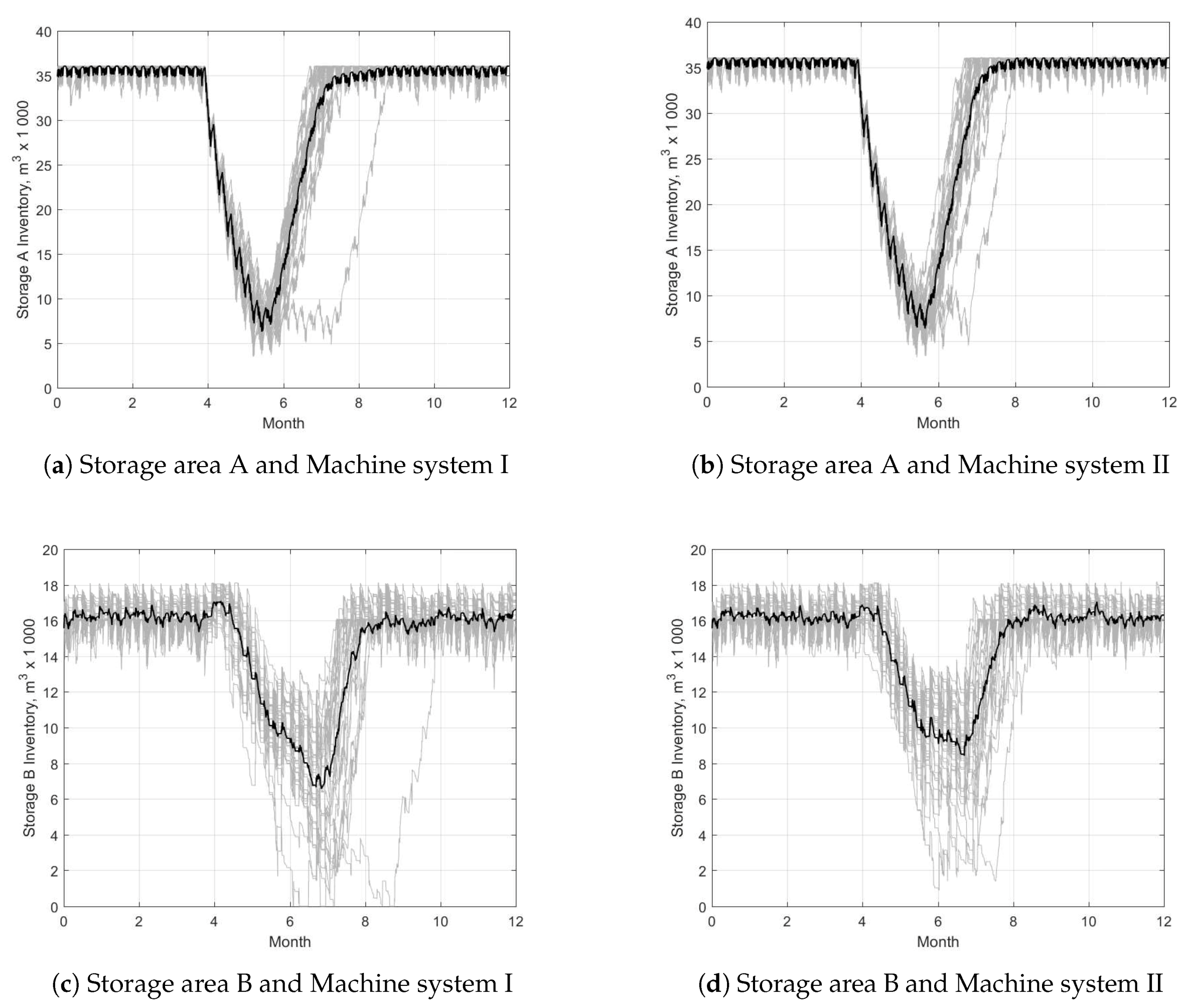
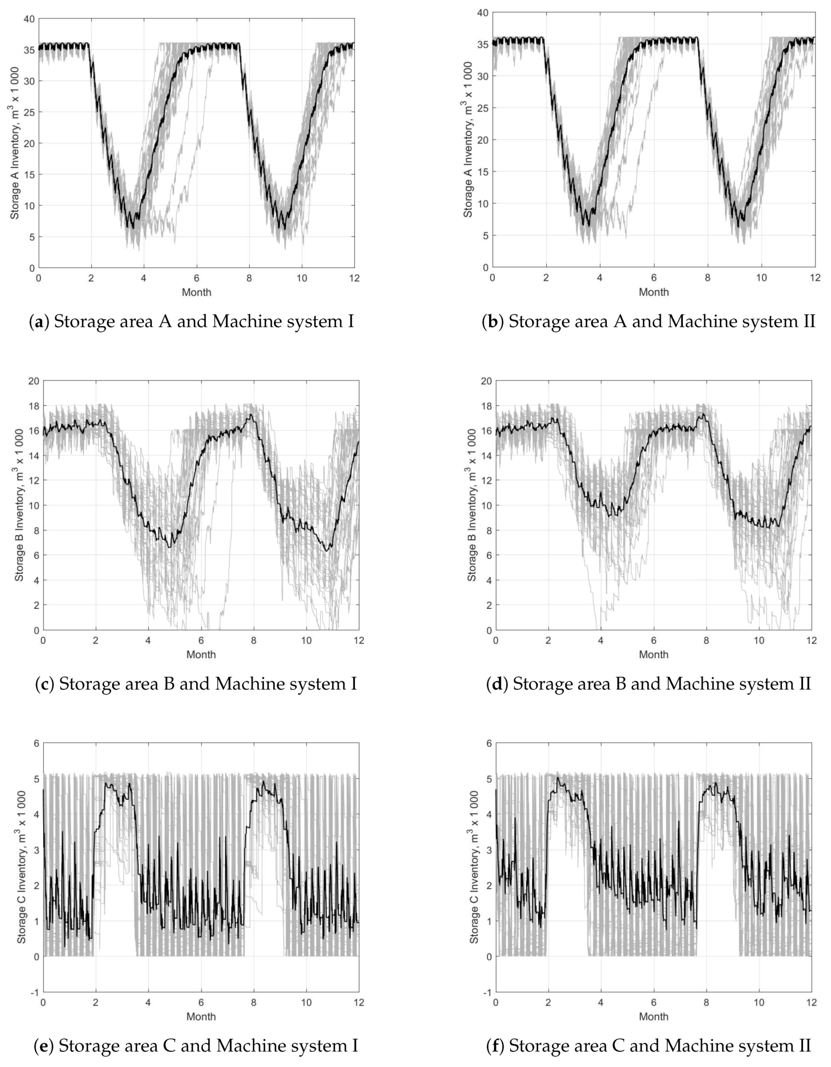
The log-yard has four distinct storage areas (A, B, C, and D) whose maximum storage capacities are, respectively, 36,000 m3, 18,000 m3, 5000 m3, and unlimited. Of these four storage areas A, B and C is considered as main log-yard while area D is buffer storage which is scattered around in a bigger close by area within the pulp mill territory. All four storage areas operate on the LIFO principle, meaning that the last log load to arrive is the first to leave the storage area.
Volume delivered by truck is placed in storage area A, while deliveries by train and ship are placed in storage areas B and C, respectively (Figure 2). Area D provides buffer storage capacity that is used when areas A, B, or C are full. If storage area A is full when a truck delivery arrives but the inventory level at area B is below 16,000 m3, the logs in the delivery will be unloaded at area B. However, if the inventory level at area B is above 16,000 m3, the logs will be unloaded at the buffer storage area (D). Logs that would normally be placed in storage areas B or C are redirected to area D if the inventory levels at those areas are above 18,000 m3 and 5000 m3, respectively. Stage 1 ends when the logs are unloaded in one of the four storage areas.
2.2. Stage 2
In stage 2, according to [28] to ensure that log-yard is not empty the four storage areas are pre-loaded at the start of the simulation in such a way that the total volume of logs stored at the yard is at least 70,000–75,000 m3, in accordance with the company’s minimum objectives. Storage areas A, B, C and D are pre-loaded with 900, 400, 120, and 400 normalized truck units, respectively, corresponding to stored volumes of approximately 35,000 m3, 15,500 m3, 4660 m3 and 15,500 m3, respectively.
The log stackers used in Stage 1 are also used in Stage 2 to move logs from the main log-yard to the debarking drum. Each log stacker’s work time is restricted to 18h per day for four days and 12 h for one day. During weekends, the log-stackers do not work at all. Given these constraints, the time taken for a log stacker to move one unit of logs at a rate compatible with the pulp mill’s weekly pulpwood demand of 22,600 m3 can be described using a normal PDF with a mean of 513 s and standard deviation of 154 s.
Because of infrastructural constraints, log stackers can only work in storage areas A, B, and C. This gives rise to two questions relating to the management of inventory levels in the four storage areas and the machine systems used to move logs from buffer storage area D back to the main log-yard. For supply security reasons log-yard managers want to ensure that the total inventory level at all four storage areas does not fall much below 70,000 m3. Therefore, areas A, B and C must be filled to capacity at all times. However, managers also want the stored logs to be reasonably fresh. Unfortunately, the storage of logs in piles forces the yard to operate according to the LIFO principle, which creates a “lock-in” effect whereby the logs that arrive at the yard first are “trapped” at the bottom of the log stacks. To minimize the adverse impact of lock-in on pulpwood quality, the logs can be redistributed to the buffer storage area (D) periodically, allowing the main storage areas to be emptied. This reduces the overall log cycle time.
2.3. Inventory Strategies
Storage area A is the biggest and the most important part of the log-yard. Because of its high number of incoming trucks and the fact that the yard operates on the LIFO principle, there is a particularly high risk that logs will be locked-in for long periods of time in this area. To address this problem, three different log-yard inventory strategies are compared in order to determine the effect of periodically emptying storage area A on buffer storage and machine system transporting logs back to the log-yard. The log-yard’s managers have little long term control over what is delivered or when it arrives, so the main way they can control inventory levels in the log-yard is by deciding how much volume should be removed and brought to the pulp mill from each storage area.
Strategy I is the “Business As Usual” case, which represents the yard’s current approach (Table 1). In this case, the log stackers visit each storage area at a frequency that keeps the inventory levels at each area in relative balance and minimizes the need to take logs to the buffer area. The relative frequencies at which log stackers visit areas A, B, and C are 57%, 8%, and 35%, respectively. However, this working pattern creates a high risk of lock-in at the biggest storage area (A) because the continuous arrival of new logs limits access to the older logs in the log stack at the back of the storage.
Under Strategy II, lock-in at storage area A is alleviated by emptying area A once per year. During this process, the logs arriving for storage A are temporarily redirected to the buffer storage area (D). While this process is ongoing, 5% of the incoming volume that would normally be delivered to area A is directly redirected to area D in order to reduce the time needed to empty area A. Under this strategy, the relative frequency at which log stackers visit storage area A is overwritten from day 116 onwards if the inventory level at area A is above 5000 m3. This is maintained until the inventory level in area A falls to 5000 m3, which represents less than one day’s demand from the pulp mill. At this point, it is assumed that all of the remaining logs in area A can be removed while new log stacks are built and so the storage area is emptied. Therefore, when the inventory level in storage area A reaches 5000 m3, the relative frequency at which log stackers visit area A is restored to the value used in Strategy I, and logs from the buffer area can be returned to the main yard.
Strategy III assumes that log freshness is even more valuable and therefore calls for storage area A to be emptied twice per year. In this case, the relative frequency at which log stackers visit area A is overwritten (in the same way as in Strategy I) from day 58 onwards if the inventory level at area A is above 5000 m3. The stacker visit frequency is then reset to the Strategy I value once the inventory level at area A has fallen to 5000 m3. During this period, 5% of the volume incoming to area A is immediately redirected to storage area D. This process of emptying storage area A before returning to Strategy I is repeated after an additional 232 days.
Under all three inventory management strategies, logs stored in the buffer area must be returned to the log-yard and fed into the debarking drum. At present, the log-yard’s infrastructure restricts the log stackers’ access to the buffer area, so an external contractor must be hired to transport logs from the buffer to the main log-yard. This arrangement is referred to as Machine System I (Table 1). To obtain more flexibility in the planning and control of log flow within the log-yard, its managers are considering buying an alternative machine setup (Machine System II). The performance and constraints of these machine systems were compared under each of the three inventory management strategies outlined above.
Machine System I consists of a material handler and two shuttle trucks with trailers, and is used to move logs from buffer storage D to storage area C in the log-yard. All three machines under Machine System I are operated by the contractor, who must be called when needed and can only operate when the conditions permit at least one full shift (8 h) of continuous work. Machine System I has an average productivity of 156 m3/h; in the model, the variation in its productivity is described using a normal PDF for the time taken to serve one normalized truck load unit according to Functions (2a)–(2c); the mean and standard deviation of this PDF are 900 s and 270 s, respectively. When logs are brought back from buffer storage D, they are placed in storage area C, which is otherwise used to store logs delivered by ship and is the storage area closest to the debarking drum’s in-feed. Therefore, for the contractor to be called out, the inventory level in storage area C must be 500 m3 or less (to ensure there is sufficient space) and must not exceed 2300 m3 to leave storage space for incoming ship deliveries. At the same time, the inventory level in buffer storage D must be at least 1300 m3 to ensure there is sufficient volume for a full working shift. The contractors can work for at most 8 h per day, five days a week.
Machine System II consists of a self-loading material handler with a trailer that works for the same 84 h per week as the log stackers at the log-yard. Machine System II is only used to transport logs from the buffer area to storage area C in the log-yard. The average productivity of Machine System II is 62 m3/h, and the variability of the time taken to move one unit with this machine system was modelled using a normal distribution with a mean of 2250 s and a standard deviation of 675 s. We assume that the log-yard owns the machine and can operate it daily with less strict inventory level conditions in storage areas C and D. Therefore, there is no lower limit on the inventory level in buffer storage D when using Machine System II because it is not necessary to provide sufficient work for a full working shift. Additionally, because Machine system II can work continuously every day, the inventory level required at storage area C to initiate transportation from buffer area D is set to 3000 m3. When the inventory level at storage area C reaches 4000 m3, log transportation is stopped.
Under all three inventory management strategies, the transport units and the corresponding log volumes exit the system upon delivery to the debarking drum by a log stacker.
2.4. Analysis and Statistics
All data analyses, modeling, and simulations were performed using MathWorks’ MATLAB and the Simulink software packages.
In total, six scenarios were analysed representing every possible combination of inventory management strategy and machine system. The log inventory dynamics under the three strategies were then compared. Additionally, the effect of machine systems I and II on inventory dynamics was investigated along with differences in the machine systems’ working patterns. Each scenario was simulated 30 times, giving a total of 180 simulation runs. After each run, data for each storage area and the total inventory levels over time were recorded. Additionally, data from the block representing the two different machine systems were recorded to evaluate machine work time and the volume of transported logs. Finally, the total volume generated and delivered to the debarking drum was recorded. According to Banks et al. [29], to verify that the model accurately represents the log-yard’s operations, we compared its inputs and outputs to those reported by the company managers and to the company’s data. Additionally, the machine work time and volume carried were verified to be within the maximum permitted working hours and below the machines’ capacity, respectively. The statistical significance of differences between scenarios was tested using the Mann-Whitney two-tailed T-test (P < 0.05) and One-way ANOVA, and the Kruskal-Wallis test with Dunn’s correction (P< 0.05).
3. Results
The differences between scenarios with respect to the average volume of pulpwood arriving at the yard were insignificant (0.51%). The differences between scenarios in terms of the average volume delivered to the pulp mill were slightly larger but still insignificant (0.75%; see Table 2).
The log-yard’s average total inventory level varied by no more than 5248 m3 (Table 3) under any scenario. Additionally, the incoming and delivered volumes were very similar under all scenarios; the average difference between the total incoming and delivered volume was 1967 m3 (Table 2).
However, the scenarios did differ significantly (P < 0.05) with respect to the distribution of the total volume between storage areas A, B, C, and D. The average yearly volumes at areas A and B under strategy II were 13% and 9% lower, respectively, than under strategy I, while those under strategy III were 15% and 13% lower, respectively, than under strategy II. Conversely, the average yearly volumes at areas C and D under strategy II were 28% and 13% higher, respectively, than under strategy I, while those under strategy III were 21% and 8% higher, respectively, than under strategy II.
Varying the machine system used to transport logs between areas C and D had no significant effect on the inventory strategies (Table 3). However, there were differences in the machines’ work patterns. On average, the total working time of Machine System II was 189% greater than that of Machine System I due the lower overall productivity per hour and more flexible working conditions of the Machine System II (Table 4). Additionally, the total working times of both machine systems under strategy II were 14% lower than under strategy I, with a further 16% decrease between strategies II and III. Despite the large differences in total work time between machine systems I and II, the volumes they transported differed less markedly. On average, Machine System II transported 16% more volume per year than Machine System I. In keeping with the work time results, the delivered volume under strategy II was 17% lower than under strategy I, and that for strategy III was 20% lower than under strategy II (Table 4).
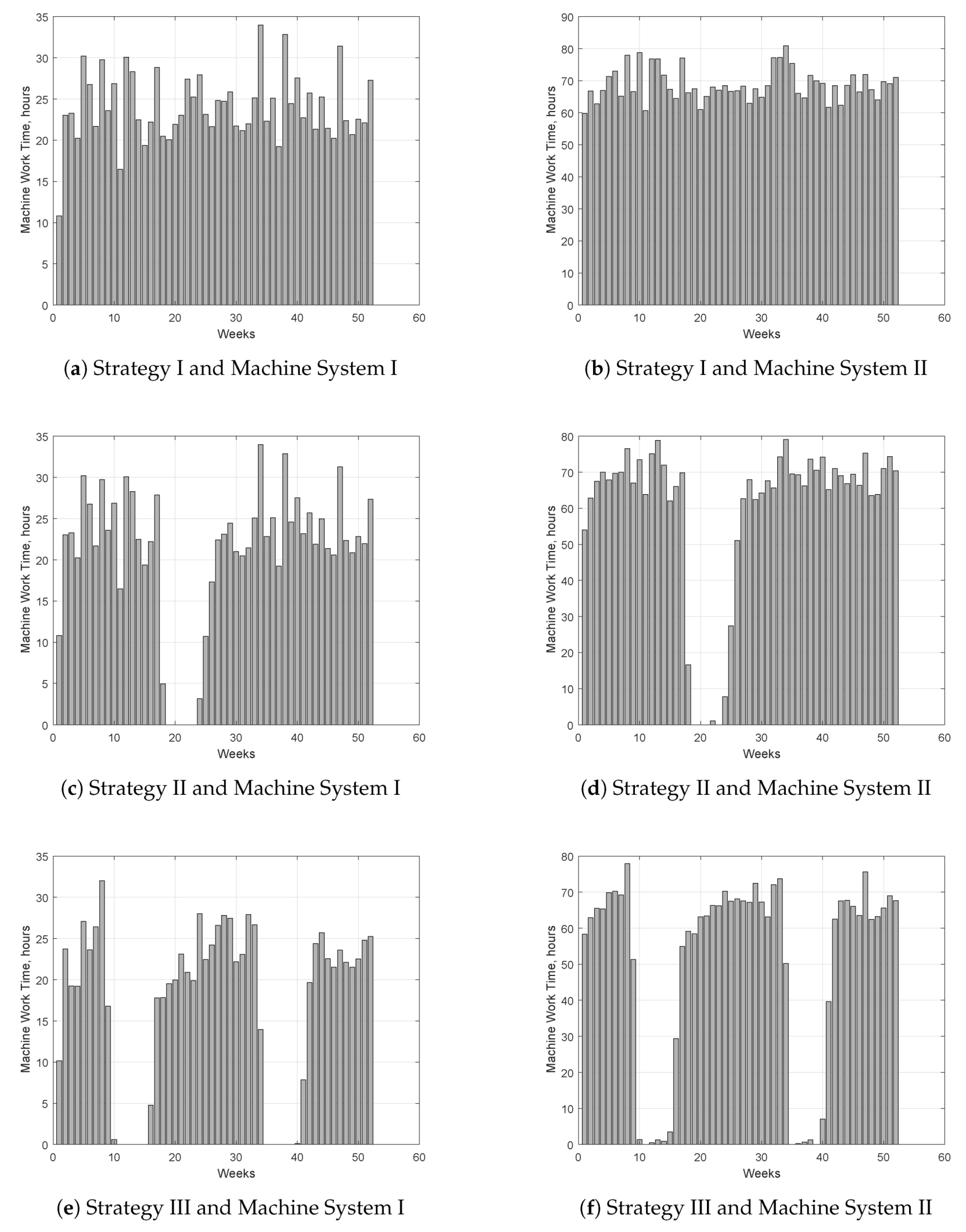
Over the year, the work time distribution of Machine System II was slightly smoother and more evenly distributed from week to week than that of Machine System I (Figure 3). Moreover, Machine System II could still be used during periods when storage area A was being emptied and storage area C was close to its maximum capacity for receiving logs from the buffer storage.
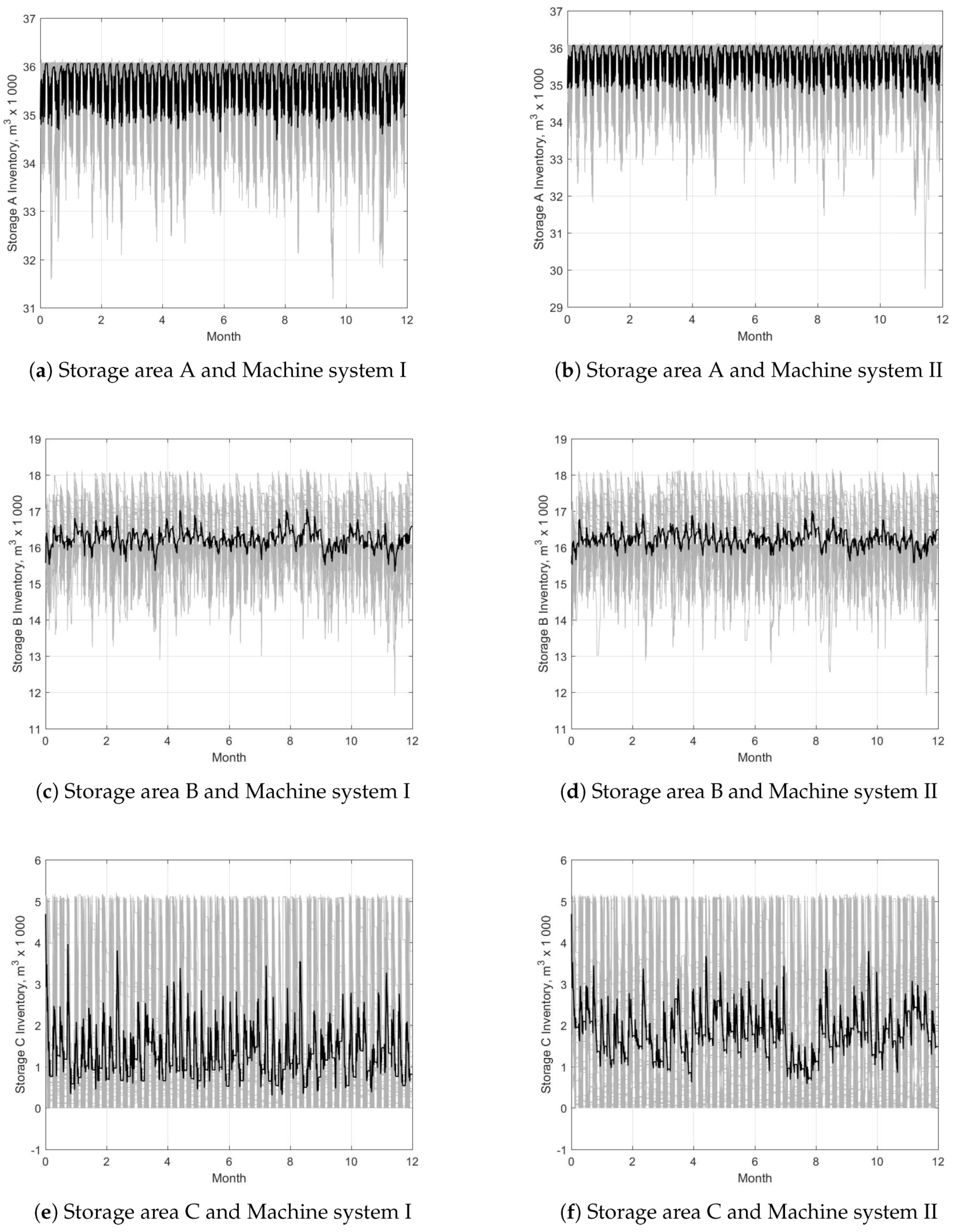
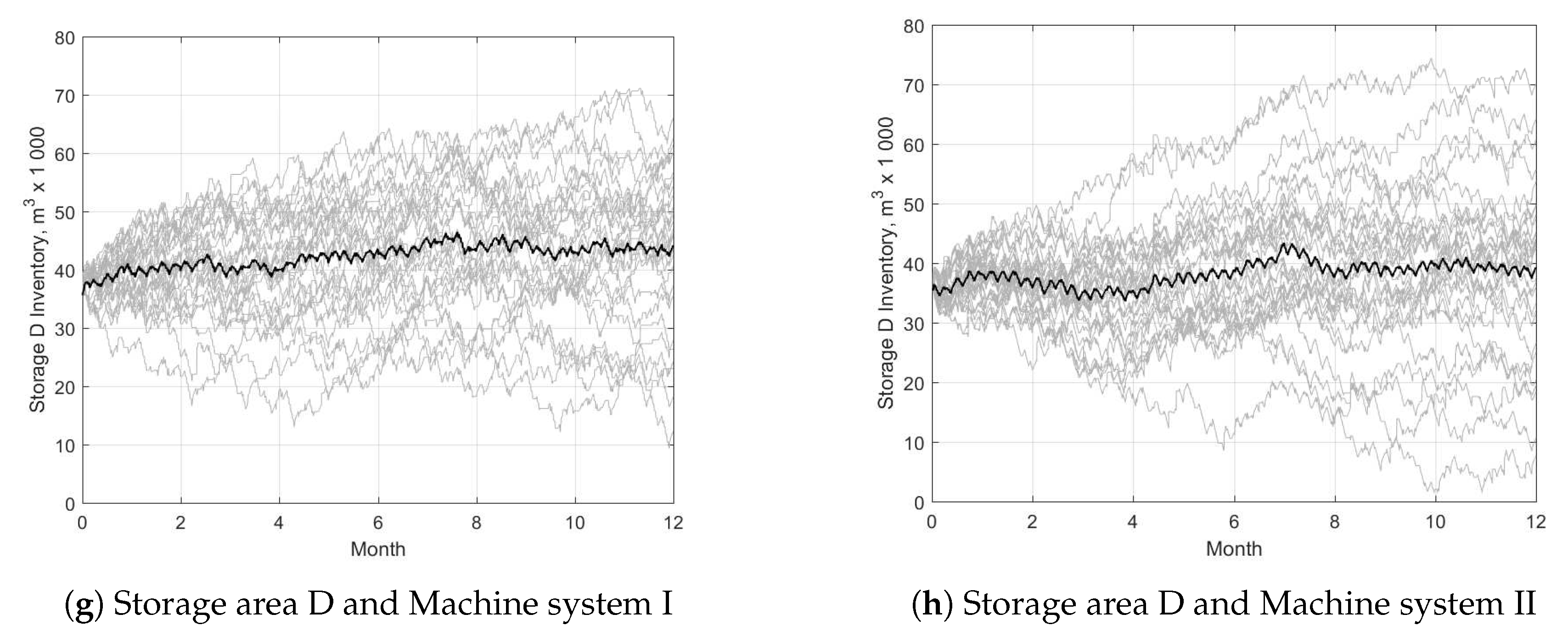
Figure 4 shows the yearly inventory changes over one year under Strategy I for Machine Systems I and II. The average inventory level is very close to the average maximum and average minimum values because the volume flows in all four storage areas were relatively consistent over the year. Even when looking at the absolute maximum and minimum values under both machine systems over 30 simulations, the inventory level variation at storage areas A and B was relatively small (ca. 6000 and 6300 m3, respectively), and both areas remained close to their maximum capacities (Figure 4). The variation in maximum and minimum inventory levels in storage areas C and D was much more pronounced. Storage area C could go from empty to full (ca. 5000 m3) in a matter of days when a ship was unloaded. Additionally, because the purpose of area D is to accommodate changing volume flows, its average stored volume varied by as much as 67,000 m3.
In Strategy II, storage area A is emptied once per year, which reduces the average inventory levels of storage areas A and B while increasing those of areas C and D (Figure 5). In scenarios S2 M1 and S2 M2, the time of the year during which the storage A reaches its minimum inventory level varied by as much as 63 and 47 days, respectively, depending on the inflow of material. While storage area A was being emptied, machine work due to haulage of logs between areas D and C stopped for two full weeks under scenario S2 M1 and for four weeks under scenario S2 M2. Once the inventory level in storage A reached its minimum value, the machine work and storage levels returned to almost their initial values.
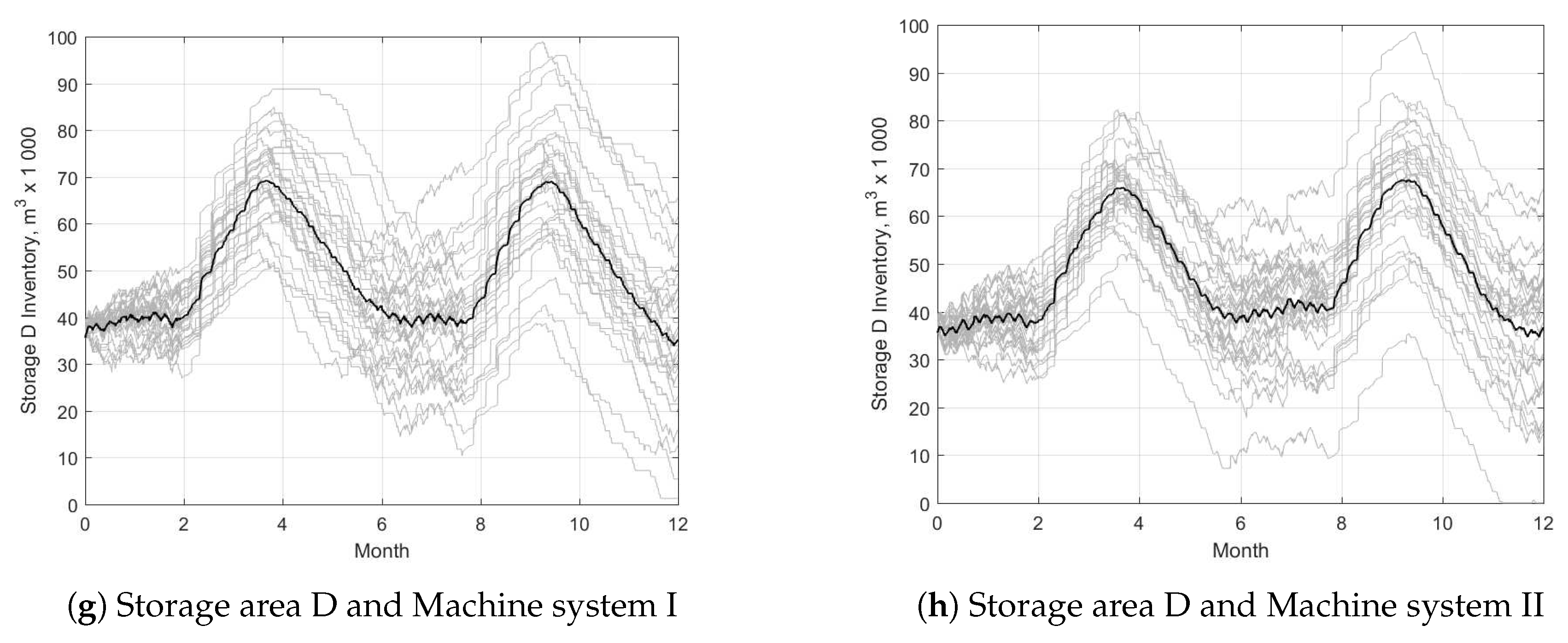
Under strategy III, storage area A is emptied twice yearly, and lock-in is avoided by reducing the log turnover time to around six months (Figure 6). With both machine systems, under Strategy III, the volume held at storage area A reaches its first minimum after 55 days of emptying; reaching the second minimum takes 31 for Machine System I and 21 days for Machine System II. Because storage area A is emptied twice per year, the average inventory levels of the storage areas change even more markedly than under Strategy II. Additionally, while storage area A is being emptied, machine work due to transportation of logs between storage areas D and C is halted for 10 full weeks when using Machine System I, and 3 weeks for Machine System II.
The main driver of log-yard storage dynamics are the incoming and outgoing volumes. While the arriving and delivered volumes to the mill do not vary greatly (Table 2), they have an effects on the fluctuations in buffer storage as even a slight increase of incoming traffic can trigger even more prerequisite condition to redirect excess volumes to the buffer storage. As result this effects also the time required to empty area A (Figure 4, Figure 5 and Figure 6). This modest variation in combination with inventory strategy and machine use causes substantial variation in the total inventory level, which ranged from 40,832 to 130,262 m3 under different scenarios.
4. Discussion
Lock-in effects of the logs were avoided at all four storage areas (A, B, C and D) when the total minimum inventory level of the whole log-yard was held below 60,000 m3, as was the case for strategies II and III. However, while the log-yard did not run out of logs in any of the simulation runs, maintain such low inventory levels would substantially increase the risk of pulpwood shortages. Under Strategy I, maintaining an absolute minimum inventory level of less than 10,000 m3 also creates the possibility of avoiding lock-in in storage areas C and D, assuming that there is space to use a stack layout that provides access to logs in storage area D (Figure 4). However, given the pulp mill’s weekly pulpwood demand of ca. 22,600 m3, reducing the yard’s inventory level to less than 60,000 m3 creates a major risk of raw material insecurity for the pulp mill. When the log-yard’s inventory is so low, an additional supply of pulp chips to the pulp chip buffer storage should be secured to compensate for the lack of pulpwood logs. Additional pulp chip storage helps to even out the demand for the pulpwood supply and makes logistics planning easier. However, pulp chip storage is a short term storage in order to keep the pulp chip quality acceptable and it is not included in the study.
The results for the average wood flows revealed that only storage area C exhibited no lock-in under any strategy. Under Strategy I, to maintain the yard’s total inventory at the desired level of 75,000–125,000 m3, all three of the yard’s main storage areas are held close to their maximum capacity at all times. Under strategies II and III, lock-in is disrupted at storage areas A and C at least once or twice per year (Figure 5 and Figure 6a,b,e,f). This is achieved by redirecting some of the incoming volume to storage area D, which works as a buffer storage. In storage areas B and D, the configuration of the storage area plays a significant role in preventing lock-in (or at least minimizing its occurrence). Storage area B is a long area with two log stacks facing one-another. As shown in Figure 5 and Figure 6, this area reaches its minimum average inventory level of ca. 7000–9000 m3 (which is around half its capacity) once or twice per year. With well-planned machine work, these drops in inventory levels could enable the removal of older logs from this area, thereby avoiding lock-in. One way to plan work in this way would be to manually track each end of the elongated log stacks and empty them from one end at a time. This would require data on log arrival times and placement, which could be used to develop a suitable algorithm using approaches established in studies on the industrial packaging problem [30]. Area D is the yard’s biggest storage area. In this work, it is assumed to have an unlimited capacity and a large area. When storage area A is managed according to Strategy I, the average inventory level of storage area D stabilizes at ca. 40,000 m3 (Table 3). The lowest average volume delivered from area D to area C is 135,830 m3/year (Table 4). Under these circumstances, with a well-planned log stack configuration, the log storage period should be no longer than one year, even at area D.
To make log-yard operations and inventory levels smooth, it is important to have sufficient machine capacity for transporting logs from storage area D to C. Table 3 shows that inventory levels at storage areas C and D are almost independent of the machine system under all three strategies, although Machine System II causes the inventory level at area D to be slightly lower and that at area C to be slightly higher than is observed with Machine System I. This difference relates directly to the composition of the two machine systems. Machine system I is like a hot system in that each of its units is highly dependent on the others. Consequently, careful planning and well-defined conditions are needed to utilize it optimally. Conversely, Machine System II is like a cold system in that a single machine unit can load/unload and transport smaller volumes at its own pace at almost any time because it has much less strict operational requirements. Additionally, Machine System II was assumed to have the same weekly working hours as the other log-yard machines (84 h/week). The two machine systems thus have different operational environments. As a result, Machine System II delivers more volume back to the log-yard than Machine System I and has more working hours per year (Table 4) and (Figure 3).
Both machine systems were assumed to deliver logs from storage area D to storage area C. However, Machine System I is operated by a contractor who is only called in when needed, whereas Machine System II is assumed to belong to the log-yard. Therefore the working hours of Machine System II could be increased further because the log-yard owners could use it in other more remote parts of the yard when storage area C is too full to take logs from area D.
It is very challenging to model an existing log-yard with enough accuracy to reproduce real-world decision-making and performance outcomes. When using DEM-based models, such accuracy requires large amounts of data representing a long period of time. Unfortunately, this is rarely possible because such data are rarely collected by companies, log-yard workers may be unwilling to be recorded, and safety considerations may prevent observation of certain areas of the yard. The results presented here relied on data representing one year of the studied yard’s operations. However, it is impossible to guarantee that a single year of data will be fully representative of the yard’s operations over a multi-year period. Additionally, like Robichaud et al. [31], we relied heavily on short time studies and interviews with log-yard managers when modelling the decision-making processes that govern the yard’s operations and also when analysing performance-related data. The problem with short term time studies and decision-making data provided by log yard managers is that they do not necessarily reflect real yard operations over extended periods; instead, they may simply reflect the operational environment that managers would like to see. The lack of long-term data is particularly problematic when modelling decision-making relating to log flows within the log-yard because it necessitates the inclusion of many conditional statements and outcomes often deviates from norms over longer time periods.
To further improve the yard’s performance and reduce log turnaround times in each storage area, algorithms and potentially even new log-yard layouts could be developed using concepts from packing problem theories [32]. Since the log-yard handles large bulk volumes, even small improvements in log accessibility and storage times could confer noticeable financial and operational benefits [30].
In conclusion, the results presented here show that when the maximum storage capacity at storage area D reaches around 89,000 m3, which is a ca. 16,000 m3 increase relative to that used at present, and it opens up a possibility to empty storage area A once per year, even when the inflow of material to the log-yard is at its highest (Figure 5). Storing an additional 10,000 m3 (total 99,000 m3) at area D makes it possible to empty storage area A twice per year, halving the log turnaround time at (Figure 6). Additionally, the yard’s existing machine systems for transporting logs from area D to area C are fully capable of handling the volumes of material necessary to keep the log-yard running while implementing these strategies. These results can be used to provide the initial decision support for the yard’s managers, enabling them to avoid the lock-in of logs at the yard and to evaluate alternative machine systems for log handling.
Author Contributions
Conceptualization, K.K., P.L.H. and D.B.; methodology, P.L.H. and K.K.; software, K.K. and P.L.H.; validation, K.K. and P.L.H.; formal analysis, K.K.; investigation, K.K.; resources, D.B. and P.L.H.; data curation, K.K. and P.L.H.; writing–original draft preparation, K.K., P.L.H. and D.B.; writing—review and editing, K.K., P.L.H. and D.B.; visualization, K.K. and P.L.H.; supervision, D.B. and P.L.H.; project administration, D.B.; funding acquisition, D.B. All authors have read and agreed to the published version of the manuscript.
Funding
This research was part of the BioHub project financed by the Botnia-Atlantica program, under the European Regional Development Fund.
Acknowledgments
The authors gratefully acknowledge the help of Domsjö Fiber AB for providing data regarding log-yard operations.
Conflicts of Interest
The authors declare no conflict of interest and the funders had no role in the design of the study; in the collection, analyses, or interpretation of data; in the writing of the manuscript, or in the decision to publish the results.
References
- FAO. Pulp and paper capacities. In Survey 2016–2021, Forest Policy and Rescources Division; FAO Forestry Department: Rome, Italy, 2017. [Google Scholar]
- Swedish Forest Industries Federation. Produktion Och Handel Med Massa 2018 [Production and Trade of Pulp 2018]; Statistik Om Skog Och Industri: Stockholm, Sweden, 2019. [Google Scholar]
- Enström, J.; Athanassiadis, D.; Öhman, M.; Grönlund, O. Satsa Pårätt Bränsleterminal [Aim for the Right Biomass Terminal]; Report; Skogforsk: Uppsala, Sweden, 2013. [Google Scholar]
- Kons, K.; Bergström, D.; Eriksson, U.; Athanassiadis, D.; Nordfjell, T. Characteristics of Swedish forest biomass terminals for energy. Int. J. For. Eng. 2014, 25, 238–246. [Google Scholar] [CrossRef]
- Virkkunen, M.; Kari, M.; Hankalin, V.; Nummelin, J. Solid Biomass Fuel Terminal Concepts and a Cost Analysis of a Satellite Terminal Concept; VTT Technology 211; Technical Research Centre of Finland (VTT): Espoo, Finland, 2015. [Google Scholar] [CrossRef]
- Väätäinen, K.; Prinz, R.; Malinen, J.; Laitila, J.; Sikanen, L. Alternative operation models for using a feed-in terminal as a part of the forest chip supply system for a CHP plant. Gcb Bioenergy 2017, 9, 1657–1673. [Google Scholar] [CrossRef] [Green Version]
- Liukkoxs, K.; Elowsson, T. The effect of bark condition, delivery time and climate-adapted wet storage on the moisture content of Picea abies (L.) Karst. pulpwood. Scand. J. For. Res. 1999, 14, 156–163. [Google Scholar] [CrossRef]
- Nahmias, S. Perishable inventory theory: A review. Oper. Res. 1982, 30, 680–708. [Google Scholar] [CrossRef] [PubMed]
- Persson, E. Storage of Spruce Pulpwood Effects on Wood and Mechanical Pulp. Ph.D. Thesis, Department of Forest Management and Products, Swedish University of Agricultural Sciences, Uppsala, Sweden, 2001. [Google Scholar]
- March, J.G.; Shapira, Z. Managerial perspectives on risk and risk taking. Manag. Sci. 1987, 33, 1404–1418. [Google Scholar] [CrossRef] [Green Version]
- Robinson, S. Simulation: The Practice of Model Development and Use; John Willey and Sons: Chichester, UK, 2004; Volume 1, p. 5. [Google Scholar]
- Kons, K.; La Hera, P.; Bergström, D. Modelling Dynamics of a Log-Yard Through Discrete-Event Mathematics. Forests 2020, 11, 155. [Google Scholar] [CrossRef] [Green Version]
- Asikainen, A. Simulation of stump crushing and truck transport of chips. Scand. J. For. Res. 2010, 25, 245–250. [Google Scholar] [CrossRef]
- Karttunen, K.; Lättilä, L.; Korpinen, O.J.; Ranta, T. Cost-efficiency of intermodal container supply chain for forest chips. Silva Fenn. 2013, 47, 24. [Google Scholar] [CrossRef] [Green Version]
- Arriagada, R.A.; Cubbage, F.W.; Abt, K.L.; Huggett, R.J., Jr. Estimating harvest costs for fuel treatments in the West. For. Prod. J. 2008, 58, 24. [Google Scholar]
- Eriksson, A.; Eliasson, L.; Jirjis, R. Simulation-based evaluation of supply chains for stump fuel. Int. J. For. Eng. 2014, 1–14. [Google Scholar] [CrossRef]
- Pinho, T.M.; Coelho, J.P.; Moreira, A.P.; Boaventura-Cunha, J. Modelling a biomass supply chain through discrete-event simulation. IFAC-PapersOnLine 2016, 49, 84–89. [Google Scholar] [CrossRef]
- Chiorescu, S.; Gronlund, A. Assessing the role of the harvester within the forestry-wood chain. For. Prod. J. 2001, 51, 77. [Google Scholar]
- Salichon, M.C. Simulating Changing Diameter Distributions in a Softwood Sawmill. Master’s Thesis, Graduate School, Oregon State University, Corvallis, OR, USA, 2005. [Google Scholar]
- Mendoza, G.A.; Meimban, R.J.; Araman, P.A.; Luppold, W.G. Combined log inventory and process simulation models for the planning and control of sawmill operations. In Proceedings of the 23rd CIRP International Seminar on Manufacturing Systems, Nancy, France, 6–7 June 1991; p. 8. [Google Scholar]
- Beaudoin, D.; LeBel, L.; Soussi, M.A. Discrete Event Simulation to Improve Log Yard Operations. INFOR Inf. Syst. Oper. Res. 2013, 50, 175–185. [Google Scholar] [CrossRef] [Green Version]
- Rahman, A.; Yella, S.; Dougherty, M. Simulation model using meta heuristic algorithms for achieving optimal arrangement of storage bins in a sawmill yard. J. Intell. Learn. Syst. Appl. 2014, 6, 125–139. [Google Scholar] [CrossRef] [Green Version]
- Aalto, M.; Raghu, K.C.; Korpinen, O.J.; Karttunen, K.; Ranta, T. Modeling of biomass supply system by combining computational methods—A review article. Appl. Energy 2019, 243, 145–154. [Google Scholar] [CrossRef]
- Lättilä, L. Improving Transportation and Warehousing Efficiency with Simulation-Based Decision Support Systems. Ph.D. Thesis, Faculty of Technology Management, Industrial Management, Lappeenranta University of Technology, Lappeenranta, Finland, 2012. [Google Scholar]
- Taha, H.A. Operations Research: An Introduction, 5th ed.; Macmillan Publishing Company: New York, NY, USA, 1992; Volume 1. [Google Scholar]
- Kendall, K.; Mangin, C.; Ortiz, E. Discrete event simulation and cost analysis for manufacturing optimisation of an automotive LCM component. Compos. Part A Appl. Sci. Manuf. 1998, 29, 711–720. [Google Scholar] [CrossRef]
- Huka, M.A.; Gronalt, M. Log yard logistics. Silva Fenn. 2018, 52, 23. [Google Scholar] [CrossRef] [Green Version]
- Schroer, B.J.; Tseng, F.T. Modelling complex manufacturing systems using discrete event simulation. Comput. Ind. Eng. 1988, 14, 455–464. [Google Scholar] [CrossRef]
- Banks, J.; Carson, J.S., II; Nelson, B.L.; Nicol, D.M. Discrete-Event System Simulation; Pearson: London, UK, 2005. [Google Scholar]
- Hopper, E.; Turton, B. A genetic algorithm for a 2D industrial packing problem. Comput. Ind. Eng. 1999, 37, 375–378. [Google Scholar] [CrossRef]
- Robichaud, S.V.; Beaudoin, D.; Lebel, L. LOG YARD DESIGN USING DISCRETE-EVENT SIMULATION: FIRST STEP TOWARDS A FORMALIZED APPROACH. In Proceedings of the 10th International Conference of Modeling and Simulation-MOSIM’14, Nancy, France, 5–7 November 2014. [Google Scholar]
- Dowsland, K.A.; Dowsland, W.B. Packing problems. Eur. J. Oper. Res. 1992, 56, 2–14. [Google Scholar] [CrossRef]
Figure 1.
General layout of the logistics system at a pulp mill.

Figure 2.
Layout of log-yard’s storage areas with their storage capacities and distances to the input deck for debarking.
Figure 2.
Layout of log-yard’s storage areas with their storage capacities and distances to the input deck for debarking.

Figure 3.
Machine system I and II working hours per week under three different inventory keeping strategies when transporting logs from storage D to storage C.
Figure 3.
Machine system I and II working hours per week under three different inventory keeping strategies when transporting logs from storage D to storage C.

Figure 4.
Average of 30 yearly simulation results (black line) and individual results of 30 yearly simulations (grey lines) showing inventory level fluctuation at storage areas A, B, C, and D under Strategy I using Machine Systems I (left side) and II (right side) (S1 M1 and M2).
Figure 4.
Average of 30 yearly simulation results (black line) and individual results of 30 yearly simulations (grey lines) showing inventory level fluctuation at storage areas A, B, C, and D under Strategy I using Machine Systems I (left side) and II (right side) (S1 M1 and M2).


Figure 5.
Average of 30 yearly simulation results (black line) and individual results of 30 yearly simulations (grey lines) showing inventory level fluctuation at storage areas A, B, C, and D under Strategy II using Machine Systems I (left side) and II (right side) (S2 M1 and M2).
Figure 5.
Average of 30 yearly simulation results (black line) and individual results of 30 yearly simulations (grey lines) showing inventory level fluctuation at storage areas A, B, C, and D under Strategy II using Machine Systems I (left side) and II (right side) (S2 M1 and M2).


Figure 6.
Average of 30 yearly simulation results (black line) and individual results of 30 yearly simulations (grey lines) showing inventory level fluctuation at storage areas A, B, C, and D under Strategy III using Machine Systems I (left side) and II (right side) (S3 M1 and M2).
Figure 6.
Average of 30 yearly simulation results (black line) and individual results of 30 yearly simulations (grey lines) showing inventory level fluctuation at storage areas A, B, C, and D under Strategy III using Machine Systems I (left side) and II (right side) (S3 M1 and M2).


Table 1.
Tested combinations of machine systems and inventory management strategies for emptying storage area A.
Table 1.
Tested combinations of machine systems and inventory management strategies for emptying storage area A.
| Machine System | Empty Storage A | ||
|---|---|---|---|
| Strategy I a | Strategy II | Strategy III | |
| Machine System I a | At 57% rate | 1 time per year | 2 times per year |
| Machine System II | At 57% rate | 1 time per year | 2 times per year |
a reference system.
Table 2.
Yearly volume of pulpwood arriving at the log-yard and delivered to the pulp mill under different scenarios. and denote the strategy and machine system used in the scenario, respectively.
Table 2.
Yearly volume of pulpwood arriving at the log-yard and delivered to the pulp mill under different scenarios. and denote the strategy and machine system used in the scenario, respectively.
| Volume Arriving | Volume Delivered | |||
|---|---|---|---|---|
| Avg, m3 | STD, m3 | Avg, m3 | STD, m3 | |
| S1 M1 | 1,178,200 | 14,381 | 1,171,500 | 4397 |
| S1 M2 | 1,174,000 | 19,021 | 1,171,600 | 6745 |
| S2 M1 | 1,178,200 | 14,381 | 1,174,600 | 4402 |
| S2 M2 | 1,177,800 | 17,440 | 1,174,800 | 5064 |
| S3 M1 | 1,174,600 | 17,412 | 1,178,100 | 4170 |
| S3 M2 | 1,180,000 | 15,904 | 1,180,400 | 5659 |
Table 3.
Pulpwood inventory levels at the four storage areas and the total log-yard inventory level over the 52-week period under six scenarios based on 30 simulation results per scenario. The scenarios are given labels of the form Sx My where x is the number of the inventory strategy and y is the number of the machine system used to transport logs between storage areas D and C. The max and min values are the maximum and minimum volumes observed at the indicated storage area in any one of the 30 simulation runs for the indicated scenario. The Avg Max and Avg Min values (shown in parentheses) are the maximum and minimum values observed in the average of the 30 simulation runs for the indicated scenarios, and are plotted in black in Figure 4, Figure 5 and Figure 6.
| Scenario | Storage A | Storage B | Storage C | Storage D | Total Inventory | ||||||
|---|---|---|---|---|---|---|---|---|---|---|---|
| m3 | m3 | m3 | m3 | m3 | |||||||
| S1 M1 | Max (Avg Max) | 36,176 | (36,064) | 18,155 | (17,067) | 5203 | (4690) | 71,111 | (46,474) | 127,606 | (100,610) |
| Avg | 35,624 | 16,237 | 1317 | 42,220 | 95,422 | ||||||
| Min (Avg Min) | 31,181 | (34,467) | 11,898 | (15,329) | 0 | (305) | 9405 | (35,592) | 61,257 | (88,553) | |
| S1 M2 | Max (Avg Max) | 36,213 | (36,062) | 18,162 | (17,006) | 5200 | (4690) | 74,417 | (43,429) | 130,262 | (98,794) |
| Avg | 35,631 | 16,233 | 1825 | 38,104 | 91,828 | ||||||
| Min (Avg Min) | 29,489 | (34,527) | 11,898 | (15,515) | 0 | (578) | 1410 | (33,575) | 52,836 | (85,749) | |
| S2 M1 | Max (Avg Max) | 36,198 | (36,064) | 18,168 | (17,097) | 5203 | (5013) | 88,131 | (71,628) | 125,973 | (97,875) |
| Avg | 31,007 | 14,597 | 1776 | 46,166 | 93,569 | ||||||
| Min (Avg Min) | 3480 | (6275) | 0 | (6567) | 0 | (278) | 6275 | (35,592) | 58,163 | (85,553) | |
| S2 M2 | Max (Avg Max) | 36,217 | (36,068) | 18,206 | (17,060) | 5194 | (4912) | 89,196 | (70,178) | 124,874 | (98,351) |
| Avg | 31,093 | 14,893 | 2252 | 44,368 | 92,639 | ||||||
| Min (Avg Min) | 3218 | (6379) | 890 | (8424) | 0 | (756) | 2689 | (35,421) | 53,818 | (87,161) | |
| S3 M1 | Max (Avg Max) | 36,177 | (36,062) | 18,170 | (17,314) | 5191 | (4928) | 98,950 | (69,254) | 127,686 | (95,781) |
| Avg | 25,982 | 12,367 | 2209 | 49,594 | 90,174 | ||||||
| Min (Avg Min) | 2598 | (6008) | 0 | (6250) | 0 | (255) | 1260 | (33,932) | 40,832 | (83,995) | |
| S3 M2 | Max (Avg Max) | 36,269 | (36,062) | 18,148 | (17,362) | 5187 | (5032) | 98,511 | (67,599) | 126,683 | (98,816) |
| Avg | 26,552 | 13,320 | 2646 | 47,793 | 90,341 | ||||||
| Min (Avg Min) | 3438 | (6156) | 0 | (8078) | 0 | (731) | 0 | (34,678) | 43,630 | (84,851) | |
Table 4.
Yearly work time and volumes delivered from storage area D to storage area C by machine systems I and II over one year based on 30 simulation runs per scenario. The theoretical yearly full-time working hours for machine systems I and II are 2080 and 4368 h, respectively; the capacity utilization figures in the table are the ratios of their actual numbers of working hours in the simulations to these values.
| Productivity, m3/h | Work Time Per Year | Delivered Volume Per Year | ||||
|---|---|---|---|---|---|---|
| Avg, h | STD, h | Capacity Utilization, % | Avg, m3 | STD, m3 | ||
| S1 M1 | 156 | 1249 | 68 | 60.0 | 194,240 | 10,636 |
| S1 M2 | 62 | 3577 | 110 | 81.9 | 222,500 | 6892 |
| S2 M1 | 156 | 1068 | 81 | 51.3 | 166,020 | 12,517 |
| S2 M2 | 62 | 3065 | 113 | 70.2 | 190,450 | 7191 |
| S3 M1 | 155 | 875 | 83 | 42.1 | 135,830 | 12,938 |
| S3 M2 | 62 | 2579 | 156 | 59.0 | 160,340 | 9732 |
© 2020 by the authors. Licensee MDPI, Basel, Switzerland. This article is an open access article distributed under the terms and conditions of the Creative Commons Attribution (CC BY) license (http://creativecommons.org/licenses/by/4.0/).
Share and Cite
MDPI and ACS Style
Kons, K.; Hera, P.L.; Bergström, D. Comparison of Alternative Pulpwood Inventory Strategies and Machine Systems at a Log-Yard Using Simulations. Forests 2020, 11, 373. https://doi.org/10.3390/f11040373
AMA Style
Kons K, Hera PL, Bergström D. Comparison of Alternative Pulpwood Inventory Strategies and Machine Systems at a Log-Yard Using Simulations. Forests. 2020; 11(4):373. https://doi.org/10.3390/f11040373
Chicago/Turabian StyleKons, Kalvis, Pedro La Hera, and Dan Bergström. 2020. "Comparison of Alternative Pulpwood Inventory Strategies and Machine Systems at a Log-Yard Using Simulations" Forests 11, no. 4: 373. https://doi.org/10.3390/f11040373
Note that from the first issue of 2016, this journal uses article numbers instead of page numbers. See further details here.