A General Model for the Effect of Crop Management on Plant Disease Epidemics at Different Scales of Complexity


Department of Sustainable Crop Production, Facoltà di Scienze Agrarie, Alimentari e Ambientali, Università Cattolica del Sacro Cuore, via Emilia Parmense 84, 29122 Piacenza, Italy
*
Author to whom correspondence should be addressed.
†
Current Affiliation: Origin Enterprises plc, 4-6 Riverwalk, Citywest Business Campus, Dublin 24, Ireland.
Agronomy 2020, 10(4), 462; https://doi.org/10.3390/agronomy10040462
Submission received: 16 February 2020
/
Revised: 18 March 2020
/
Accepted: 24 March 2020
/
Published: 26 March 2020
(This article belongs to the Special Issue Plant Disease Epidemiology: Changing Perspectives, Emerging Technologies and Prediction Modeling)
Abstract
:A general and flexible model was developed to simulate progress over time of the epidemics caused by a generic polycyclic pathogen on aerial plant parts. The model includes all of the epidemiological parameters involved in the pathogen life cycle: between-season survival, production of primary inoculum, occurrence of primary infections, production and dispersal of secondary inoculum both inside and outside the crop, and concatenation of secondary infection cycles during the host’s growing season. The model was designed to include the effect of the main crop management actions that affect disease levels in the crop. Policy-oriented, strategic, and tactical actions were considered at the different levels of complexity (from the agro-ecosystem to the farming and cropping system). All effects due to disease management actions were translated into variations in the epidemiological components of the model, and the model quantitatively simulates the effect of these actions on epidemic development, expressed as changes in final disease and in the area under the disease progress curve. The model can help researchers, students and policy makers understand how management decisions (especially those commonly recommended as part of Integrated Pest Management programs) will affect plant disease epidemics at different scales of complexity.
1. Introduction
In natural ecosystems, pathogens and host plants have co-evolved for sufficiently long periods to generate a dynamic stability; it is a stability based on diverse variability mechanisms that maintain both pathogens and plants [1]. In natural systems, in contrast to most agricultural or human-managed systems, most plant populations occur in complex spatial arrangements with tens to hundreds of other species, are genetically diverse and consist of individuals of different ages and developmental stages. For these reasons, plant disease in natural systems is endemic and usually remains at low levels. Explosive epidemics are infrequent and usually restricted in time and space [2].
Agriculture frequently results in simplified ecosystems in which humans alter the natural equilibrium between plants and pathogens. In this situation, diseases can develop into severe epidemics. This risk increases with agricultural intensification and specialisation. Practices favouring plant diseases in modern agro-systems include the enlargement and aggregation of crop fields, an increase in host density and genetic uniformity at both the species and variety level, a reduction of rotational patterns, a reduction in soil tillage, and an increase in fertilization and irrigation [3].
Plant disease management is necessary to reduce the risk of epidemics. This management includes the total of all actions, intentional or not, that maintain disease levels below the action threshold levels [1,4]. Disease management also includes agricultural activities at all scales of complexity, from the individual field to the continental level, each of them with proper scales of time and space [5,6]. The policy-oriented activities concern those actions (at the regional, national, or international levels) aimed at managing diseases over several years to decades [7]. Strategic actions are taken before the crop is in the field and involve farm management over a period of a few years or one cropping season, both at the farm level (e.g., the choice of conventional, integrated, or organic agriculture) and the crop level (e.g., the variety sown). Tactical actions involve day-by-day management in response to what is happening at the crop level [6].
These different scales of complexity can be regarded as systems and subsystems [8]. A system is a limited part of reality with related elements, separated from the outside world by clear boundaries: the outside world can influence the system, but the system cannot modify its outside world. A system consists of subsystems that mutually influence each other, so that a change in one subsystem affects all others. Any subsystem can be subdivided into further subsystems, and so on. Scales of complexity in plant disease management can be regarded as agro-systems, farming systems, cropping systems, and pathosystems [1].
A pathosystem consists of two main components, a host plant and a pathogen. They influence each other at different levels, from the molecule to the population, and are both subjected to the effects of climate and human activity. A pathosystem is represented by the “disease triangle”, that is, the disease requires the interaction of a susceptible host, a virulent pathogen, and a favourable environment [9].
The level above the pathosystem, the cropping system, refers to a crop and comprises soil, crop plants, weeds, pathogens, insects, and predators, as well as the complex of agricultural practices used to grow the crop (the cropping regime). The unit of observation is the field. The various cropping systems on a farm, together with the livestock systems if present, make up the farming system. This is a land-use unit defined by socioeconomic as well as physical boundaries [10]. The socioeconomic boundaries determine the people who are involved in farming, the resources and inputs, capital, and information managed by the farm household. Its physical boundaries are those of the farm.
Finally, the agro-system constitutes a complex, large-scale, land-use unit. The main components in this system are the natural resource base, human resources, agricultural (primary) production, secondary production, and the tertiary (service) sector with their interactions.
The systems–subsystems approach to plant disease management allows determination of how the components of agro-, farming, and cropping systems affect the pathosystem. The best tool to study cause-and-effect relationships in such complex systems is modelling [11,12].
In this work, we developed a general model for polycyclic diseases affecting aerial plant parts, which is described in Materials and Methods. The model, which includes the main epidemic components influenced by crop management actions at all scales of complexity, was used to simulate the effect of some of these management actions on disease epidemics, which is shown in the Results.
2. Materials and Methods
A general and flexible model for plant disease epidemics was developed and includes all the epidemiological parameters that can be modified by crop management. All symbols used are listed in Table 1.
The progress over time of polycyclic diseases is described by the differential form of the logistic equation [13,14]:
where y = disease intensity (which ranges between 0 and 1), and r = rate parameter (the apparent infection rate of Van der Plank, [15]).
Integration of Equation (1) results in the following form [13]:
where y0 = initial disease intensity, and t = time (in days). In this equation, disease progress is regulated by y0 and r.
2.1. Modelling the Initial Disease (y0)
In Equation (2), the term y0 describes the disease level at the beginning of the epidemic. From a biological point of view, y0 is closely related to the life cycle of the pathogen.
Many pathogens (e.g., those producing downy or powdery mildews) produce polymorphic spores associated with sexual and asexual reproduction. Sexual spores often function to bridge adverse and/or non-host periods and are responsible for the first infections (primary infections) of the season. Asexual spores produced on primary lesions generate repeating (secondary) infections during the crop’s growing season. These two kinds of spores often have different ecological requirements and different epidemiological characteristics. The progress of epidemics caused by these fungi is due to the concatenation and co-occurrence of the two types of infection cycles (primary and secondary cycles) for a certain period during the growing season of the host plant.
The progress of these epidemics can be written as follows:
where y′0= daily increase of disease intensity due to the primary inoculum, t0 = time of first seasonal disease onset, tp = time when there is no more primary inoculum, p = latent period for the first infection cycle, y′t = daily increase of disease intensity due to secondary inoculum, and te = time when the epidemic ends.
Other pathogens produce only asexual spores that are responsible for both primary and secondary infections. In these cases, primary spores usually originate from surviving forms, like stromata, sclerotia, or mycelia. The progress of epidemics caused by these pathogens can be written as follows:
where symbols are as in Equations (2) and (3).
In Equation (4), no infections can occur between t0 and t0 + p, because t0 + p determines the time when primary infections produce new spores (at the end of their latent period p). The lack of new infections in this period is based on the assumption that no further primary inoculum causes infection between t0 and t0 + p. This assumption, however, is not always true, because the overseasoning (as used here, the term “overseasoning” refers to survival between susceptible crops) structures can continue to produce primary spores between t0 and t0 + p. To account for this input, y0 can be written as follows, assuming that the primary inoculum becomes insignificant when primary infections begin to produce secondary spores:
Equation (5) is similar to the first part of Equation (3), but there is a substantial difference: in Equation (3), spores causing y0 are different from spores responsible for y (usually sexual and asexual, respectively); in Equation (5), both y0 and y are caused by asexual spores.
The term y′0 can be written as follows:
where IDpr = relative density of primary inoculum, and E = effectiveness of primary inoculum in causing infection.
IDpr depends on the density of viable overwintering structures at time t (Qt) and on the relative proportion of their spore production (Nt):
in which
where Qbeg = density of the overwintering structures produced by the previous epidemics at time t00 (time when resting forms are produced by previous epidemic), and S = proportion of resting forms that survive on each t between t00 and t0 + p − 1 (time when the primary inoculum stops participating in the epidemic).
The term E in Equation (6) depends on the proportion of primary spores that disperse (D) and on their infection efficiency (I):
In Equation (9), D can be written either as Dw (dispersal within a crop) or Db (dispersal between crops). In the former case, the inoculum source is within the crop, as happens in many diseases of perennial crops or in annual plants cropped in monocultures; in the latter case, the inoculum source is outside the crop, as is usually the case for annual plants cropped in rotation.
2.2. Modelling the Rate Parameter (y′)
The term y′t in Equation (3) expresses the daily increase of disease intensity during the epidemic due to new infection cycles. An infection cycle of fungal pathogens begins when spores germinate on a host surface, and the resulting germ tubes produce infection structures that penetrate into the tissue, causing latent infections. At the end of a latent period, the infections produce new spores on the plant surface. The spores produced on the sporulating tissue are dispersed, and some of them land on healthy plant surfaces and can cause new infections. Infectious lesions actively contribute to the epidemic during their infectious period: later, they become old and sterile, and their contribution ends. This biological process can be written mathematically using the equation of Van der Plank [15]:
where ID = inoculum density in the crop at time t, E = effectiveness of the secondary inoculum in causing new infections, and Hs = proportion of host tissues that can be affected.
ID is composed of two terms, the auto-inoculum (IDau) and the allo-inoculum (IDal):
The auto-inoculum is the total of the spores produced within the crop and is written as follows:
where y′t-p = daily value of infectious (or sporulating) host tissue (between the latent period p and time t), y′t-i-p = daily value of old and sterile host tissue (between the latent and infectious period i and time t), and N = relative proportion of spore production per unit of sporulating tissue at time t. Accumulated values of y′t-p and y′t-i-p are yI and yR in Figure 1, respectively.
The allo-inoculum is the total number of the spores produced outside the crop that can potentially move into the crop; spores density also depends on yI and N for the affected plants that are cropped within the distance that can be travelled by the dispersed spores.
The spore effectiveness E in Equation (10) can be considered as in Equation (9), where D and I are dispersal and infection efficiency, respectively, of the secondary inoculum at time t.
Spores of aerial fungal pathogens are dispersed by air currents or rain splashes [17]. Air-borne spores can travel long distances and are deposited by sedimentation, impaction, or by rainfall scrubbing them from the air [18]. For these aerial fungal pathogens, D is usually low, but the allo-inoculum can substantially contribute to the total inoculum in Equation (11). Splash-borne spores are removed from the sporulating lesions by the impact of water drops (from rainfall or sprinkler irrigation) and move very short distances (spatial scale of cm) according to the ballistic trajectories of the splashed droplets but can move much greater distances (scale of m) if present in wind-blown aerosols [18]. As a consequence, D for these splash-borne pathogens is normally high but intermittent (D > 0 with rainfall or overhead irrigation only), and the contribution of the allo-inoculum is generally inconsistent.
The proportion of host tissue receptive to infection (Hs) on any day t (Equation (10)) largely explains the asymptotic trend of the disease progress curve. In the simplest form of the Van der Plank equation, Hst is equal to 1 − yt [19]. This assumes that (i) the maximum disease level is equal to one; (ii) all host tissue can be affected; and (iii) the amount of host tissue does not change during the epidemic. Because these assumptions are frequently incorrect, several methods for modelling the host effect on epidemics have been proposed [20,21,22,23,24].
In the model described here, Hs at any t during the epidemic is determined as follows:
where H′t = daily increase of host size t, (which ranges between 0 and 1), and ymax = maximum disease level.
2.3. Modelling the Influence of Crop Management
Disease management reduces plant disease by (i) reducing disease at the beginning of the crop growing season, (ii) decreasing the rate of epidemic development, or (iii) reducing the duration of the epidemic. These three ways of reducing plant disease with management are explained in epidemiological terms by Equation (2), i.e., reduction of disease at the beginning of the crop growing season concerns y0, decreasing the rate of epidemic development concerns r, and reducing the duration of the epidemic concerns t.
Each term in Equation (2), however, comprises other epidemiological parameters as written in Equations (3) to (13), which are in turn influenced by disease management. Table 2, Table 3 and Table 4 show in a general way whether the crop management actions affect (increase or reduce) the model parameters. To quantify these effects, we operated the model using Equation (4) for primary infections and Equations (9) to (13) for secondary infections; y0 was calculated as in Equation (5), by assuming that y0′ was constant between t0 and t0 + p − 1. For instance, if y0′ is equal to 0.0003, and p is 6 days, y is 0.0003 at t0, 0.0006 at t0 + 1, and 0.0018 at t0 + 5.
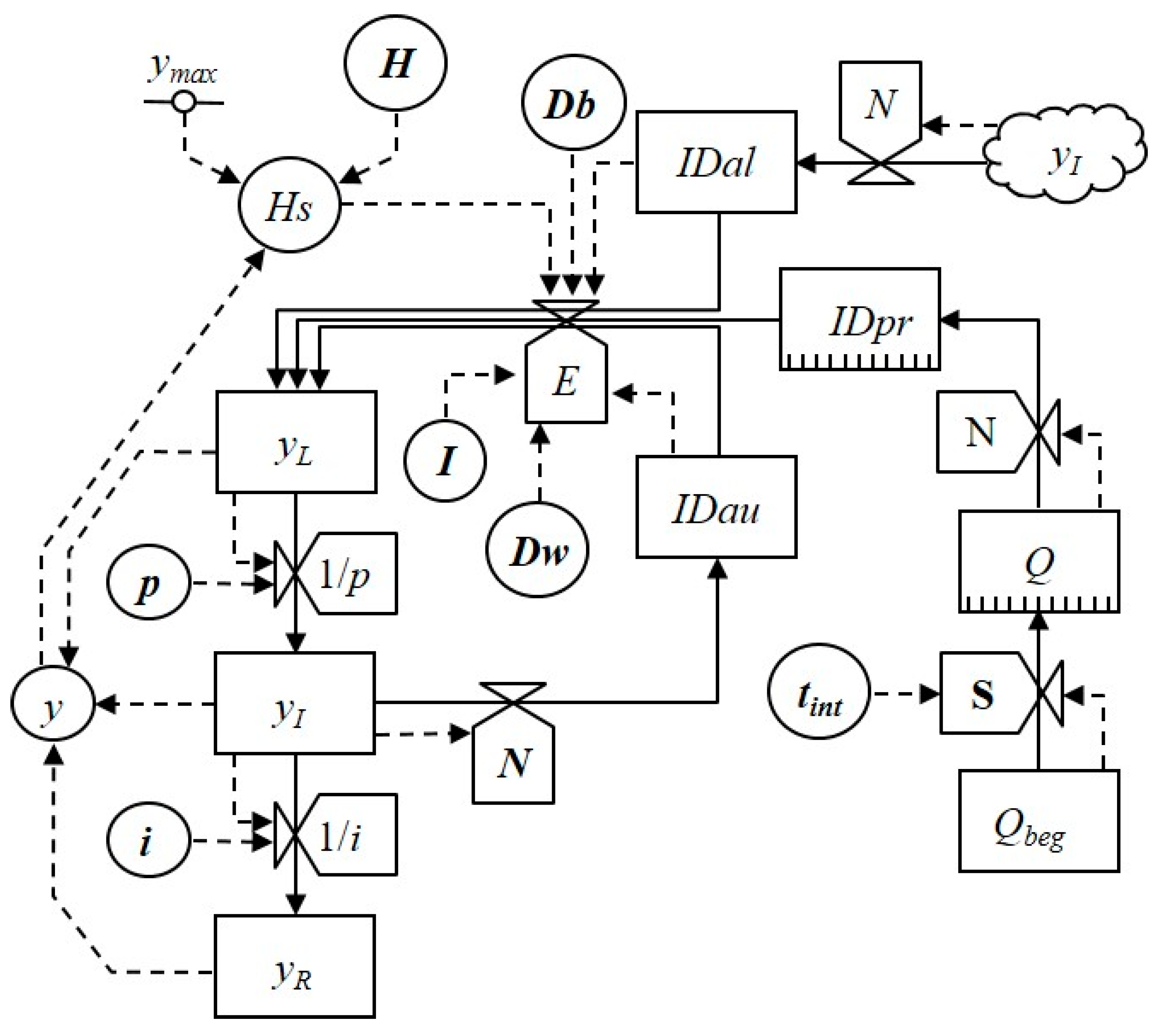
A relational diagram of the model is presented in Figure 1. The diagram has the following elements: (i) state variables, (ii) flows by which state variables change; (iii) rate variables, and (iv) parameters and intermediate variables. State variables include the proportion of affected host tissue (latent yL, infectious yI, and no longer infectious yR); overwintering inoculum (Q or Qbeg); and inoculum density (in primary inoculum, IDpr, secondary auto-inoculum, IDau, or secondary allo-inoculum, IDal). Rates variables include changes in latency (1/p) and infectiousness (1/i), relative proportion of spore production (N), infection effectiveness (E), and inoculum survival (S). Parameters and intermediate variables include duration of latency (p) and infectiousness (i), dispersal (Dw or Db), infection efficiency (I), time interval between crops (tint), actual (y) and maximum disease level (ymax), and relative amount of host tissue (H). In Figure 1, rates and intermediate variables affected by disease management actions are in bold.
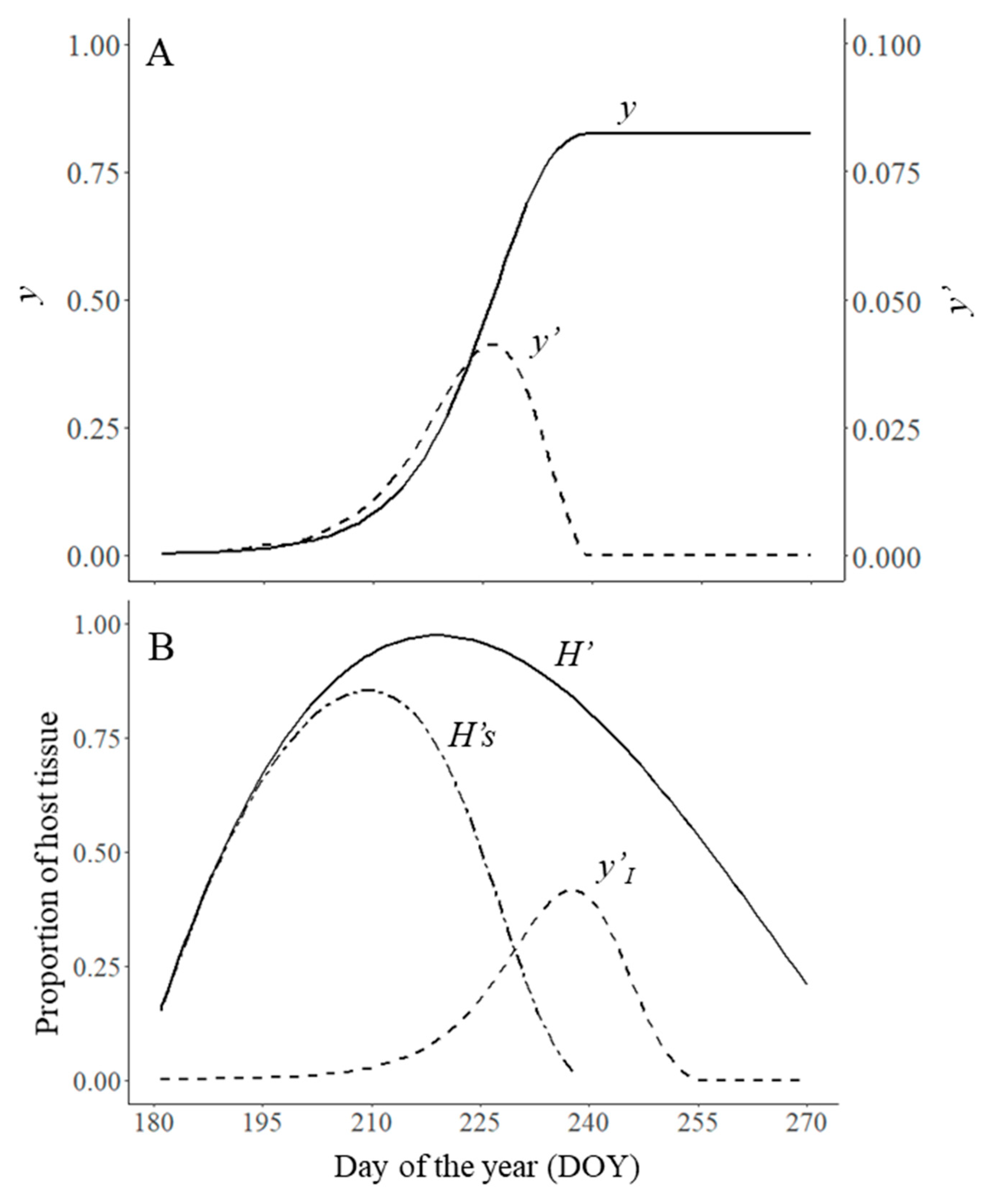
In this work, we operated the model using plausible parameter values for Cercoscopa beticola, causing Cercospora Leaf Spot (CLS) on sugar beet, as an example. Parametrization was based on the literature [25,26,27,28,29,30]. The initial disease level was set at 0.3% of affected leaf area (i.e., y0 = 0.003). The beginning of the epidemic was set on June 29 (t0 = 181 DOY), and the epidemic end on 26 September (te = 270 DOY). The maximum level of disease intensity (ymax) was set at 1, because CLS can completely destroy the plant canopy. The relative proportion of spore production (N) was set at 0.8, and proportion of spore that disperse within the crop (Dw) was 0.7 and between crops (Db) was 0, under the assumption that no spores are coming in from other sugar beet crops. The infection efficiency of the spores (I) was set at 0.8, the latent period (p) was 6 days, and the infectious period (i) was 12 days. The daily increase of the plant canopy was described by a beta equation of Analytis [31] in the form where x is the equivalent of the day of the year (DOY) in the form . The output of the model for this parametrization is shown in Figure 2. Afterward, we changed one or more model parameters in turn to simulate crop management actions. The resulting epidemics were then compared with the reference epidemic in terms of the final disease level (yf) and the area under the disease progress curve (AUDPC), calculated following Madden et al. [14]. The model was operated by using the software R v. 3.6.0 (R Foundation for Statistical Computing, Vienna, Austria) [32]; figures were plotted with the package ggplot2 [33].
3. Results
In this section, the model was used to simulate the effect of disease management actions on the epidemic dynamics.
3.1. Influence on the Initial Disease Level (y0)
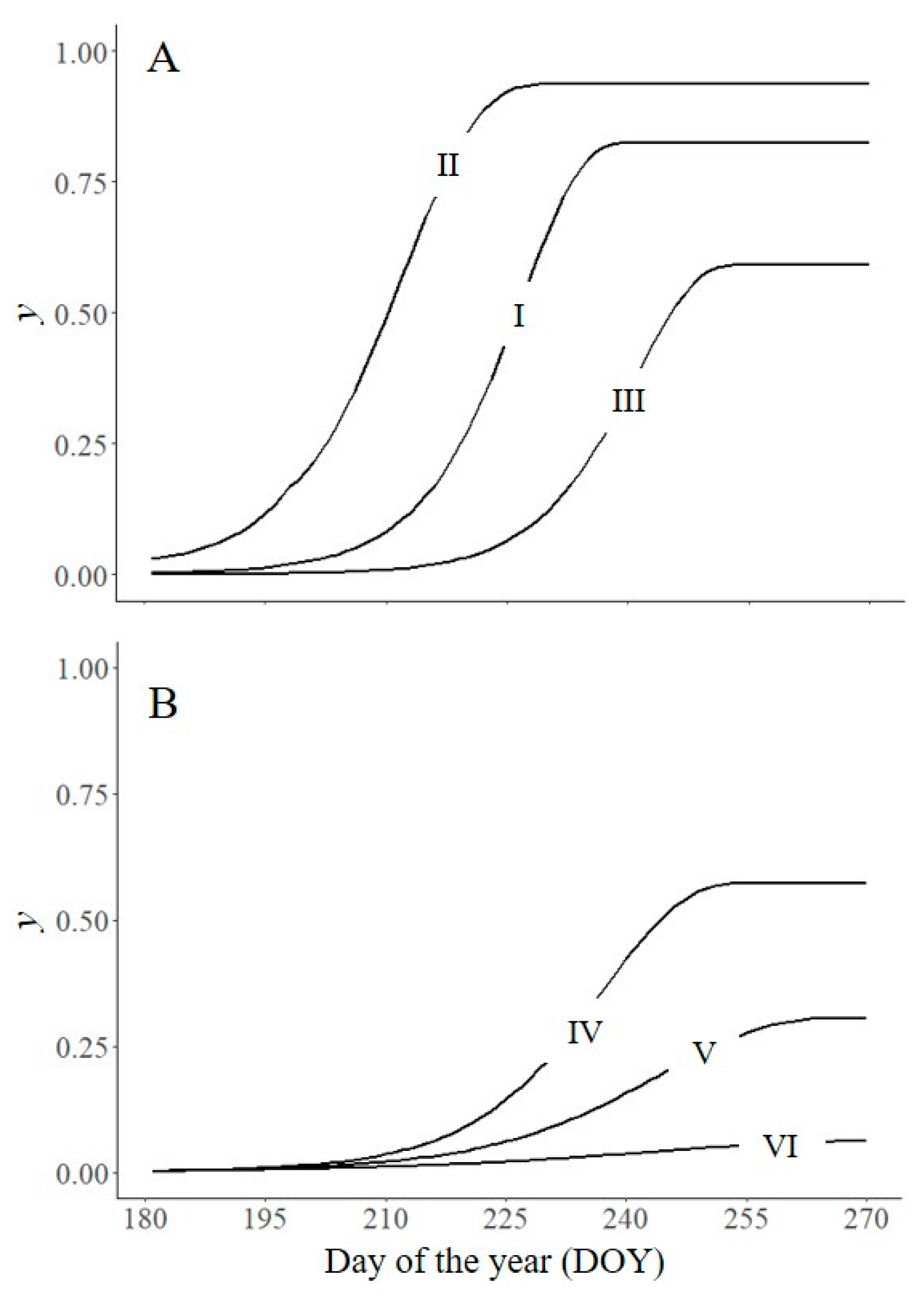
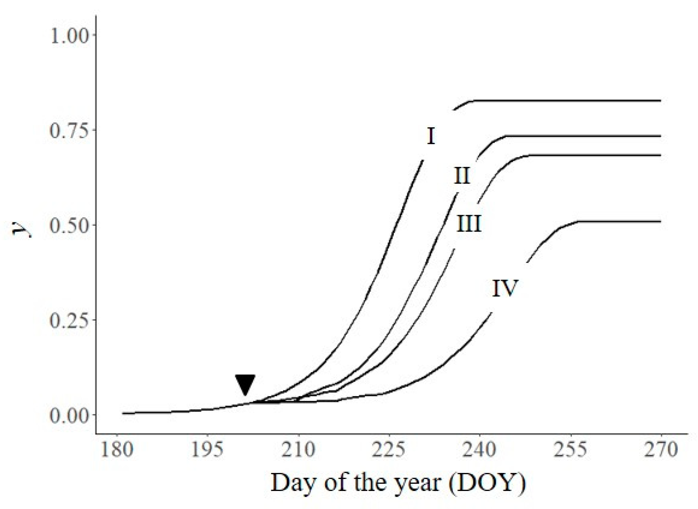
Sanitation includes measures aimed at excluding, eliminating, or reducing initial disease y0 [1,15]. Reducing y0 causes a delay in the epidemic. In Figure 3A, we operated the model by changing y0′. When y0′ was 0.03, yf was 0.94 and the AUDPC was 58.7; when y0′ was 10× or 100× smaller (0.003 and 0.0003, respectively), yf was 0.82 and 0.59, respectively, and the AUDPC was 39.6 and 20.1, respectively. These results indicate that the reduction in the epidemic measured as either final disease level or the AUDPC is less than the reduction in y0.
In epidemiological terms, sanitation influences y0 by influencing tint, S, Q, or D (Table 2). These influences are discussed in the following three paragraphs.
Exclusion prevents the pathogen from moving into a cropping area or into a crop. Exclusion reduces y0 by reducing Q or D. The pathogen can be excluded by (i) preventing the introduction and spread of pathogens into disease-free areas though policy-oriented regulation (quarantine, inspection, and certification); (ii) using pathogen-free propagating material (for those pathogens carried by seeds and vegetative propagating materials, like cuttings, root-stocks, tubers, etc.); (iii) growing the crop in greenhouses or plastic tunnels (for those pathogens entering the crop as air-borne spores); and (iv) preventing spores produced by resting forms in the soil from dispersing into the air with mulches of organic materials or plastic sheets (such mulches or sheets are chiefly used to conserve moisture and organic matter, reduce soil erosion, and control weeds) [34].
The initial inoculum can be reduced by reducing Q or S by (i) eliminating plant residues on the soil surface by ploughing (or raking, burning, or shredding), by treating residues with chemicals or biological control agents (BCAs), or by favouring residue decomposition; (ii) treating seeds or transplants with fungicides or chemical, physical, or biological control methods effective against seed-borne pathogens; and (iii) eliminating reservoirs for the overseasoning of fungi in affected plants. In perennial plants, reservoirs of inoculum are plant tissue (shoots with cankers, mummified fruits, etc.) that can be eliminated by pruning [9].
Initial inoculum can also be reduced by increasing the time interval between susceptible crops (tint) with crop rotation and crop-free periods. Increasing tint will reduce the survival S of the resting forms in the soil. A delay in the planting date similarly increases tint, but its effect is less than that of rotation because of the difference in time scales: months to years for rotation and only days to weeks for delayed planting.
3.2. Influence on the Rate of Disease Progress (y′)
Disease management actions aimed at reducing y′ will slow the epidemic. In Figure 3B, we operated the model as in Figure 3A but with different values for y′, including 1 (no disease control, line I in Figure 3A), 0.67, 0.50, or 0.33; the values were held constant for the entire duration of the epidemic. The resulting epidemics differed substantially in both yf (which declined with lower values of y′) and the AUDPC (which also declined with lower values of y′). Compared with no disease control, reducing y′ by 33%, 50%, and 67% reduced the AUDPC by 62%, 82%, and 96%, respectively.
Crop management actions influencing y′ are both strategic and tactical, are made at the farm and crop levels, and affect one or more of the following epidemiological components: H, p, i, N, D, and I (Table 3). These effects are discussed in the following sections.
3.2.1. Crop Growth and Development
Growth is the increase in size and weight of plants or plant parts, while development is the passing of the plant through successive, morphologically different stages [1]. Growth influences the volume H of the crop, while development influences its susceptibility to diseases (see Section 3.2.3).
Cropping practices that influence the amount of host tissue (H) directly affect disease progress because the quantity of host tissue available for infection determines the “carrying capacity” or maximum potential disease [35]. Cropping practices that influence the amount of host tissue (H) also indirectly affect disease progress because plants modify the environment, and the degree of modification is related to the quantity of plant tissue. Regarding the latter effect, changes in crop structure modify the microclimate of the crop, and these changes can benefit many fungi; the main changes involve vapour flux, with increased frequency, duration, and amount of dew covering plant surfaces as H increases [36].
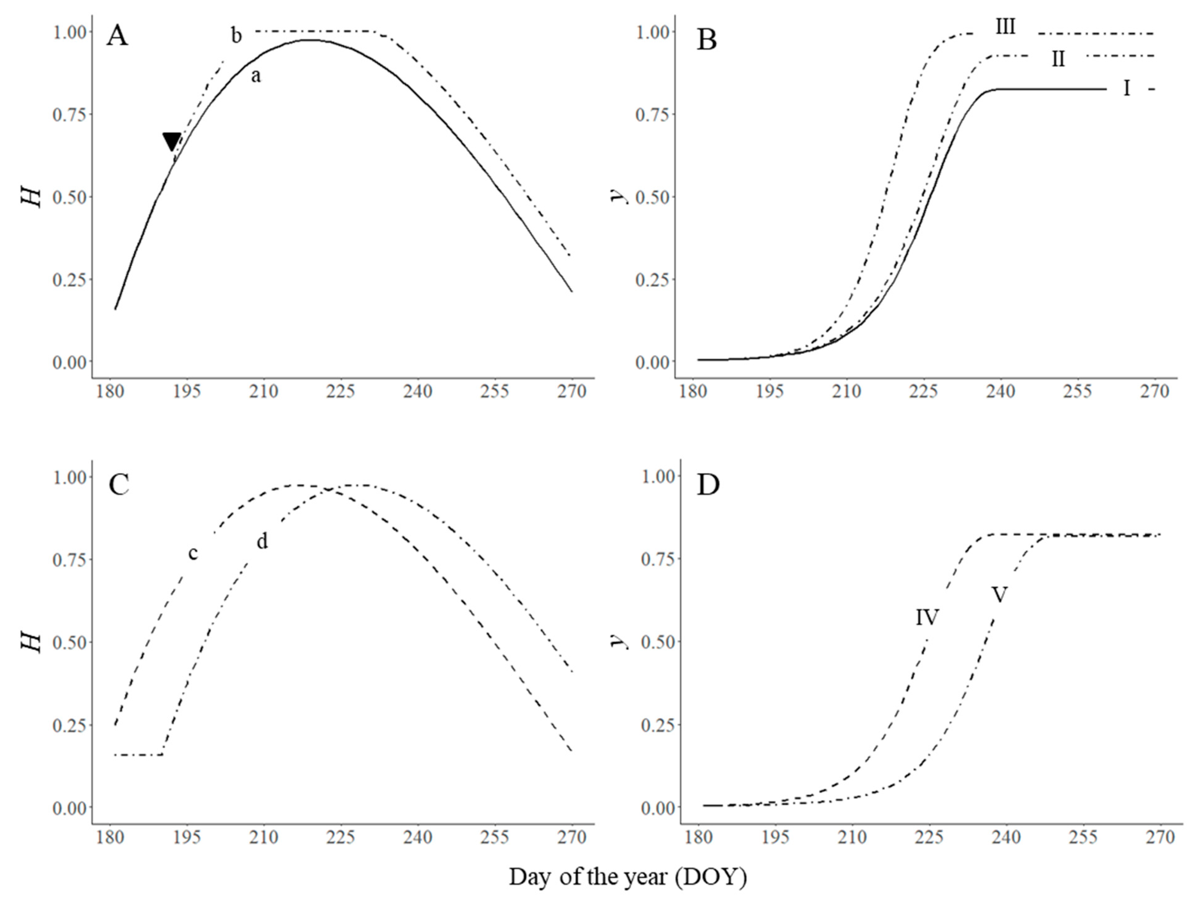
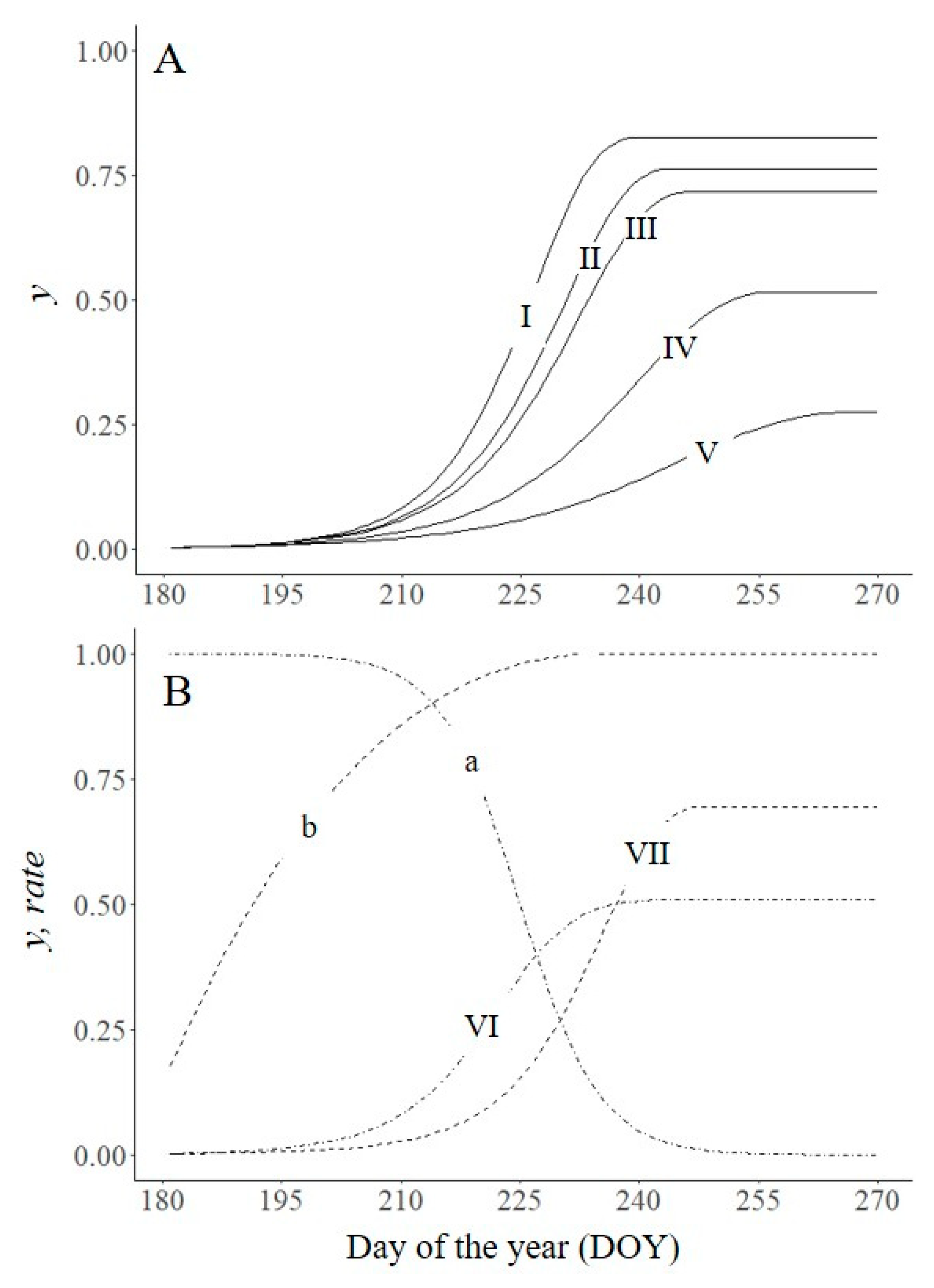
These direct and indirect effects are impossible to separate during natural epidemics, but they can be analysed separately by simulation. In Figure 4A,B, we operated the model in three ways: (i) as in Figure 2 (lines a and I); (ii) by increasing H′ by 10% from DOY 193 with no changes in other epidemiological components (lines b and II); and (iii) by changing those model parameters that can be affected by environmental changes due to increased H′, i.e., proportion of spore production, infection efficiency (N and I increased by 0.1), latent period (p shortened by 1 day), and infectious period (i lengthened by 2 days) (lines b and III). The increase in H′ (with no other changes) increased the final disease from 0.82 to 0.93 and the AUDPC from 39.6 to 44.7, while changes in both H and other epidemiological components increased the final disease to 1 and the AUDPC to 57.2.
Changes in H can also affect spore interception and thus the dispersal efficiency within the crop (Dw). As H increases, Dw will increase for air-borne spores because spores in a dense plant canopy have an increased probability of landing on a host surface rather than escaping through the upper crop boundary. The same can be expected for splash-borne spores, but in this case there is an opposite effect because of drop interception by upper canopy layers; an increase in H will reduce both the size and falling speed of raindrops that impact on sporulating host tissue [18].
Crop density can be manipulated directly (by sowing, pruning, thinning, trellising, staking, and harvesting some plants or plant parts) and indirectly by i) fertilization and irrigation, which increase the nutrient uptake from the soil, plant growth, biomass production, and ground coverage; ii) crop rotation, crop-free periods, and soil preparation, which enhance the agronomic characteristics of soil and also enhance plant growth; and iii) weed control, which reduces competition between crop plants and weeds (for space, light, water, and nutrients).
Cropping practices that affect the dynamics of the plant canopy (H′) also affect the disease epidemic. In Figure 4 (C and D), the model was used to simulate crop growth and epidemic progress with an early maturing variety (lines c and IV) and crop growth and epidemic progress with a late planting date (lines d and V), in comparison to the growth of the control (lines a and I in Figure 4A and B). yf was lower for the early variety than for the control (0.76 vs. 0.82), and the AUDPC was reduced by 31% compared to the control (27.5 vs. 39.6). A late planting date delayed the progress of the epidemic but produced similar values of yf as the control because the epidemic lasted longer.
Changes in H′ can result from (i) changes in planting date, (ii) use of plant varieties with life cycles of different lengths, (iii) fertilization, and (iv) irrigation, particularly when it is used to accelerate seed germination and plant emergence.
In addition to affecting H and H′, fertilization, irrigation, and weed control will have further effects on the disease [37,38,39,40]. With respect to fertilization, plant pathogens usually benefit from lush plant growth induced by abundant nitrogen uptake, because the nutrients supporting pathogen growth and reproduction are abundant in the plant tissue. This is particularly evident for biotrophic pathogens (like downy mildews, powdery mildews, and rusts). In contrast, weak pathogens benefit when nutrition for plant growth is poor.
Further effects of irrigation on disease include changes in sporulation, dispersal, and infection efficiency. These effects will vary with the kind of irrigation (subsoil, furrow, or sprinkler) and with the biology of the pathogen [40]. For instance, sprinkler irrigation greatly affects epiphytic fungal structures: water drops favour the dispersal of the splash-borne fungi (increase D), destroy colonies and conidiophores (reduce y and N), wash spores from air (increase D) and from plant surfaces (reduce I), and cause some kinds of spores (e.g., conidia of Erysiphaceae causing powdery mildews) to burst (reduce I). Irrigation also affects environmental conditions within the canopy by increasing the vertical flux of water from soil (all kinds of irrigation) and by wetting plant surfaces (sprinkler irrigation). This obviously increases N and I, and sometimes also increase i for the fungi favoured by a humid environment or by soaked tissues.
Further effects of weeds on disease include increases in total vegetation when weeds are not controlled. Furthermore, a dense weed canopy can intercept air- or splash-borne spores and thereby reduce Dw. Susceptible weeds can accommodate the pathogen and increase the density of spores available within the crop (ID). Finally, some herbicides inhibit pathogens and can contribute to disease control [39,41,42].
3.2.2. Fungicide Sprays and Other Tactical Actions against the Pathogen
Depending on their nature, chemical treatments against the pathogen have different epidemiological effects: protectant treatments prevent a plant from becoming infected; curative treatments kill the pathogen within the diseased host tissue (mainly during its latent stage); and eradicant treatments suppress sporulation and prevent secondary infections [43,44].
Both protectant and curative applications reduce I while the pathogen is on the host surface or soon after it penetrates the host tissue; curative fungicides can also increase p by interfering with pathogen growth within the host tissue. Eradicant treatments reduce N and probably i. Quantitative effects of chemicals in reducing y′ depend on their kill efficiency (or effectiveness) and its duration [45].
In Figure 5, the untreated control was compared with epidemics simulated by introducing a correction factor for I, i.e., a correction factor that accounted for the efficacy of the fungicide applied and the duration of its activity. The simulation used fungicide sprays that were applied at a disease threshold of 0.03 (on DOY 202) and that had different effectiveness (95 or 70%) and durations (7 or 14 days). With an effectiveness of 95%, yf fell from 0.82 (untreated, line I) to 0.73 when the fungicide remained active for 7 days (line II) and to 0.51 when the fungicide remained active for 14 days (line III); for the same parameter values, the AUDPC was 39.6, 31.1, and 16.6, respectively. When the effectiveness was 70% for 14 days (line IV), yf was 0.69 and the AUDPC was 27.7.
Treatments with BCAs are usually protectant [46]. The agents either antagonize or parasitize the pathogen on the host surface, or they occupy potential infection sites [47]. BCAs, therefore, influence I, N, and i [48].
Removal of host tissues infected by or suspected of harbouring the pathogen [9] excludes sources of inoculum for secondary infections. Removal of this tissue therefore reduces IDau by reducing i and N, and also IDal, when the removal is done at the farm or agro-system level. The latter is the case for eradication actions made compulsory by law ordinances against quarantined pathogens.
3.2.3. Plant Resistance
Resistance of the host plant greatly affects disease development [49]. Plant varieties with “vertical” resistance (VR) against the pathogen [50] reduce y0 by reducing the infection efficiency I of spores. This resistance occurs when host reactions block infection because the pathogen genotype lacks virulence genes to match the resistance genes of the host [51]. The degree of reduction in initial disease due to VR depends on the frequency of virulent vs. avirulent individuals in the geographic area.
As VR tends to be annulled in a few years by new virulent races of the pathogen, strategies are often applied at the farm and regional level to manage VR genes [52,53]. These include (i) pyramiding (i.e., accumulation of many vertical genes in one variety); (ii) regional deployment of genes (so that in a region prevails some genes that do not prevail in others); (iii) rotation of genes; and (iv) within-field mixture of vertical genes by cultivar mixtures and multi-line varieties. All of these strategies affect I by reducing the frequency of spores able to infect the crop plants during the primary inoculum season, i.e., by reducing the frequency of virulent genotypes. Use of cultivar mixtures also reduces D (see 3.2.4).
In contrast to plant varieties with VR, varieties with “horizontal” resistance (HR) [50] are effective against all individuals of a pathogen population; from a genetic point of view, HR includes multiple mechanisms and genetic patterns [51]. In quantitative epidemiology, HR can be regarded as a rate-reducing resistance in which the reduced disease level results from some interacting resistance components [54], each of them influencing epidemic components. HR varieties increase p and reduce i, I, and N. How HR varieties affect p, i, I, and N varies with the genetic backgrounds of the varieties [55,56,57].
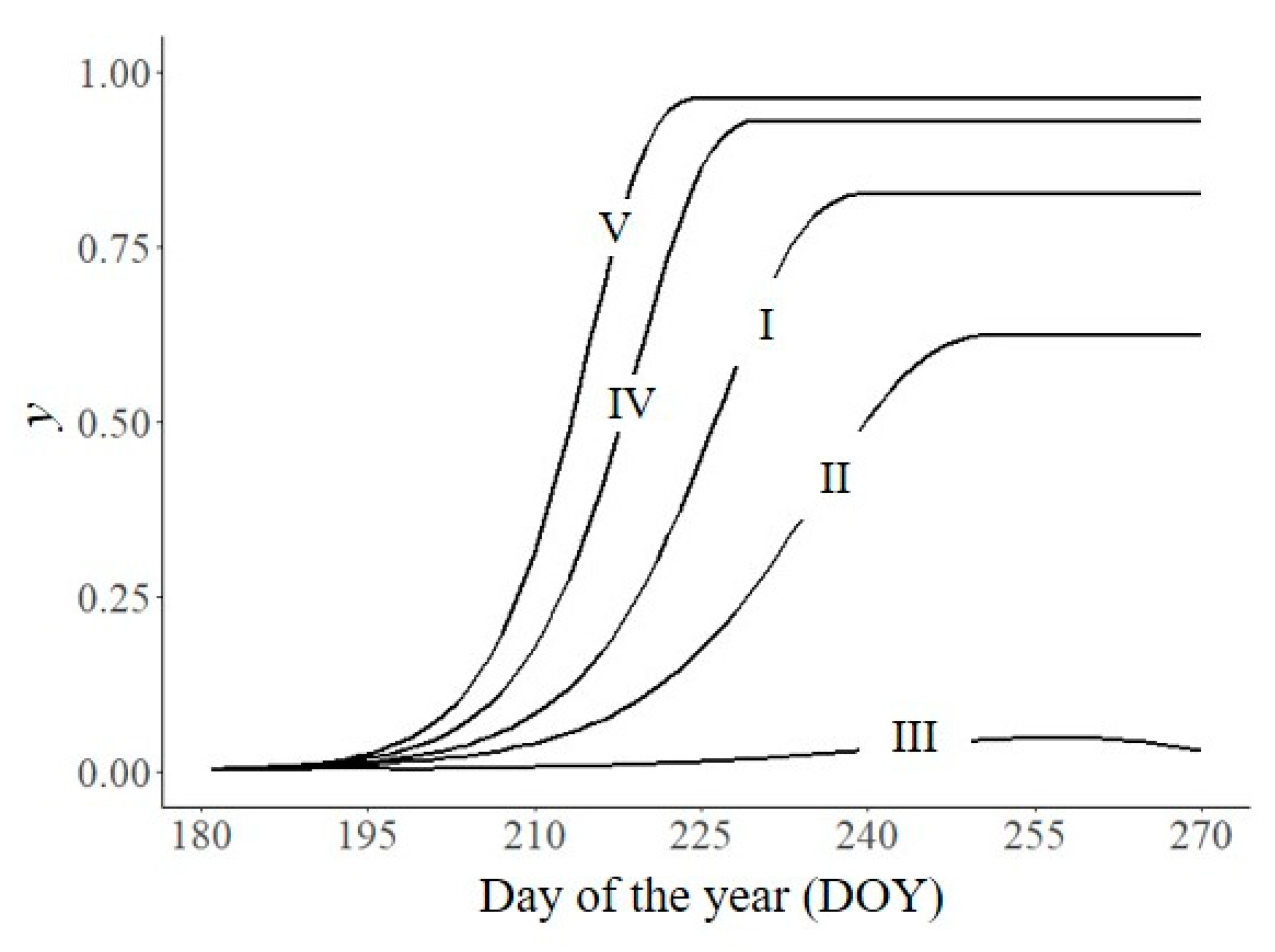
Empirically measuring the effect of each resistance component on the epidemic development is possible only by performing monocyclic experiments under environmentally controlled experiments, because the overlapping of infection cycles in natural epidemics makes such determinations impossible. For understanding natural epidemics, modelling enables simulation of the effect of each component on epidemiological processes as the epidemic progresses [58,59,60]. In Figure 6A, the model parameters were initially set as in Figure 2 to simulate a susceptible variety and were progressively changed to mimic the single and combined effects of an HR variety, in which p = 8, i = 10, N = 0.6, and I = 0.6. Final disease was reduced from 0.82 (line I) to 0.74 (line II), 0.68 (line III), 0.46 (line IV), and 0.22 (line V), respectively, while the AUDPC changed from 39.6 to 33.1, 29.1, 16.9, and 7.5, respectively.
Plants can be induced to switch on defense reactions to pathogens as a result of prior exposure to pathogens or to various stresses including chemicals and some BCAs [61,62]. Resistance resulting from such exposure or stress confers quantitative protection against a broad spectrum of microorganisms [63], and its epidemiological effects are similar to those of HR [64,65].
As mentioned in Section 3.2.1, plant reaction to disease changes with plant age, but the pattern of change differs among plants and pathogens [9]. In some pathosystems (e.g., downy mildews), plant tissues are susceptible only in the early growth stages and become resistant with aging (ontogenic resistance); in others, hosts become susceptible only after they reach maturity, and susceptibility increases with senescence (e.g., B. cinerea or Monilinia spp. affecting fruits). Therefore, depending on the particular host–pathogen combination, the host development stage at the time of arrival of the pathogen may greatly affect the epidemic [9].
In Figure 6B, the model simulated modifications of host susceptibility with age by using an index of susceptibility, which changed over the time of the epidemic between 1 (fully susceptible) and 0 (resistant). This index was multiplied by I, and the resulting epidemics (lines VI and VII, respectively) were compared with the control (line I, Figure 6A) in which the plants are susceptible over the entire epidemic. Obviously, both yf (0.51 and 0.67, respectively) and the AUDPC (26.1 and 27.6, respectively) were reduced in the plants that experienced changes of susceptibility with age (i.e., ontogenic resistance).
3.2.4. Aggregation of Plants and Crops
Aggregation is the degree to which plants and crops are grouped together [1]. Plant density, genotype mixture, multi-line varieties, and intercropping are examples of aggregation. The effects of these kinds of aggregation are discussed in the following paragraphs.
Plant density is the number of plants per unit of ground area. In plant epidemiology, plant density must be considered also as the level of within-field aggregation between host plants at both intraspecific and interspecific levels [66]. The highest level of aggregation is represented by a pure crop of genetically uniform plants; in this case, the effect of plant density is mainly related to H and consequently to Dw, as previously described.
Intraspecific within-field diversity due to genotype mixture and multi-line varieties influences not only y0, as previously mentioned, but also y′. Mixtures reduce the rate of disease progress by eliminating large numbers of spores at each cycle of the pathogen multiplication. Spores are eliminated from the epidemic process by deposition on plants carrying resistance genes and by dilution because of the greater distance between plants of the same genotype. Moreover, the infection process may be slowed by the induction of defence responses in susceptible plants elicited by the pathogen strains that are avirulent on specific host genotypes [66,67,68].
Interspecific diversity refers to the intercropping of different plant species in the same field. Intercropping is uncommon in conventional farming systems but is common and important in developing countries as well as in intensively managed horticultural and organic farms [40,69]. Intercropping can be obtained by mixing crops or by alternating rows of one crop with rows of another crop. From an epidemiological perspective [70], intercropping reduces H (expressed as susceptible host tissue per land surface unit) and Dw, because some spores are intercepted by the non-host plants. Disease reduction by intercropping partly depends on the combination of crop plants chosen, because some combinations can actually make disease worse by providing an alternate host or a stimulus that encourages germination of inoculum on the neighbouring species.
The within-crop dispersal proportion Dw is the main epidemiological component affected by within-field aggregation of plants. In Figure 7, the model was used to simulate the effect of reduced Dw; two dispersal proportions (0.5 and 0.3) were compared with that set in Figure 2 (0.7). Final disease was reduced from 0.8 (line I) to 0.62 (line II) and 0.18 (line III), respectively, whereas the AUDPC was reduced from 39.6 to 25.4 and 6.1, respectively.
Crop rotation, fallows, and crop-free periods influence the degree of between-field aggregation. Shortening of rotations increases spatial aggregation between fields in the same farm and thus reduces distances between crops. The main epidemiological consequence on y′ is an increase in the density of allo-inoculum that enters the crop area (increase in IDal). As spore deposition decreases exponentially with distance from the source [18], Db and IDal exponentially increase with reduced distance between crops.
In Figure 7, the model was used to simulate the effect of proximity of the crops. The model was operated as in Figure 2 and with the assumption that in the same area the epidemics progress in the same way in all the crops; in line I, the crop is isolated and therefore without ingression of allo-inoculum (Db = 0), while in lines IV and V, spores produced in other crops reach crop plants with a Db of 0.3 and 0.6, respectively. As a consequence, final disease increased from 0.82 to 0.93 and 0.96, respectively, while the AUDPC increased from 39.6 to 50.9 and 56.5, respectively.
3.3. Influence of Disease Management on the Duration of the Epidemic
Some cropping practices influence the disease by changing the duration of the epidemic (tepi). Obviously, a late start or an early end of the epidemic may reduce the disease. The crop management actions influencing the duration of the epidemic include both strategic and tactical actions that affect one or more of the following epidemiological components: t0, te, and tepi (Table 4).
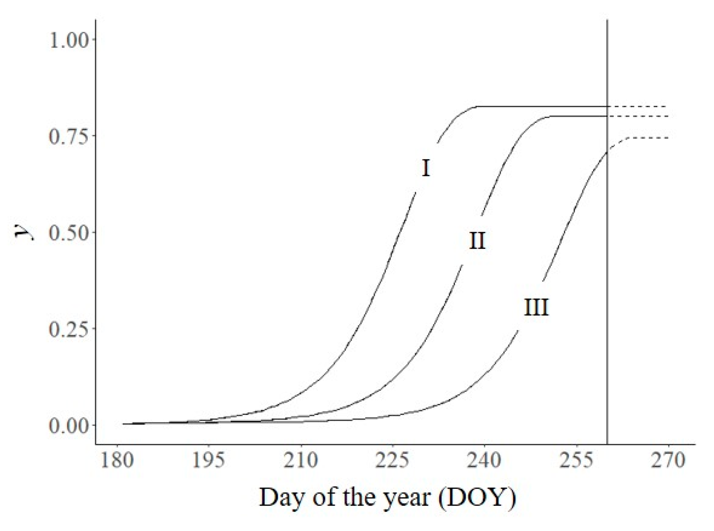
In Figure 8, the model was operated using the parameters set in Figure 2 and by changing t0 from 181 to 191 and 201. Final disease decreased by 0.03 and 0.13, respectively, while the AUDPC was reduced by 11 and 33%, respectively. With the same conditions, advancing harvest by 10 days (solid lines in Figure 8) the AUDPC decreased by 31 and 51%, respectively.
The duration of the epidemics can be reduced by harvesting at an earlier date, within the limits imposed by the crop physiology, whereas postponing t0 is difficult, because control measures against primary inoculum (see Section 3.1) influence y0 more than t0. In some cases, it seems that sanitation has delayed the onset of the first visible disease symptoms, but it is only an apparent effect, because a reduced y0 is difficult to detect by field inspection (i.e., the disease has appeared but the incidence value is so low that a rigorous inspection must be performed to detect symptoms). A change in t0 can be managed with cultural practices that modify the crop growth in the early growing season, because it advances or delays the time when dense canopies make the within-crop environmental conditions favourable for the pathogen. On the other hand, delaying t0 in a crop can increase y0 and IDal if neighbouring, more-developed crops are already affected.
Finally, in many crop plants, actions that increase plant growth can delay the time of physiological maturity and harvesting; by delaying te and lengthening tepi, these actions increase the final disease.
4. Discussion and Conclusions
The use of disease progress curves to characterize disease progress over time is essential for understanding how plant diseases develop and how disease control measures affect epidemics. To this purpose, Van der Plank in 1963 developed a model in which plant disease epidemics consisted of dynamic population processes with rates of change expressed in the form of nonlinear equations linked with control measures (with emphasis on disease resistance, chemical control, and inoculum reduction) [14]. Van der Plank represented the disease triangle (consisting of the host, the pathogen, and the environment) as equilateral, each side equivalent in its effects on disease development, and he called this “the equivalence theorem”. Van der Plank’s theorem or approach has been useful because the epidemiological parameters determining disease increase may be affected by variations in the host, the pathogen, and the environment, so that changes toward a more resistant host plant, a less aggressive pathogen, or a less favourable environment all have equivalent effects on the epidemic [35,71].
In the current work, a general and flexible model was developed that simulates progress over time of the epidemics caused by polycyclic fungal pathogens. The model, which is based on the logistic model proposed by Van der Plank’s [15], includes the effect of all crop management actions at different scales of complexity and all of the epidemiological parameters involved in the different stages of the pathogen life cycle. Nutter [34] emphasized that successful plant disease models must consider the initial inoculum (y0), infection rate (r), and period of time (t) that the pathogen and host populations interact. These three epidemiological parameters are included in the present model in that the model considers between-season survival, production of primary inoculum, occurrence of primary infections, production of secondary inoculum, and concatenation of secondary infection cycles during the cropping season. The model also considers the influence of neighbouring crops (such as allo-inoculum) in order to analyse epidemics at the farm level.
Considerable advances have been made in recent years in plant disease models, and most of these advances involve the use of differential equations to describe the dynamics of susceptible, infected, and removed host tissue (SIR models) [72,73]. These models describe the population dynamics of plant diseases in detail, and their complexity can be increased by adding multi-year disease dynamics, dynamics of host growth and susceptibility, interactions with biocontrol agents, metapopulation dynamics, or the responses of pesticide-resistant subpopulations (see the review of Scherm et al. [73]). However, the ideas and approaches of Van der Plank still have a large influence on plant pathologists who study epidemics [14]. The logistic equation developed by Van der Plank for polycyclic diseases is still valid for quantification of epidemics, especially over single growing seasons [72]. A number of plant disease models have been based on the fundamental work of Van der Plank [15] and have been used to simulate disease development under changing epidemiological conditions [35,59,74]. As it is based on the approach of Van der Plank, the model developed here is easy to implement by researchers, teachers or students, increasing its educational value.
Based on the equivalence theorem, all of the effects of crop management actions were translated into variations in the epidemiological components of the model, and the model was used to quantitatively simulate the effect of these actions on epidemic development. In this way, the model accounts for the “disease tetrahedron” [1] that symbolizes the effect of human activities on the disease triangle: each of the three components of the pathosystem (host, pathogen, and environment) can be influenced by human actions. A similar approach was used by Zadoks and Schein ([1], Table 11.1) and Kranz ([45], Table 7.2), who indicated in a general way whether major control measures affect r and/or yo. Palti [75] increased the number of epidemiological components considered, including p, i, N, and the duration of host susceptibility.
In polycyclic diseases, the control actions aimed at reducing y0 or delaying t0 can shift the disease progress curve; those reducing y′ slow the disease progress, while those shortening te interrupt the epidemic. All of these actions reduce disease severity at harvest, but they differ in effectiveness, ease of implementation, and levels of organization in decision making.
Control of primary inoculum (i.e., sanitation) is generally less effective than reduction of disease progress, as shown by simulations in the present work. Control of primary inoculum also involves decisions at higher organization levels [34,76]. For example, decisions at the national or international level are required for quarantine and inspections. Similarly, decisions at the level of the entire agricultural region are required for actions aimed at sustaining or emphasizing particular crops or environment-saving cropping regimes (like integrated or organic cropping) or at eradicating potentially devastating pathogens. Some strategic actions involve the entire farm organisation. These strategic actions, which usually affect y′, include (i) choice of crop species and cultivars; (ii) choice of crop type (open field or protected cultivation, uniform, or intercropping, etc.) and rotational schemes; (iii) elimination of inoculum reservoirs, not only from inside the field but also from the entire farm; (iv) choice of times and types of soil preparation and of planting dates; and (v) choice of cropping methods lasting some years (like the training system and plant density in orchards) or requiring depreciation allowances for equipment (like equipment needed for sub-soil or sprinkler irrigation) [76].
Most control actions that reduce the progress of the epidemics are tactical. They include (i) fungicide sprays (application times, products, and dosages) or alternative methods aimed at the pathogen (like BCAs or eradication); and (ii) cultural practices that regulate crop growth and canopy density (like fertilization, irrigation times and rates, weed control, etc.) [76].
Strategic actions are usually more difficult to implement than tactical actions: the time scale of strategic actions is measured in years instead of weeks or days, and they are more frequently limited by concerns about profit and the market [6,76]. In fact, the best cropping action for controlling disease is frequently less profitable than alternative actions. This is the case, for instance, in the use of ploughing vs. minimum tillage for control of Fusarium head blight of wheat (ploughing gives better control but smaller profits [77]), or in the use of sugar beet cultivars resistant to vs. susceptible to Cercospora leaf spot (resistant cultivars give better control but smaller profits [78]). In other cases, the best choice for disease management conflicts with the market preferences; this is true, for example, for grapevine varieties with resistance against mildews [79].
Similar considerations may be required when there is a choice between the tactical use of chemicals, alternative methods (i.e., the use of BCA), and cultural practices to control epidemics [46]. Chemicals often have higher, more constant, and predictable effectiveness, and are often easier to apply [44,46]. Even though some tactical disease control actions can have spectacular effects on actual epidemics, strategic decisions made at the agro-system and farm levels have a higher impact on disease risk because they act on the pathogen population for a few to many years [6,76].
The model described here should be considered as conceptual, i.e., it enables the identification of problems by distinguishing causes from effects and by quantifying the effects of specific events on epidemic development. Conceptual models are usually constructed as representations of ecological processes and can lead to the development of complex simulations. Conceptual plant disease models have been developed previously, and have been reviewed by Savary [24], Donatelli et al. [80], Savary et al. [35], Maanen and Xu [59], and Jones et al. [81], but in few cases only these models consider the effect of management. Savary [24] provided a conceptual simulation modelling framework for the linkages between crop and disease management and provided some perspective of use with specific pathosystems as examples. Savary focused on epidemiological components (i.e., y0, r and t) and did not make explicit the effect of the different management options on the epidemic. Bregaglio and Donatelli [82] developed a model to simulate the dynamics of polycyclic fungal epidemics and crop–pathogen interactions as affected by fungicide application but no by other management actions; the model can be used to explore situations in which no reference data are available, and simulations were performed for Puccinia recondita on wheat and Magnaporthe oryzae on rice. The model described here is an improvement on these conceptual models in that it considers most of the management options available for growers.
Models accounting for the management of specific pathosystems have been previously developed. One of the first was included in EPIPRE (acronym formed from the words epidemiology, prediction and prevention), a system of supervised control of diseases and pests in wheat; the system included a model for yellow rust that includes the effect of cultivar resistance and fertilization in the quantification of yield loss [83]. Avelino et al. [84] modelled the effect of several cropping practices on coffee rust (Hemileia vastatrix) by means of a multiple correspondence analysis. Rossi et al. [85] developed a decision support system (DSS) to determine the influence of environmental and agronomic factors (including host species and variety, previous crop, and type of soil tillage before sowing) on Fusarium head blight incidence and mycotoxin risk in small grain cereal; the DSS was validated with an independent dataset. All of these systems are empirical (they were developed based on field data), which results in the following limitations [58]: (i) they provide low detail in describing the pathosystem; (ii) they are difficult to extrapolate to different locations or pathosystems; and (iii) they have structures that cannot be extended with new knowledge. The mechanistic model described here is flexible and can be adapted to specific pathosystems by considering in each case the most important epidemiological components and the most common management actions.
The model described here can help researchers, students and policy makers understand how their management decisions will affect plant disease epidemics at different scales of complexity, with particular attention to the management options commonly recommended under an IPM framework [76]. By providing information on the benefits of management actions, the model should improve disease management.
Author Contributions
Conceptualization and methodology: V.R. and F.S.; analysis: V.R. and E.G.-D.; resources: V.R. and G.F.; writing—original draft preparation: V.R. and F.S.; writing—review and editing: E.G.-D., G.F., and V.R.; and supervision: V.R. All authors have read and agree to the published version of the manuscript.
Funding
This research received no external funding.
Acknowledgments
This work has benefitted from the research carried out within the project AgroScenari funded by the Italian Ministry for Agriculture, Food and Forestry Policies (Section 3.2.1, Section 3.2.2 and Section 3.2.3).
Conflicts of Interest
The authors declare no conflict of interest.
Computer Code and Software
R code will be available under request to the authors.
References
- Zadoks, J.C.; Schein, R.D. Epidemiology and Plant Disease Management; Oxford University Press Inc.: New York, NY, USA, 1979; p. 427. [Google Scholar]
- Alexander, H.M. Disease in natural plant populations, communities, and ecosystems: Insights into ecological and evolutionary processes. Plant Dis. 2010, 94, 492–503. [Google Scholar] [CrossRef] [PubMed] [Green Version]
- Matson, P.A.; Parton, W.J.; Power, A.G.; Swift, M.J. Agricultural intensification and ecosystem properties. Science 1997, 277, 504–509. [Google Scholar] [CrossRef] [PubMed] [Green Version]
- Higley, L.G.; Peterson, R.K. Economic Decision Rules for IPM. In Integrated Pest Management Concepts, Tactics, Strategies and Case Studies; Radcliffe, E.B., Hutchison, W.D., Cancelado, R.E., Eds.; Cambridge University Press: New York, NY, USA, 2009; pp. 25–32. [Google Scholar]
- Rabbinge, R.; Rossing, W.A.H.; Van der Werf, W. Systems approaches in epidemiology and plant disease management. Neth. J. Plant Pathol. 1993, 99, 161–171. [Google Scholar] [CrossRef] [Green Version]
- Rossi, V.; Caffi, T.; Salinari, F. Helping farmers face the increasing complexity of decision-making for crop protection. Phytopathol. Mediterr. 2012, 51, 457–479. [Google Scholar]
- Conway, G.R. Pest and Pathogen Control: Strategic, Tactical, and Policy Models; John Wiley and Sons: New York, NY, USA, 1984; p. 488. [Google Scholar]
- Rabbinge, R.; de Wit, C.T. Systems, model and simulation. In Simulation and Systems Management in Crop Protection; Rabbinge, R., Ward, S.A., van Laar, H.H., Eds.; PUDOC: Wageningen, The Netherlands, 1989; pp. 3–15. [Google Scholar]
- Agrios, G. Plant Pathology, 5th ed.; Academic Press: New York, NY, USA, 2005; p. 952. [Google Scholar]
- Fresco, L.O. Cassava in Shifting Cultivation. A Systems Approach to Agricultural Technology Development in Africa; Royal Tropical Institute: Amsterdam, The Netherlands, 1986; p. 240. [Google Scholar]
- Watt, K.E.F. The Nature of Systems Analysis. In Systems Analysis in Ecology; Watt, K.E.F., Ed.; Academic Press: New York, NY, USA, 1966; pp. 1–14. [Google Scholar]
- Horn, D.J. IPM as Applied Ecology: The Biological Precepts. In Integrated Pest Management: Concepts, Tactics, Strategies and Case Studies; Radcliffe, E.B., Hutchison, W.D., Cancelado, R.E., Eds.; Cambridge University Press: New York, NY, USA, 2009; pp. 51–61. [Google Scholar]
- Campbell, C.L.; Madden, L.V. Introduction to Plant Disease Epidemiology; John Wiley & Sons.: New York, NY, USA, 1990; p. 532. [Google Scholar]
- Madden, L.V.; Hughes, G.; van den Bosch, F. The Study of Plant Disease Epidemics; The American Phytopathological Society: Saint Paul, MN, USA, 2007. [Google Scholar]
- Van der Plank, J.E. Plant Diseases: Epidemics and Control; Academic Press: New York, NY, USA, 1963; p. 342. [Google Scholar]
- Leffelaar, P.A.; Ferrari, T.J. Some Elements of Dynamic Simulation. In Simulation and Systems Management in Crop Protection; Rabbinge, R., Ward, S.A., van Laar, H.H., Eds.; PUDOC: Wageningen, The Netherlands, 1989; pp. 19–45. [Google Scholar]
- Fitt, B.D.L.; MacCartney, H.A. Spore Dispersal in Relation to Epidemics Models. In Plant Disease Epidemiology, Voloume 1. Population Dynamics and Management; Leonard, K.J., Fry, W.E., Eds.; Macmillan: New York, NY, USA, 1986; pp. 311–345. [Google Scholar]
- Aylor, D. Aerial Dispersal of Pollen and Spores; American Phytopathological Society Press: Saint Paul, MN, USA, 2017; p. 418. [Google Scholar]
- Van der Plank, J.E. Host-Pathogen Interactions in Plant Diseases; Academic Press: New York, NY, USA, 1982; p. 203. [Google Scholar]
- Kushalappa, A.C.; Ludwig, A. Calculation of apparent infection rate in plant disease: Development of a method to correct for host growth. Phytopathology 1982, 72, 1373–1377. [Google Scholar] [CrossRef]
- Rouse, D.I. Use of Crop Growth-Models to Predict the Effects of Disease. Annu. Rev. Phytopathol. 1988, 26, 183–201. [Google Scholar] [CrossRef]
- Seem, R.C. The Measurement and Analysis of the Effects of Crop Development on Epidemics. In Experimental Techniques in Plant Disease Epidemiology; Kranz, J., Rotem, J., Eds.; Springer: Berlin/Heidelberg, Germany; New York, NY, USA, 1988; pp. 51–68. [Google Scholar]
- Casadebaig, P.; Quesnel, G.; Langlais, M.; Faivre, R. A generic model to simulate air-borne diseases as a function of crop architecture. PLoS ONE 2012, 7. [Google Scholar] [CrossRef]
- Savary, S. The roots of crop health: Cropping practices and disease management. Food Secur. 2014, 6, 819–831. [Google Scholar] [CrossRef]
- Rossi, V.; Battilani, P. CERCOPRI: A forecasting model for primary infections of cercospora leaf spot of sugarbeet. EPPO Bull. 1991, 21, 527–531. [Google Scholar] [CrossRef]
- Rossi, V.; Battilani, P. A simulated model for Cercospora leaf spot epidemics on sugarbeet. Phytopathol. Mediterr. 1994, 33, 105–112. [Google Scholar]
- Rossi, V.; Battilani, P.; Chiusa, G.; Giosuè, S.; Languasco, L.; Racca, P. Components of rate-reducing resistance to cercospora leaf spot in sugar beet: Incubation length, infection efficiency, lesion size. J. Plant Pathol. 1999, 81, 25–35. [Google Scholar]
- Rossi, V.; Meriggi, P.; Biancerdi, E.; Rossi, F. Effect of Cercospora leaf spot on sugar beet growth, yield and quality. Adv. Sugar Beet Res. 2000, 2, 49–76. [Google Scholar]
- Vereijssen, J.; Schneider, J.H.M.; Jeger, M.J. Epidemiology of cercospora leaf spot on sugar beet: Modeling disease dynamics within and between individual plants. Phytopathology 2007, 97, 1550–1557. [Google Scholar] [CrossRef] [PubMed]
- Wolf, P.F.J.; Verreet, J.A. Factors affecting the onset of Cercospora leaf spot epidemics in sugar beet and establishment of disease-monitoring thresholds. Phytopathology 2005, 95, 269–274. [Google Scholar] [CrossRef] [Green Version]
- Analytis, S. Über die Relation zwischen biologischer Entwicklung und Temperatur bei phytopathogenen Pilzen. J. Phytopathol. 1977, 90, 64–76. [Google Scholar] [CrossRef]
- Team, R.C. R: A Language and Environment for Statistical Computing; R Foundation for Statistical Computing: Vienna, Austria, 2019; Available online: https://www.R-project.org/ (accessed on 4 February 2020).
- Wickham, H. ggplot2 Elegant Graphics for Data Analysis; Springer: New York, NY, USA, 2016. [Google Scholar]
- Nutter, F.W. The Role of Plant Disease Epidemiology in Developing Successful Integrated Disease Management Programs. In General Concepts in Integrated Pest and Disease Management; Ciancio, A., Mukerji, K.G., Eds.; Springer: Berlin/Heidelberg, Germany; New York, NY, USA, 2007; pp. 45–79. [Google Scholar]
- Savary, S.; Nelson, A.D.; Djurle, A.; Esker, P.D.; Sparks, A.; Amorim, L.; Bergamin Filho, A.; Caffi, T.; Castilla, N.; Garrett, K.; et al. Concepts, approaches, and avenues for modelling crop health and crop losses. Eur. J. Agron. 2018, 100, 4–18. [Google Scholar] [CrossRef]
- Ando, K.; Grumet, R.; Terpstra, K.; Kelly, J.D. Manipulation of plant architecture to enhance crop disease control. CAB Rev. Perspect. Agric. Vet. Sci. Nutr. Nat. Resour. 2007, 2, 1–8. [Google Scholar] [CrossRef]
- Rotem, J.; Palti, J. Irrigation and plant disease. Annu. Rev. Phytopathol. 1969, 7, 267–288. [Google Scholar] [CrossRef]
- Huber, D.M.; Watson, R.D. Nitrogen form and plant disease. Annu. Rev. Phytopathol. 1974, 12, 139–165. [Google Scholar] [CrossRef]
- Altman, J.; Campbell, C.L. Effect of herbicides on plant diseases. Annu. Rev. Phytopathol. 1977, 15, 361–385. [Google Scholar] [CrossRef]
- Van Bruggen, A.H.C.; Gamliel, A.; Finckh, M.R. Plant disease management in organic farming systems. Pest Manag. Sci. 2016, 72, 30–44. [Google Scholar] [CrossRef] [PubMed]
- Richardson, L.T. Effect of insecticides and herbicides applied to soil on the development of plant diseases. I. The seedling diseases of barley caused by Helminthosporium sativum P.K. and B. Can. J. Plant Pathol. 1957, 37, 196–204. [Google Scholar] [CrossRef] [Green Version]
- Manici, L.M.; Rossi, V. Study of biological activity in vitro of some herbicides against Pyricularia oryzae Briosi et Cavara and Drechslera oryzae Subr. et Jain. Ann. Fac. Agrar. Univ. Stud. Milan 1990, 30, 29–35. [Google Scholar]
- McGrath, M.T. What are Fungicides? Plant Health Instr. 2004. [Google Scholar] [CrossRef]
- Caffi, T.; Rossi, V. Fungicide models are key components of multiple modelling approaches for decision-making in crop protection. Phytopathol. Mediterr. 2018, 57, 153–169. [Google Scholar]
- Kranz, J. Comparative Epidemiology of Plant Diseases; Springer: Berlin/Heidelberg, Germany; New York, NY, USA, 2003; p. 590. [Google Scholar]
- Tamm, L.; Speiser, B.; Holb, I. Direct Control of Airborne Diseases. In Plant Diseases and Their Management in Organic Agriculture; Finckh, M.R., Bruggen, A.H.C., Tamm, L., Eds.; APS Press: St. Paul, MN, USA, 2015; pp. 205–216. [Google Scholar]
- Andrews, J.H. Biological control in the phyllosphere. Annu. Rev. Phytopathol. 1992, 30, 603–635. [Google Scholar] [CrossRef]
- Fedele, G.; Bove, F.; González-Domínguez, E.; Rossi, V. A generic model accounting for the interactions among pathogens, host plants, biocontrol agents, and the environment, with parametrization for Botrytis cinerea on grapevines. Agronomy 2020, 10, 222. [Google Scholar] [CrossRef] [Green Version]
- Welz, G.; Kranz, J. Effects of Resistance on the Development of Disease in Crops. In Resistance of Crop Plants Against Fungi; Hartleb, H., Heitefuβ, R., Hoppe, H.H., Eds.; Fischer: Jena, Germany, 1997. [Google Scholar]
- Van der Plank, J.E. Disease Resistance in Plants, 2nd ed.; Academic Press: New York, NY, USA, 1984; p. 191. [Google Scholar]
- Ribeiro do Vale, F.X.; Parlevliet, J.E.; Zambolim, L. Concepts in plant disease resistance. Fitopatol. Bras. 2001, 26, 577–589. [Google Scholar] [CrossRef]
- Mundt, C.C.; Cowger, C.; Garrett, K.A. Relevance of integrated disease management to resistance durability. Euphytica 2002, 124, 245–252. [Google Scholar] [CrossRef]
- Mundt, C.C. Durable resistance: A key to sustainable management of pathogens and pests. Infect. Genet. Evol. 2014, 27, 446–455. [Google Scholar] [CrossRef]
- Zadoks, J.C. Modern Concepts of Disease Resistance in Cereals. In Proceedings of the Way Ahead in Plant Breeding, Cambridge, MA, USA, 29 June–2 July 1972; pp. 89–98. [Google Scholar]
- Rossi, V. Effect of host resistance in decreasing infection rate of Cercospora leaf spot epidemics on sugarbeet. Phytopathol. Mediterr. 1995, 34, 149–156. [Google Scholar]
- Rossi, V. Cercospora leaf spot infection and resistance in sugar beet. Adv. Sugar Beet Res. 2000, 2, 17–48. [Google Scholar]
- Bove, F.; Rossi, V. Components of partial resistance to Plasmopara viticola enable complete phenotypic characterization of grapevine varieties. Sci. Rep. 2020, 10, 585. [Google Scholar] [CrossRef] [PubMed] [Green Version]
- Rossi, V.; Giosuè, S.; Caffi, T. Modelling Plant Diseases for Decision Making in Crop Protection. In Precision Crop Protection—The Challenge and Use of Heterogeneity; Oerke, E.C., Gerhards, R., Menz, G., Sikora, R.A., Eds.; Springer: Dordrecht, The Netherlands, 2010; pp. 241–258. [Google Scholar]
- Van Maanen, A.; Xu, X.M. Modelling plant disease epidemics. Eur. J. Plant Pathol. 2003, 109, 669–682. [Google Scholar] [CrossRef]
- Bove, F.; Savary, S.; Willocquet, L.; Rossi, V. Modelling the effect of partial resistance on epidemics of downy mildew of grapevine. Eur. J. Agron. 2020, submitted. [Google Scholar]
- Kessmann, H.; Staub, T.; Hofmann, C.; Maetzke, T.; Herzog, J.; Ward, E.; Uknes, S.; Ryals, J. Induction of Systemic Acquired Disease Resistance in Plants by Chemicals. Annu. Rev. Phytopathol. 1994, 32, 439–459. [Google Scholar] [CrossRef]
- Elad, Y.; Freeman, S. Biological Control of Fungal Plant Pathogens. In Agricultural Applications; Kempken, F., Ed.; Springer: Berlin/Heidelberg, Germany, 2002; pp. 93–109. [Google Scholar]
- Métraux, J.P.; Nawrath, C.; Genoud, T. Systemic acquired resistance. Euphytica 2002, 124, 237–243. [Google Scholar] [CrossRef]
- Jeger, M.J.; Jeffries, P.; Elad, Y.; Xu, X.M. A generic theoretical model for biological control of foliar plant diseases. J. Theor. Biol. 2009, 256, 201–214. [Google Scholar] [CrossRef]
- Xu, X.M.; Jeffries, P.; Pautasso, M.; Jeger, M.J. A numerical study of combined use of two biocontrol agents with different biocontrol mechanisms in controlling foliar pathogens. Phytopathology 2011, 101, 1032–1044. [Google Scholar] [CrossRef] [Green Version]
- Garrett, K.A.; Mundt, C.C. Epidemiology in mixed host populations. Phytopathology 1999, 89, 984–990. [Google Scholar] [CrossRef] [Green Version]
- Chin, K.M.; Wolfe, M.S. The spread oi Erysiphe graminis f. sp. hordei in mixtures of barley varieties. Plant Pathol. 1984, 33, 89–100. [Google Scholar] [CrossRef]
- Lannou, C.; De Vallavieille-Pope, C.; Goyeau, H. Induced resistance in host mixtures and its effect on disease control in computer-simulated epidemics. Plant Pathol. 1995, 44, 478–489. [Google Scholar] [CrossRef]
- Altieri, M.A.; Nicholls, C.I.; Ponti, L. Crop Diversification Strategies for Pest Regulation in IPM Systems. In Integrated Pest Management: Concepts, Tactics, Strategies and Case Studies; Radcliffe, E., Hutchison, W., Cancelado, R., Eds.; Cambridge University Press: Cambridge, UK, 2008; pp. 116–130. [Google Scholar]
- Trenbath, B.R. Intercropping for the management of pests and diseases. Field Crop. Res. 1993, 34, 381–405. [Google Scholar] [CrossRef]
- Berger, R.D. Application of Epidemiological Principles to Achieve Plant Disease Control. Annu. Rev. Phytopathol. 1977, 15, 165–181. [Google Scholar] [CrossRef]
- Madden, L.V. Botanical epidemiology: Some key advances and its continuing role in disease management. Eur. J. Plant Pathol. 2006, 115, 3–23. [Google Scholar] [CrossRef]
- Scherm, H.; Ngugi, H.K.; Ojiambo, P.S. Trends in theoretical plant epidemiology. Eur. J. Plant Pathol. 2006, 115, 61–73. [Google Scholar] [CrossRef]
- Zadoks, J.C. Systems analysis and the dynamics of epidemics. Phytopathology 1971, 61, 600–610. [Google Scholar]
- Palti, J. Cultural Practices and Infectious Crop Diseases; Springer: Berlin/Heidelberg, Germany; New York, NY, USA, 1981; p. 246. [Google Scholar]
- Rossi, V.; Sperandio, G.; Caffi, T.; Simonetto, A.; Gilioli, G. Critical success factors for the adoption of decision tools in IPM. Agronomy 2019, 9, 710. [Google Scholar] [CrossRef] [Green Version]
- Rossi, V.; Delogu, G.; Giosuè, S.; Scudellari, D. Influence of the Cropping System on Fusarium Mycotoxins in Wheat Kernels. In Proceedings of the 2nd International Symposium on Fusarium Head Blight, Orlando, FL, USA, 11–15 December 2004; pp. 498–501. [Google Scholar]
- Rossi, V.; Battilani, P.; Chiusa, G.; Giosuè, S.; Languasco, L.; Racca, P. Components of rate-reducing resistance to cercospora leaf spot in sugar beet: Conidiation length, spore yield. J. Plant Pathol. 2000, 82, 125–131. [Google Scholar]
- Gessler, C.; Pertot, I.; Perazzolli, M. Plasmopara viticola: A review of knowledge on downy mildew of grapevine and effective disease management. Phytopathol. Mediterr. 2011, 50, 3–44. [Google Scholar]
- Donatelli, M.; Magarey, R.D.; Bregaglio, S.; Willocquet, L.; Whish, J.P.M.; Savary, S. Modelling the impacts of pests and diseases on agricultural systems. Agric. Syst. 2017, 155, 213–224. [Google Scholar] [CrossRef] [PubMed]
- Jones, J.W.; Antle, J.M.; Basso, B.; Boote, K.J.; Conant, R.T.; Foster, I.; Godfray, H.C.J.; Herrero, M.; Howitt, R.E.; Janssen, S.; et al. Brief history of agricultural systems modeling. Agric. Syst. 2017, 155, 240–254. [Google Scholar] [CrossRef] [PubMed]
- Bregaglio, S.; Donatelli, M. A set of software components for the simulation of plant airborne diseases. Environ. Model. Softw. 2015, 72, 426–444. [Google Scholar] [CrossRef]
- Zadoks, J.C.; Rijsdijk, F.; Rabbinge, R. EPIPRE, A Systems Approach to Supervised Control of Pests and Diseases of Wheat in The Netherlands. In Pest and Pathogen Conrol: Strategic, Tactical and Policy Models; Conway, G.R., Ed.; Wiley: New York, NY, USA, 1984; pp. 344–351. [Google Scholar]
- Avelino, J.; Willocquet, L.; Savary, S. Effects of crop management patterns on coffee rust epidemics. Plant Pathol. 2004, 53, 541–547. [Google Scholar] [CrossRef]
- Rossi, V.; Giosuè, S.; Terzi, V.; Scudellari, D. A decision support system for Fusarium head blight on small grain cereals. EPPO Bull. 2007, 37, 359–367. [Google Scholar] [CrossRef]
Figure 1.
Relational diagram of the model simulating plant disease epidemics. The diagram is drawn following Leffelaar and Ferrari [16]: boxes are state variables, valves are rates, circles are intermediate variables, the dotted line is a constant, arrows with solid lines indicate flows and directions by which state variables change, and arrows with dotted lines indicate flows of information. Symbols are listed in Table 1. The variables affected by changes in crop management actions are in bold.

Figure 2.
(A) Temporal dynamics of total (y) and relative (y′) disease; (B) daily increase in the host tissue (H′), tissue free from infection (H′s), and sporulating diseased tissue (y′I). Values were obtained by running the model using parameters values for Cercospora Leaf Spot of sugar beet: y0′ = 0.003, t0 = 181, te = 270, ymax = 1, N = 0.8, Dw = 0.7, Db = 0, I = 0.8, p = 6, i = 12, and , being x is the equivalent of the day of the year (DOY) in the form x = (DOY − 170)/(280 − 170). Symbols are listed in Table 1.

Figure 3.
Effect of crop management actions that affect either y′0 (A) or y′ (B) on disease intensity (y). I: untreated control, y0′ = 0.003, y′ as in Figure 2; II: y0′ = 0.03; III: y0′ = 0.0003; IV: y′ as in Figure 2 times 0.67; V: y′ as in Figure 2 times 0.5; and VI: y′ as in Figure 2 times 0.33. Symbols are listed in Table 1.

Figure 4.
Effect of changes in plant growth (H ; A,C) on disease severity (y; B,D). (A) a: H′ as in Figure 2: , being x is the equivalent of the day of the year (DOY) in the form x = (DOY − 170)/(280 − 170); b: H′ increased beginning with DOY 193 (▼). (B) I: untreated control as in Figure 2 (N = 0.8, I = 0.8, p = 6, i = 12, H′ = a); II: epidemic for H′ = b; III: H′ = b and model parameters change to N = 0.9, I = 0.9, p = 5, i = 14. (C) c: H′ modified by sowing a short-cycle plant variety; d: H′ modified by delaying sowing date. (D) IV: epidemic for H′ = c; V: epidemic for H′ = d. Symbols are listed in Table 1.

Figure 5.
Effect on disease severity (y) of one treatment with protectant fungicides applied on DOY 202 (▼). I: untreated control, as in Figure 2; II: efficacy of 95% for 7 days; III: efficacy of 95% for 14 days; IV: efficacy of 70% for 14 days. Symbols are listed in Table 1.

Figure 6.
Effect on disease severity (y) of changes in plant resistance, either as horizontal (A) or ontogenic (B) resistance. I: control (susceptible plant), as in Figure 2 (N = 0.8, I = 0.8, p = 6, i = 12); II, resistance due to increased latent period (N = 0.8, I = 0.8, p = 8, i = 12); III, resistance due to reduced infectious period (N = 0.8, I = 0.8, p = 8, i = 10); IV, resistance due to reduced sporulation (N = 0.6, I = 0.8, p = 8, i = 10); V, resistance due to reduced infection efficiency (N = 0.6, I = 0.6, p = 8, i = 10); VI: plant susceptibility decreased by age; VII: plant susceptibility increased by age; lines a and b are relative rates of susceptibility for lines VI and VII, respectively. Symbols are listed in Table 1.

Figure 7.
Effect on disease severity (y) of spatial aggregation between host plants. I: control, as in Figure 2 (Dw = 0.7, Db = 0); II and III, reduced within-crop aggregation due to cultivar mixture: II, Dw = 0.5, Db = 0; III, Dw = 0.3, Db = 0; IV and V, increased between-field aggregation due to shortened crop rotation: IV, Dw = 0.7, Db = 0.3; V, Dw = 0.7, Db = 0.6. Symbols are listed in Table 1.

Figure 8.
Effect on disease severity (y) of changing times when the disease epidemic begins. I: control, as in Figure 2 (t0 = 181, te = 270); II: t0 = 191, te = 270 (---) or 260 (—); III: t0 = 201, te = 270 (---) or 260 (—). A vertical solid line marks the advance of 10 days of harvest (i.e., te = 260 instead of 270). Symbols are listed in Table 1.


Table 1.
List of symbols used in the model.
| Symbol | Description and Dimension |
|---|---|
| D | Proportion of spores that disperse, within the crop (Dw) or between crops (Db) (T−1) a |
| E | Effectiveness of spores in causing new infections (T−1) |
| H | Total plant tissue (P) b |
| Hs | Plant tissue that can be infected (P) |
| H′ | Daily increase of H (T−1) |
| i | Infectious period (T, in days) |
| I | Infection efficiency of spores (T−1) |
| ID | Inoculum density: primary inoculum (IDpr); secondary inoculum, produced inside (auto-inoculum, IDau) or outside (allo-inoculum, IDal) the crop (N·L−2) |
| N | Relative proportion of spore production by inoculum sources (T−1) |
| p | Latent period (T, in days) |
| Q | Density of resting forms at the beginning of the survival period (Qbeg), or at any time t during the primary season (Qt) (n) c |
| r | Apparent infection rate (T−1) |
| S | Proportion of resting forms that survive (T−1) |
| t | Time (T) |
| t0 | Time at which first seasonal infection occurs (T, DOY) d |
| t00 | Time when resting forms are produced by previous epidemic (T, DOY) |
| te | Time when the epidemic ends (natural end or crop harvest) (T, DOY) |
| tepi | Total duration of the epidemic, time between t0 and te (T, weeks or months) |
| tint | Time interval between t00 and t0 (T, months or years) |
| tp | Time when there is no more primary inoculum (T, DOY) |
| y0 | Initial disease level (P) |
| y′0 | Daily increase of y0 (T−1) |
| yf | Final disease level (P) |
| ymax | Maximum plant tissue that can became diseased (P) |
| yt | Total disease level at time t (includes latent, infectious, and removed tissue) (P) |
| y′ | Daily increase of y (T−1) |
| yt −yt − p | Diseased tissue that is into the latent period by time t (yL)(P) |
| yt – I − p | Diseased tissue that had passed through the latent and infectious period by time t (removed or post-infectious diseased tissue) (yR) (P) |
| yt − p | Diseased tissue that had passed through the latent period by time t (P) |
| yt − p -yt – I − p | Infectious (sporulating) diseased tissue (yI) (P) |
a T = time (in days), b P = proportion of the plant surface (0 to 1), c n = number, d DOY = day of the year.
Table 2.
Main effects of crop management actions on increasing (+) or reducing (−) epidemiological parameters that affect the disease level at the beginning of the epidemic.
Table 2.
Main effects of crop management actions on increasing (+) or reducing (−) epidemiological parameters that affect the disease level at the beginning of the epidemic.
| Crop Management Action | tint a | S | Q | D | I | y0 |
|---|---|---|---|---|---|---|
| Strategic | ||||||
| Biological control agents | − | − | ||||
| Crop rotation (long) | + | − | ||||
| Crop-free periods | + | − | ||||
| Mixture of plant varieties | − | − | − | |||
| Elimination of plant residues | − | − | ||||
| Elimination of inoculum reservoirs | − | − | ||||
| Mulching | − | − | ||||
| Pathogen-free propagation material | − | − | ||||
| Sanitation of seeds/transplants | − | − | ||||
| Soil disinfestation | − | − | ||||
| Sowing/planting date (postponing) | + | − | ||||
| Spatial isolation between plants/crops | − | − | ||||
| Soil tillage | +/−b | +/− | ||||
| Plant resistance | − | − |
a Symbols are listed in Table 1, b+/− = the effect depends on the pathosystem.
Table 3.
Main effects of crop management actions on increasing (+) or reducing (−) epidemiological parameters that affect the rate of epidemic progress.
Table 3.
Main effects of crop management actions on increasing (+) or reducing (−) epidemiological parameters that affect the rate of epidemic progress.
| Crop Management Action | Ha | H′ | p | i | N | Dw | Db | I | y′ |
|---|---|---|---|---|---|---|---|---|---|
| Tactical | |||||||||
| Biological control agents | − | − | |||||||
| Canopy density (increase) | + | (−) b | (+) | (+) | +/−c | (+) | +/− | ||
| Eradication | − | − | − | ||||||
| Fertilization | + | /d | (−) | (+) | (+) | (+) | + | ||
| Fungicides, curative | + | − | − | ||||||
| Fungicides, eradicant | − | - | − | ||||||
| Fungicides, protectant | − | − | |||||||
| Induced plant resistance | + | − | − | − | − | ||||
| Irrigation | + | / | (+) | (+/−) | +/− | (+/−) | +/− | ||
| Plant density (increase) | + | + | |||||||
| Weed control | + | + | + | ||||||
| Strategic | |||||||||
| Intercropping | − | − | − | ||||||
| Crop rotation (optimal) | + | − | +/− | ||||||
| Crop-free periods | + | − | − | ||||||
| Mixture of plant varieties | − | − | |||||||
| Short-cycle plant varieties | / | − | |||||||
| Plant resistance | + | − | − | - | − | ||||
| Planting date (advanced) | / | − | |||||||
| Soil preparation (optimal) | + | + |
a Symbols are listed in Table 1, b () = indirect effect due to modified environmental conditions or increased plant susceptibility, c +/− = the effect depends on the pathosystem, d / = changes cannot be defined as + or − (see text).
Table 4.
Main effects of crop management actions on advancing (+) or delaying (−) times that affect the duration of the epidemic.
Table 4.
Main effects of crop management actions on advancing (+) or delaying (−) times that affect the duration of the epidemic.
| Crop Management Actions | t0a | te | tepi |
|---|---|---|---|
| Tactical | |||
| Harvesting date (advanced) | − | − | |
| Irrigation | (−)b | + | + |
| Nitrogen input | + | + | |
| Planting date (early) | (−) | − | +/−c |
| Strategic | |||
| Crop rotation (optimal) | + | + | |
| Short-cycle plant varieties | (−) | − | +/− |
| Soil preparation (optimal) | (−) | + | + |
a Symbols are listed in Table 1, b () = indirect effect due to early plant growth, c +/− = the effect depends on the pathosystem.
© 2020 by the authors. Licensee MDPI, Basel, Switzerland. This article is an open access article distributed under the terms and conditions of the Creative Commons Attribution (CC BY) license (http://creativecommons.org/licenses/by/4.0/).
Share and Cite
MDPI and ACS Style
González-Domínguez, E.; Fedele, G.; Salinari, F.; Rossi, V. A General Model for the Effect of Crop Management on Plant Disease Epidemics at Different Scales of Complexity. Agronomy 2020, 10, 462. https://doi.org/10.3390/agronomy10040462
AMA Style
González-Domínguez E, Fedele G, Salinari F, Rossi V. A General Model for the Effect of Crop Management on Plant Disease Epidemics at Different Scales of Complexity. Agronomy. 2020; 10(4):462. https://doi.org/10.3390/agronomy10040462
Chicago/Turabian StyleGonzález-Domínguez, Elisa, Giorgia Fedele, Francesca Salinari, and Vittorio Rossi. 2020. "A General Model for the Effect of Crop Management on Plant Disease Epidemics at Different Scales of Complexity" Agronomy 10, no. 4: 462. https://doi.org/10.3390/agronomy10040462
Note that from the first issue of 2016, this journal uses article numbers instead of page numbers. See further details here.