Fruit Morphological Measurement Based on Three-Dimensional Reconstruction

1
College of Information and Electrical Engineering, China Agricultural University, Qinghuadonglu No.17, HaiDian District, Beijing 100083, China
2
Engineering Practice Innovation Center, China Agricultural University, Qinghuadonglu No.17, HaiDian District, Beijing 100083, China
*
Author to whom correspondence should be addressed.
Agronomy 2020, 10(4), 455; https://doi.org/10.3390/agronomy10040455
Submission received: 3 March 2020
/
Revised: 19 March 2020
/
Accepted: 20 March 2020
/
Published: 25 March 2020
(This article belongs to the Special Issue Smart Decision-Making Systems for Precision Agriculture)
Abstract
:Three-dimensional (3D) shape information is valuable for fruit quality evaluation. Grading of the fruits is one of the important postharvest tasks that the fruit processing agro-industries do. Although the internal quality of the fruit is important, the external quality of the fruit influences the consumers and the market price significantly. To solve the problem of feature size extraction in 3D fruit scanning, this paper proposes an automatic fruit measurement scheme based on a 2.5-dimensional point cloud with a Kinect depth camera. For getting a complete fruit model, not only the surface point cloud is obtained, but also the bottom point cloud is rotated to the same coordinate system, and the whole fruit model is obtained by iterative closest point algorithm. According to the centroid and principal direction of the fruit, the cut plane of the fruit is made in the x-axis, y-axis, and z-axis respectively to obtain the contour line of the fruit. The experiment is divided into two groups, the first group is various sizes of pears to get the morphological parameters; the second group is the various colors, shapes, and textures of many fruits to get the morphological parameters. Comparing the predicted value with the actual value shows that the automatic extraction scheme of the size information is effective and the methods are universal and provide a reference for the development of the related application.
1. Introduction
In recent years, with the development of machine vision technology, the measurement of fruit shape has become more intelligent and standardized. Many researchers have conducted depth research on fruit measurements in the field of machine vision and have achieved fruitful results [1,2].
Machine vision technology mainly obtains the fruit images through specific industrial cameras and then uses advanced technology such as image processing to detect the shape characteristics of the fruit. Rashidi et al. [3] calculated the roundness ratio and volume of cantaloupes and studied the shape classification of cantaloupes. Su et al. [4] developed a novel method of three-dimensional models for estimating potato mass and shape information, and a new image processing algorithm for depth images including length, width, thickness, and volume as mass prediction related factors. Wang et al. [5] applied the RGB-depth sensor to measure the maximum perimeter and volume of sweet onions, estimated the density of onions using measured parameters and the RMSE of onions volume is 18.5 cm. Lu et al. [6] developed phase analysis techniques for reconstruction of the three-dimensional surface of fruit from the pattern images acquired by a structured illumination reflectance imaging system. Fukui et al. [7] based on features extraction from images through a sub-image clustering technique, described images as the number of pixels in various labels in a regression model to estimate the fruit volume. Bin et al. [8] presented a three-dimensional shape enhanced transform to identify apple stem-ends and calyxes from defects. He et al. [9] developed a low-cost multi-view stereo imaging system that captured data from 360° around a target strawberry fruit to estimate berry height, length, width, volume, calyx size, color, and achene number. Zhang et al. [10] developed a high-efficiency Multi-Camera Photography system to measure six variables of nursery paprika plants and investigated the accuracy of 3D models reconstructed from photos. Chaudhury et al. [11] described an automated system to perform 3D plant modeling by a laser scanner mounting on a robot arm to capture plant data. Kochi et al. [12] developed a three-dimensional shape-measuring system using images and a reliable assessment technique to measure shape features with high accuracy and volume. Gaspar et al. [13] presented a volumetric reconstruction of the interior of a pear fruit using parallel slices and successfully overcame the difficulties in the registration of the tomograms by taking advantage of the possibility of scanning both sides. Kabutey et al. [14] used 3D scanner Intel RealSense to determine three-dimension virtual models of avocado, salak, dragon fruit, and mango. Gongal et al. [15] developed a machine vision system consisting of a color CCD camera and a time-of-flight (TOF) light-based 3D camera for estimating apple size in tree canopies and the size of individual pixels along the major axis. Golbach et al. [16] presented a computer-vision system for seedling phenotyping by utilizing a fast three-dimensional reconstruction method. Whan et al. [17] developed a software method to measure grain size and color from images captured with consumer-level flatbed scanners, and the accuracy and precision of the method demonstrated through screening wheat. Yamamoto et al. [18] performed three-dimensional reconstruction of fruits and vegetables by applying a consumer-grade RGB-depth sensor, the generated point cloud was corrected using the ROI of the target fruit to measure the volume and the largest diameter.
Li et al. [19] extracted shape and color features from the apples’ appearance quality by Fourier descriptor and HIS color model, then graded apples using a neural network. Arakeri et al. [20] proposed an automatic and effective tomato fruit grading system based on computer vision techniques to analyze the fruit for defects and ripeness. Fu et al. [21] demonstrated the feasibility of classifying kiwifruit into shape grades by a stepwise multiple linear regression method and to establish corresponding estimation models. Wang et al. [22] developed a potato grading system of weight and shape using image processing systems that use the PCA algorithm. Sofu et al. [23] proposed an automatic apple sorting and quality inspection system, which is based on real-time processing with an average sorting accuracy rate of 73–96%. Vitzrabin et al. [24] combined an adaptive thresholding algorithm with sensor fusion to detect sweet-peppers at highly variable illumination conditions. Tushar et al. [25] presented a nondestructive and accurate fruit grading system based on the volume and maturity feature and estimated the volume of the fruit using the volumetric 3D reconstruction method in the multiple-camera environment. Priti et al. [26] classified tomato images based on color fuzzy rule into three classes unripe, ab2ripe, and ripe, the experimental results established that RandomTree classifier performs well for the classification of tomato firmness. Hu et al. [27] studied bruise detection in apples using 3D imaging with the support vector machine and showed that this method could achieve better classification accuracy. Qureshi et al. [28] proposed two new methods for automated counting of fruit in images of mango tree canopies, one using texture-based dense segmentation and one using shape-based fruit detection, then compared the use of these methods relative to existing techniques. Wang et al. [29] developed a one-dimensional filter to remove the fruit pedicles and employed an ellipse fitting method to identify well-separated fruit. Stein et al. [30] presented a novel multi-sensor framework using a multiple viewpoint approach to solve the problem of occlusion to efficiently identify, track, localize, and map every piece of fruit in a commercial mango orchard. Gongal et al. [31] developed the machine vision systems of fruit detection and localization for robotic harvesting, then estimated crop-load of apples, pears, and citrus.
Virtual reality technology is one of the important measurements of reconstructing crop models in three dimensions, which has attracted wide attention from researchers in related fields. The combination of computer technology and agricultural knowledge make the research of morphological structure and physiological functions into the visualization and digitization stage. Due to the complexity of the internal structure of plants, how to quickly and accurately establish a three-dimensional model of plants has been one of the research focuses for computer graphics and agronomy.
At present, the detection of fruit shape is mainly through the digital camera to obtain the information, but two-dimensional images cannot reflect the structure of the surface. Therefore, a measurement method based on RGB-depth (RGB-D) camera which can collect both color image and depth image simultaneously is proposed. RGB images contain color and appearance information, and depth image contains distance information between RGB-D sensors and objects. The recent success of RGB-D cameras such as the Kinect sensor depicts a broad prospect of three-dimensional data-based computer applications [32]. In recent years, with the development of low-cost sensors such as Microsoft Kinect and Intel RealSense, RGB-D images have been widely used in face database [33,34,35], hand gesture [36,37,38,39,40], head pose [41,42,43], and skeleton information [44,45,46]. Compared with the RGB image, the RGB-D image can provide additional information about the object’s three-dimensional geometric structure and provide more effective information for object localization and 3D measurement.
2. Preprocessing of Fruit Point Cloud
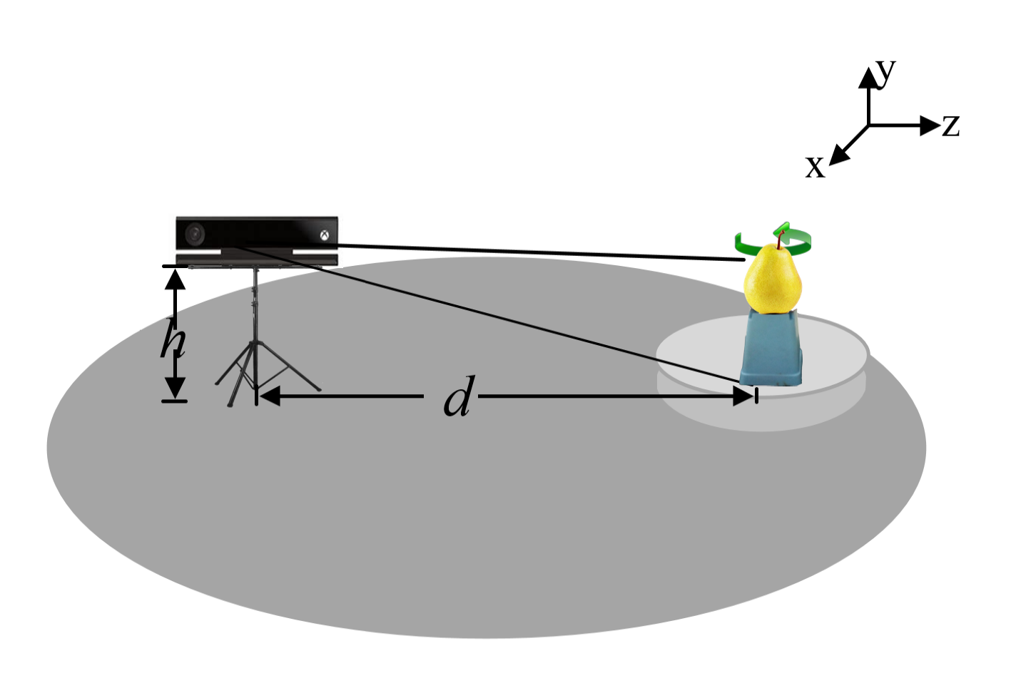
In this experiment, a Kinect v2.0 camera and an electric turntable are used to build a three-dimensional fruit model as shown in Figure 1. During the process of scanning, eight pieces of point clouds (point cloud is collected by rotating every 45°) are registered by the iterative closest point (ICP) algorithm to obtain the initial 360° surface point cloud model. According to the rotation matrix, the subsequent point clouds are rotated around the y-axis in Equation (1). It is specified that the direction parallel to the camera coordinate system is the x-axis, the direction vertical to the camera coordinate system is the y-axis, and the direction parallel between the camera and the object is the z-axis.
where is the point cloud from each direction of the surface, is the processed point cloud by the rotation matrix, and . Based on the first point cloud , rotate the other 7 pieces of point clouds by 45°, 90°, 135°, 180°, 225°, 270°, 315°, and the value of is the angle of rotation.
The basic principle of the ICP [47] algorithm is: Match the target point cloud from one single direction point cloud P to the source point cloud from the adjacent point cloud Q, find the nearest neighbor point according to certain constraints, and then calculate the optimal matching parameters R and t to minimize the error function in Equation (2),
The traditional ICP algorithm can be summarized in two steps: compute correspondences between the two-point cloud; calculate the transformation that minimizes the distance between the corresponding points. For the original point cloud of the model, preprocessing is needed, and the outlier points are removed by the statistic outlier filter [48]. In the process of statistics, the number n of the nearest neighbor point is considered, and the distance from the point to all neighboring points p is calculated to determine whether it is less than the threshold standard deviation of outliers. The point whose average distance is outside the standard range will be removed from the data set. After ICP registration, there are overlapped data in the adjacent patches point cloud, so the normal estimation method based on moving least square (MLS) method is used to resample the point cloud.
2.1. Registration the Surface and Bottom Point Cloud of Fruit Model
When the fruit is placed vertically on the turntable, it cannot photograph the bottom point cloud of the fruit in the experiment. The shape of the fruit bottom is different, there are convex ones, such as eggplant and potato, and concave ones, such as tomato and apple. The bottom is a part of the fruit which will affect the accuracy of the result of measuring, so it is necessary to supplement the points from the bottom.
Because the bottom point cloud is collected in the positive direction of the camera, which is different from the coordinate system of the surface point cloud. The collected bottom point cloud should be rotated 90° around the x-axis so that the bottom and the surface point cloud are in the same coordinate system. Equation (3) shows the bottom point cloud in the same coordinate system as the surface point cloud after rotating along the x-axis. Then, move the centroid of the bottom point cloud to the centroid c of the surface point cloud. It shows that the bottom point cloud is in the same coordinate system as the surface point cloud after moving the centroid to c. Through the rotation matrix and translation vector, the bottom point cloud is processed preliminarily. The initial processed point cloud and the surface point cloud are in the same coordinate system. They are all measured with x-axis as the fruit’s length, y-axis as the height, and z-axis as the width.
where is the initial bottom point cloud, is the bottom point cloud after preliminary matrix operations, is 90°, it means that the angle of bottom point cloud around the x-axis, and is the preliminary translation vector. is in the same coordinate system as the surface point cloud, and the direction of the fruit’s bottom point cloud is downward.
ICP algorithm is still needed to accurately register surface point cloud and bottom point cloud. The rotation matrix and translation vector are obtained by the ICP method below 30 mm of the surface point cloud registering with the processed bottom point cloud. The obtained transformation matrix is also applicable to the whole surface point cloud. Then the whole point cloud is obtained after the surface point cloud and the bottom point cloud registered by and . As shown in Equation (4), the whole point cloud of fruit is
where is the surface point cloud, is the bottom point cloud, and p is the whole point cloud needed in this experiment. Through coarse and precise registration of the surface and bottom points of the point cloud, the whole point cloud is finally obtained.
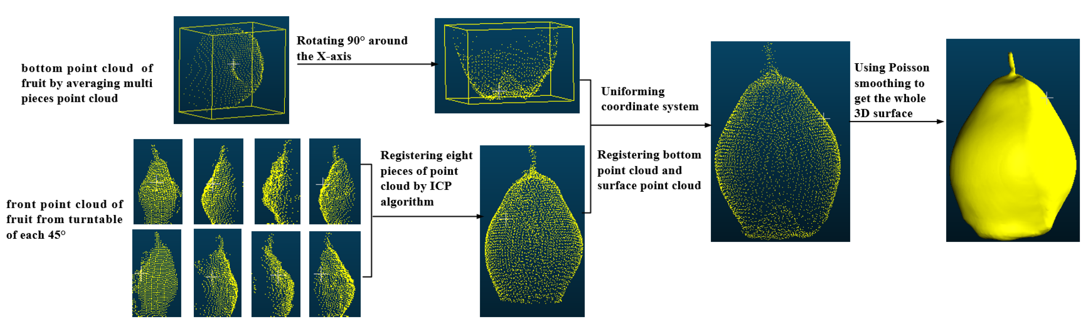
In Figure 2, eight pieces of continuous point clouds are registered together to obtain a complete 360° frontal model, which contains the surface information of the fruit. At this point, the point cloud of the fruit bottom and the point cloud of the front are respectively obtained, and through preliminary processing, they are in the same world coordinate system, because the fruit surface is the convex body, the surface image and the bottom image taken by the camera can simultaneously acquire the characteristics of the points under the side. Then, through the registration of points collected at the bottom side of the fruit in different coordinate systems, the bottom rotation matrix and the translation vector are obtained, and the bottom model is further processed. Through these steps, a point cloud model with shape-preserving, accurate normal, and small curvature variance is obtained. Finally, the whole fruit model is obtained by the Poisson surface reconstruction method for the preprocessing-smoothed model point cloud p. The fruit’s stalk and pulp point cloud is obtained by frontal surface registering, while the fruit’s bottom point cloud is obtained by image acquisition and coordinate system transformation. The pulp and the bottom of the fruit are combination called fruit pulp in the next subsequent chapters, which is convenient for the subsequent separation of the fruit stalk.
2.2. Segmentation the Fruit Stalk
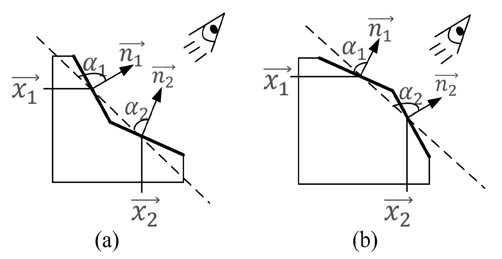
Based on the 3D model, the stalk cannot be counted as the height of the fruit, so the length of the fruit stalk needs to be removed when calculating the height. In this experiment, the stemmed fruits need further treatment for removing stalks by the locally convex connected patches (LCCP) method [49], which does not depend on the color or texture of point cloud, but on the spatial information and normal vector information. For the segmented model, it is necessary to calculate the convexity-concavity relationship of adjacent patches. The relationship is judged by the extended connectivity criterion and sanity criterion. Extended connectivity criterion uses the angle between the centerline vector , and the normal vector , of the adjacent two pieces to judge concavity or convexity. If > , the relationship of the two patch , is concave, otherwise is convex as shown in Figure 3.
Here, is the difference between the vector and , is the cross product between the vector and as shown in Equation (5),
If the relationship between the two pieces is convex, it should be further judged by the sanity criterion. When the angle between and is greater than the threshold , it can be sure that they are convex relations [49] as in Equation (6),
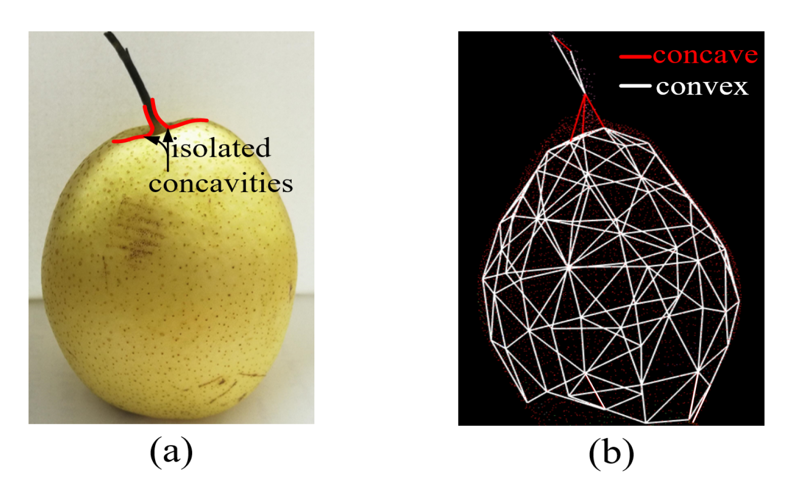
After marking the concavity–convexity relationship of each small region, the region growth algorithm is used to cluster the small region into larger objects. This algorithm restricted by this relationship of small regions can clearly distinguish the boundary between stalk and pulp as shown in Figure 4; the red line represents concavity and the white line represents convexity between adjacent patches. There is an obvious concavity and convexity change at the junction of the fruit’s stalk and pulp, which meets the criteria of LCCP segmentation.
The LCCP algorithm can correctly separate fruit stalk and pulp, which is useful to calculate the actual height of the fruit without stalk using the bounding box method. The point cloud is automatically segmented by convexity–concavity relationship between pulp and stalk, and the compared models are shown in Figure 5. At present, the point cloud is divided into two parts, namely and . The pulp model is retained as the base model for the following measurements.
3. Morphology Measurement of Fruit
3.1. Measurement Length, Height, Width through Principal Component Analysis Bounding-Box Algorithm
When the three-dimensional model is obtained, the length, height, and width of the fruit are calculated first. The steps are as follows: calculating the central point of fruit, where the world coordinate system is the principal direction of point cloud; using the principal direction and centroid establishing the bounding box of the point cloud. As the direction corresponding to the natural axis of the object, the maximum and minimum positions along the three directions of x, y, and z from the vertex are calculated in Equation (7).
By comparing all points , the minimum coordinate point x, the maximum x, the minimum y, the maximum y, the minimum z, and the maximum z have been obtained. Then, combine the minimum values as the minimum point and the maximum value as the maximum point . So, the minimum three-dimensional point and the maximum three-dimensional point in the three-dimensional coordinate system of fruit can be obtained. The center point is the midpoint of the two extreme points, representing the centroid of the bounding box, the center point’s three-dimensional coordinates is shown in Equation (8).
According to the matrix coordinate position of the bounding-box extracted the region of fruit. The effective region includes x, y, and z of fruit, which represent the direction of length, height, and width of fruit respectively. Take the minimum point as the starting point, and the maximum point as the end-point and draw a line from left to right along the main direction x, draw a line from up to down along the main direction y, draw a line from front to back along the main direction z, which represents the length, height, and width of the fruit, respectively. The length of fruit can be obtained by subtracting the left and right limit values of x intersection points, the height can be obtained by subtracting the limit values of y intersection points, and the width can be obtained by subtracting the limit values of z intersection points. The length l, height h, and width w of the bounding box can be obtained by the differences of the three directions of the maximum three-dimensional point and the minimum three-dimensional point in Equation (9).
Based on the bounding-box method, the three-dimensional fruit plane is displayed in Figure 6. It is specified that the x-axis corresponds to the length l and height h of fruit, the y-axis corresponds to the width w and height h of fruit, and the z-axis corresponds to the width w and length l of fruit. The display of the z-direction surface is divided into top and bottom surfaces to observe the top and bottom details.
3.2. Measurement Perimeters of Fruit
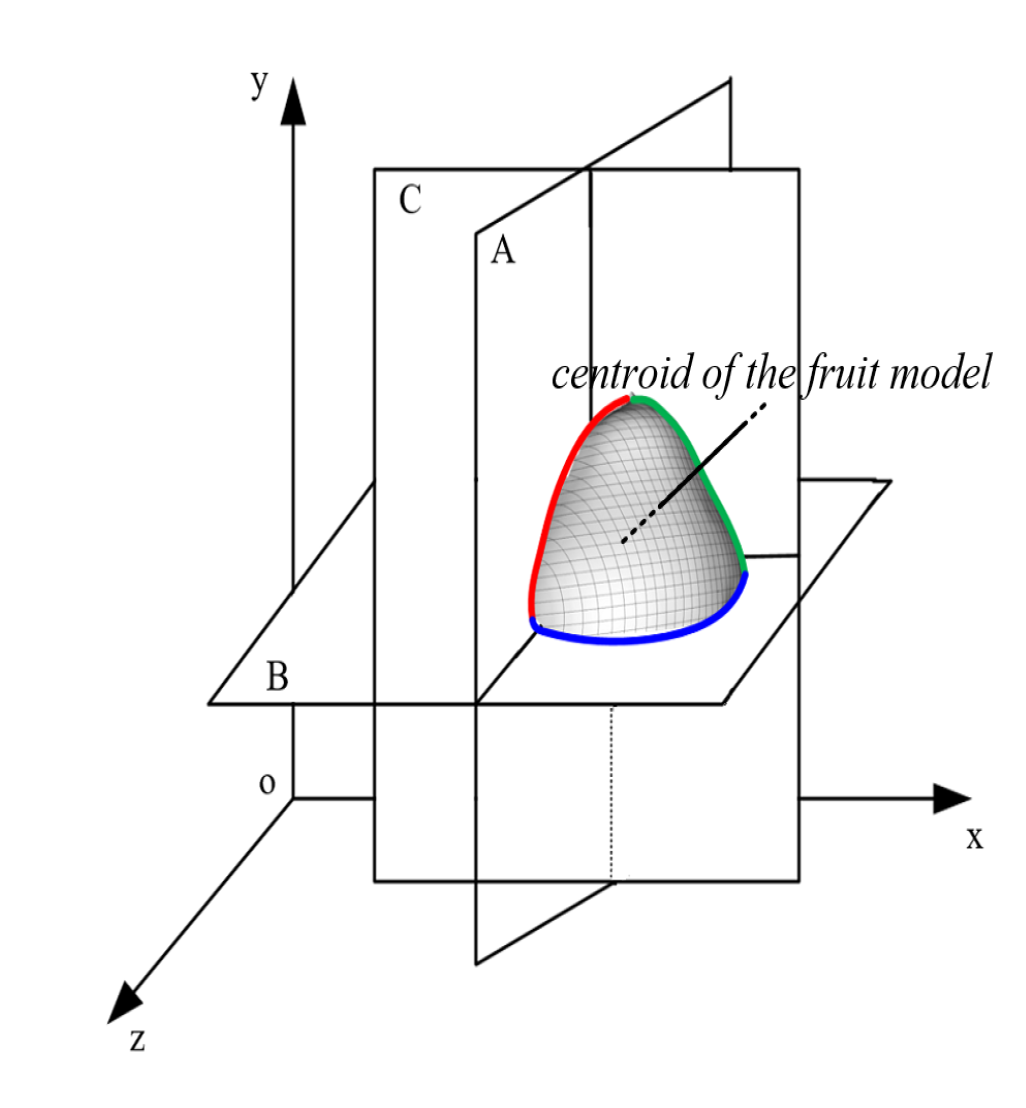
Further, analyzing the contour of the model, and taking the centroid of the model as the research object to calculate the perimeter of each section is another task for fruit. The distribution of three-dimensional continuous image on any plane is called the section of f along plane P. The outline of multi-layer slices can be represented in three-dimensional coordinates. In this experiment, the segmentation point is obtained according to the symmetry of the fruit. The tangent planes are made parallel to , , and , respectively according to the , where section A, B, and C are parallel to plane , plane , and plane , respectively, the points made up of these planes are shown in Equation (10),
Based on the three sections parallel to -axis through the centroid, the intersection point of the fruit model is the set of the required point cloud, which constitutes the contour of the fruit, i.e., the perimeter. The perimeter is of great significance to identify the shape of the fruit. As shown in Figure 7, the contour obtained by plane A tangent to the model is shown in red, the contour obtained by plane B tangent to the model is shown in blue, and the contour obtained by plane C tangent to the model is shown in green. Each plane centered on the intersection is divided into four quadrants, and the intersection of these lines in the two-dimensional plane represents the outline of the fruit.
These points are discrete in two-dimensional space, so the spline interpolation method is used to connect them together. As the surface of the fruit tends to be a sphere or ellipsoid, the obtained points are improved by the cubic Bezier curve spline [50] in Equation (11),
where is the boundary points of the contour, t is the scale value, the smooth curve is drawn according to the coordinates of four adjacent points. Here, we use the method in [51], which not only retains the characteristics of the cubic Bezier curve but also passes through all the points in the experiment, that is, the control point , can be expressed by unit vector and tension parameter. For the continuous curve L on the section, its density distribution function is . Because the function is a piecewise curve, the perimeter is obtained by the curve integral in Equation (12) on each small curve [a, b].
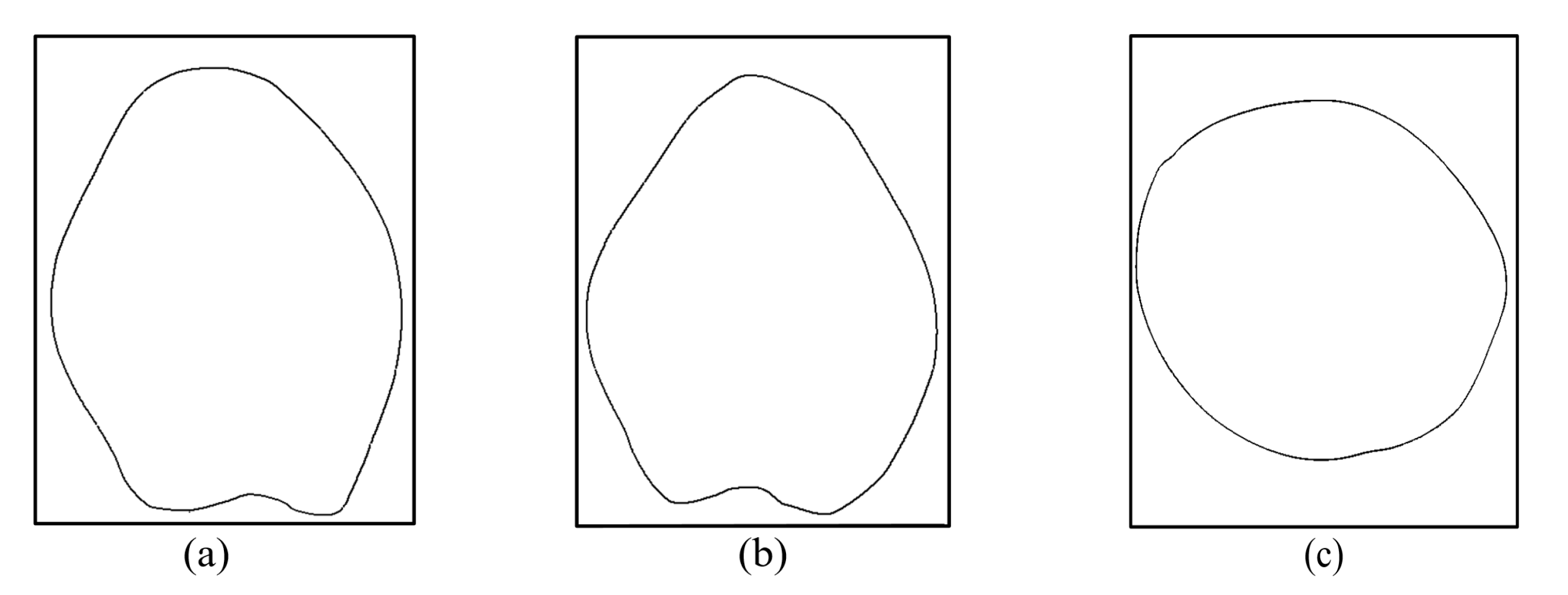
The surface profile is obtained by the intersection of the tangent plane and the parallel section as shown in Figure 8, which are described as the value points of the contour line.
4. Experiment
Two groups of fruits were tested in this paper. In the first group, the predicted value is compared with the measured value after modeling the same type of fruits (pears in this experiment) in different sizes; in the second group, the predicted value is compared with the measured value after modeling many types of fruits with different shapes, colors, textures, and stalks. When practically measured, for the length, width, and height of the fruit, the actual value measured by the ruler is compared with the predicted value; for the perimeter of the fruit, the average value obtained by the soft ruler within 3 mm of the centroid is compared with the predicted value.
4.1. Measurement of the Morphological Parameters of the Pear
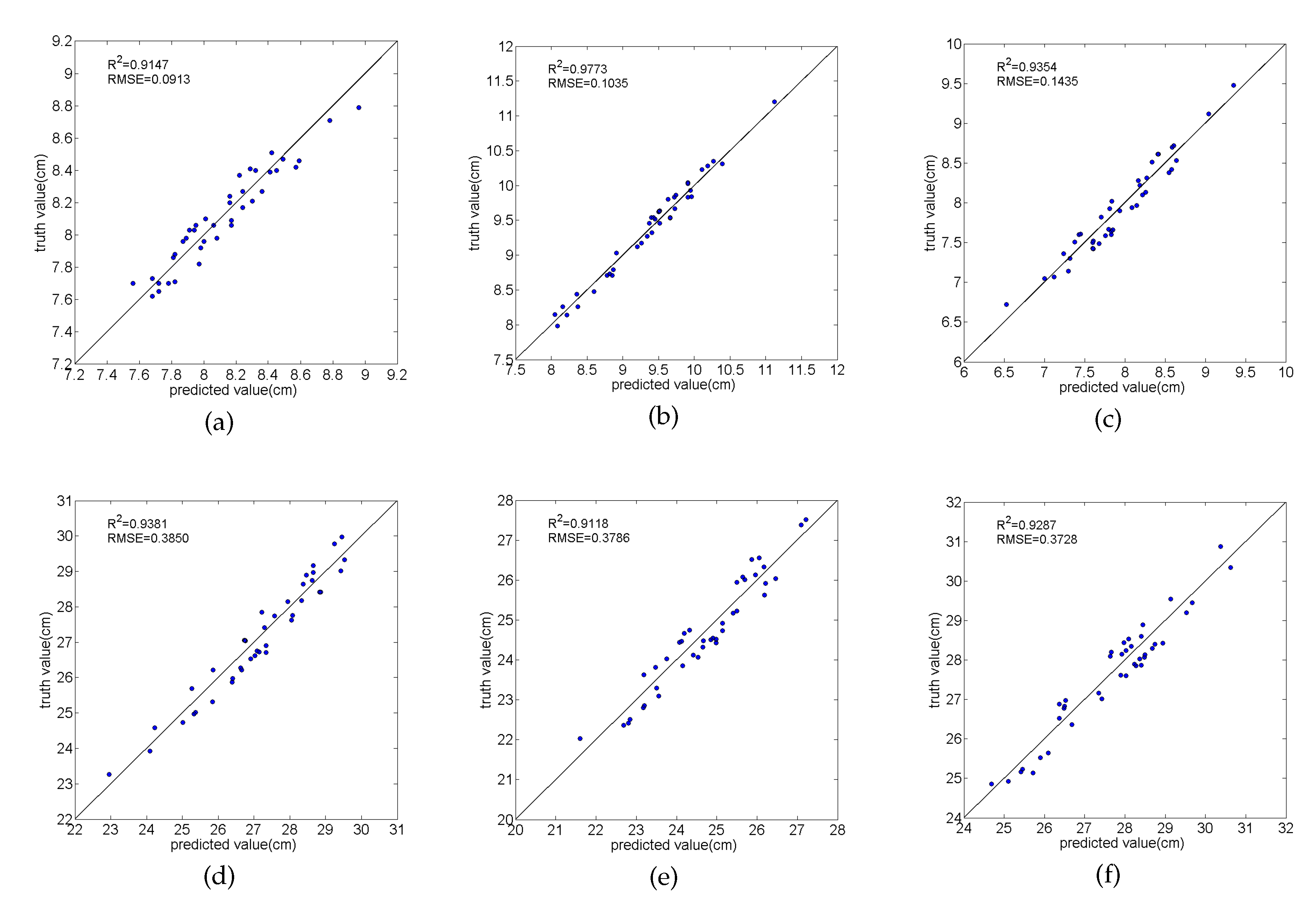
Forty pears are used as experimental objects to verify the validity of the experiment by modeling, measuring and comparing with the actual value. The measured results are compared with predicted values of length, height, width, and perimeter to get the minimum error, maximum error, coefficient of determination (), and root mean square error (). The results are shown in Figure 9. In the coordinate graph, the x-axis represents the predicted value, and the y-axis represents the measured value of pears.
The other methods [5,18,52] are compared with the algorithm proposed in this paper, and the results are shown in Table 1. The value obtained by averaging the length and width is taken as vertical diameters. The results show that average of vertical pear diameter is 1.17 mm and the is 92.5%; the horizontal pear diameter is 1.03 mm and the is 97.7%; the perimeters of the pears are calculated, the smallest error is from the pears’ z-axis perimeters, is 3.72 mm; the largest error is the pears’ x-axis perimeters, is 3.85 mm.
4.2. Measurements of the Morphological Parameters of Many Kinds of Fruit
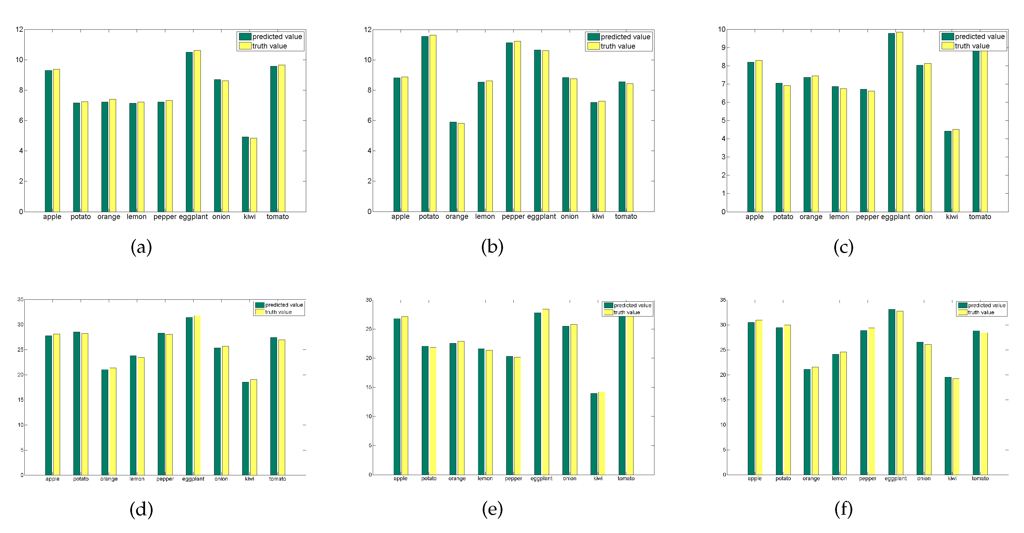
A variety of vegetables and fruits are used as experimental objects to establish a three-dimensional model and calculate the morphological parameters. For onion, pear, kiwifruit, and other fruits with stalks, the LCCP algorithm is used to remove its stalk and calculate the height of the pulp. For fruits without a stalk, like tomato, orange, eggplant, the model calculates the height directly. The measured values and predicted values are shown in Figure 10, the yellow bar represents the predicted value, the green bar represents the measured value. Among various fruit models, the error between the measured value and the predicted value of the green pepper model is larger than other fruits. The shape of the green pepper model is irregular, some details are removed during the point cloud registration process, so the model error of the green pepper is larger than that of other fruits. The details of the model still need to be further studied, which is also the focus of the next work.
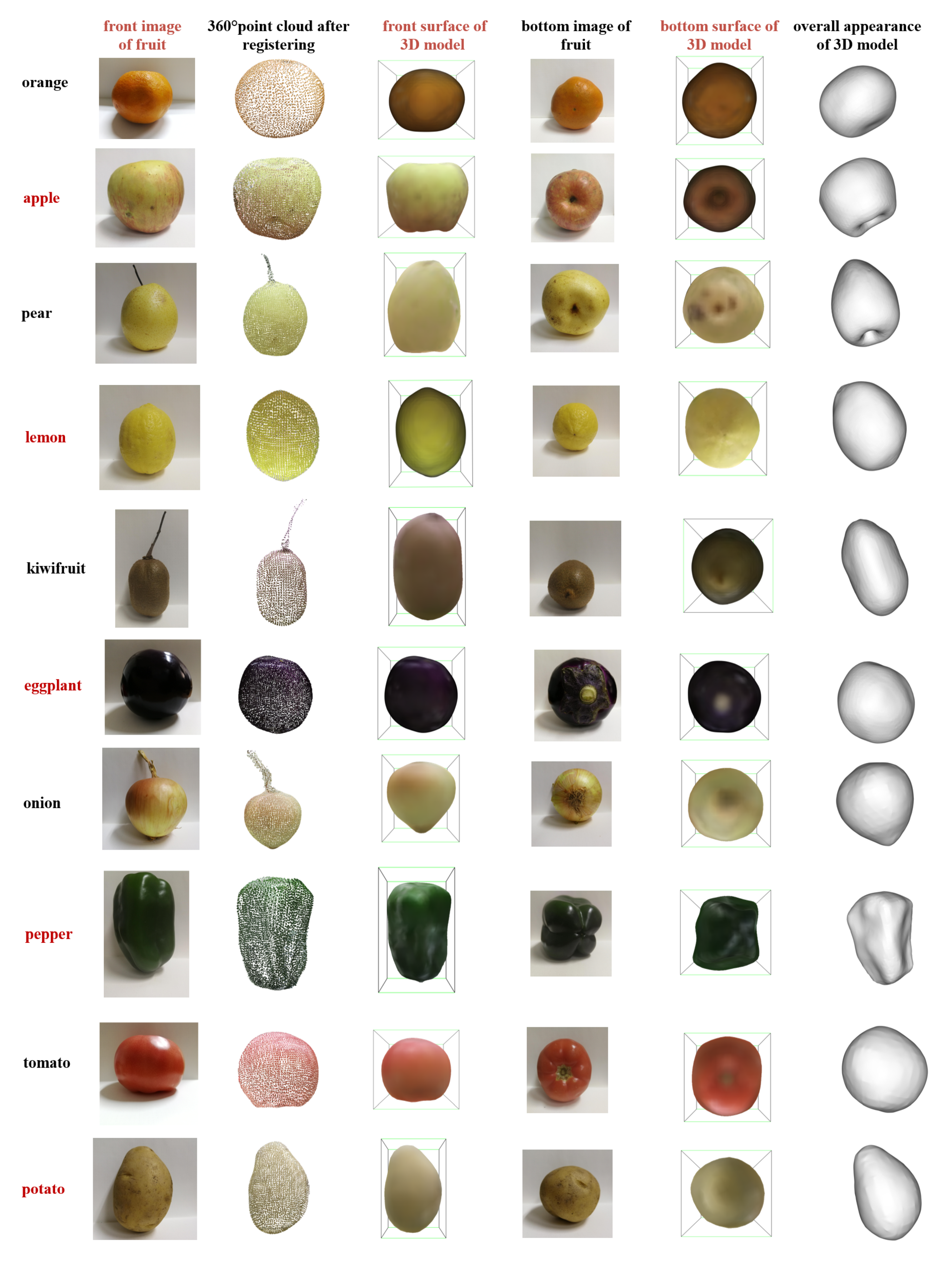
To show the model more clearly, when collecting the point cloud, the Kinect camera coordinate system is used to calibrate the color and depth images, so the collected point cloud has the attributes of color and coordinate position. The fruit model is displayed from the front, bottom, and side, respectively, in the experiment. In Figure A1, from left to right is the front image of fruit, the registering model of the fruit point cloud, the front of 3D model, the bottom image of fruit, the bottom of the 3D model, and the overall appearance of the 3D model. Through the observation of the model by the bounding-box method, it can be seen that the method provided in this experiment can correctly fit the 3D model of fruit. It can not only measure the morphological parameters, such as length, height, width, perimeter but also reflect the color and texture characteristics.
5. Conclusions
The three-dimensional fruit model is obtained by point cloud modeling from different coordinate systems. Eight surface point clouds are registered by the ICP algorithm, the bottom point cloud coordinate system and the surface point cloud coordinate system are unified to get the whole point cloud of the fruit. The fruit model is classified according to its stalk, the height of the fruit without stalk is calculated directly, while the height of fruit with stalk is calculated after further processing. The parameters of length, height, width, and centroid are obtained by the bounding-box method. Through the tangent planes to the fruit model of the centroid and main direction x, y, and z, the contours of the fruit is obtained.
The innovation of this experiment is to obtain a complete model, not just a front surface model of the fruit. Secondly, for the measurement of fruit with stalk, the concavity–convexity relationship between adjacent patches is used as the segmentation judgment standard to remove the fruit stalk to improve the accuracy of height measurement. Finally, the effectiveness of the algorithm is verified by comparing the measured values of the length of the bounding box method and the perimeter of the fruit with the actual values.
In this paper, the length, height, width and three-dimensional perimeters of the fruit are measured and compared with the actual values. In the first group of the experiment, pears with stalks are taken as the research subjects, the concavity and convexity of the LCCP method are used to remove the stalk, then the phenotype parameters of the model are calculated. In the second group, a variety of fruits are taken as the research objects, and the phenotype parameters of fruits with different shapes, color, and texture are measured by our method.
Through the experimental results, it can be seen that the experimental method in this paper is universal and can complete the phenotype parameters measurement of many kinds of fruits.
Author Contributions
Conceptualization, Y.W. and Y.C.; data curation, Y.W. and Y.C.; formal analysis, Y.C.; funding acquisition, Y.C.; investigation, Y.W. and Y.C.; methodology, Y.W.; project administration, Y.C.; resources, Y.C.; software, Y.W. and Y.C.; supervision, Y.C.; validation, Y.W.; visualization, Y.W.; writing—original draft preparation, Y.W. and Y.C.; writing—review and editing, Y.W. and Y.C. All authors have read and agreed to the published version of the manuscript.
Funding
This project is supported by the national key science and technology infrastructure project, “National Research Facility for Phenotypic and Genotypic Analysis of Model Animals”, grant number ”4444-10099609”.
Conflicts of Interest
The authors also thank the editor and anonymous reviewers for providing helpful suggestions for improving the quality of this manuscript.
Abbreviations
The following abbreviations are used in this manuscript:
| 3D | Three-dimensional |
| 2.5D | 2.5-dimensional |
| RGB-D | Red, Green, Blue, and Depth |
| TOF | Time of Flight |
| ROI | Region of Interest |
| v2.0 | Version 2.0 |
| ICP | Iterative Closest Point |
| LCCP | Locally Convex Connected Patches |
| min | Minimum |
| max | Maximum |
Appendix A
Figure A1.
Description of many kinds of fruit models with real images from different directions.

References
- Vázquez-Arellano, M.; Griepentrog, H.W.; Reiser, D.; Paraforos, D.S. 3-D Imaging Systems for Agricultural Applications—A Review. Sensors 2016, 16, 618. [Google Scholar] [CrossRef] [Green Version]
- Bhargava, A.; Bansal, A. Fruits and vegetables quality evaluation using computer vision: A review. J. King Saud Univ. Comput. Inf. Sci. 2018. [Google Scholar] [CrossRef]
- Rashidi, M.; Gholami, M.; Abbassi, S. Cantaloupe Volume Determination through Image Processing. J. Agric. Sci. Technol. 2009, 11, 623–631. [Google Scholar]
- Su, Q.; Kondo, N.; Li, M.; Sun, H.; AI Riza, D.F. Potato feature prediction based on machine vision and 3D model rebuilding. Comput. Electron. Agric. 2017, 137, 41–51. [Google Scholar] [CrossRef]
- Wang, W.; Li, C. Size estimation of sweet onions using consumer-grade RGB-depth sensor. J. Food Eng. 2014, 142, 153–162. [Google Scholar] [CrossRef]
- Lu, Y.; Lu, R. Phase analysis for three-dimensional surface reconstruction of apples using structured-illumination reflectance imaging. In Proceedings of the Sensing for Agriculture and Food Quality and Safety IX. International Society for Optics and Photonics, Anaheim, CA, USA, 9–13 April 2017. [Google Scholar]
- Fukui, R.; Schneider, J.; Nishioka, T.; Warisawa, S.; Yamada, I. Growth Measurement of Tomato Fruit based on Whole Image Processing. In Proceedings of the 2017 IEEE International Conference on Robotics and Automation (ICRA), Singapore, 29 May–3 June 2017. [Google Scholar]
- Zhu, B. Three-dimensional shape enhanced transform for automatic apple stem-end/calyx identification. Opt. Eng. 2007, 46, 017201. [Google Scholar]
- He, J.Q.; Harrison, R.J.; Li, B. A novel 3D imaging system for strawberry phenotyping. Plant Methods 2017, 13, 93. [Google Scholar] [CrossRef]
- Zhang, Y.; Teng, P.; Shimizu, Y.; Hosoi, F.; Omasa, K. Estimating 3D Leaf and Stem Shape of Nursery Paprika Plants by a Novel Multi-Camera Photography System. Sensors 2016, 16, 874. [Google Scholar] [CrossRef] [Green Version]
- Ivanov, A.G.; Huner, N.P.; Grodzinski, B.; Patel, R.V.; Barron, J.L. Computer Vision Based Autonomous Robotic System for 3D Plant Growth Measurement. In Proceedings of the Canadian Conference on Computer and Robot Vision, Halifax, NS, Canada, 3–5 June 2015; pp. 290–296. [Google Scholar]
- Kochi, N.; Tanabata, T.; Hayashi, A.; Isobe, S. A 3D Shape-Measuring System for Assessing Strawberry Fruits. Int. J. Autom. Technol. 2018, 12, 395–404. [Google Scholar] [CrossRef]
- Gaspar, M.; Pascoalfaria, P.; Amado, S.; Alves, N. A Computer Tool for 3D Shape Recovery of Fruits. In Applied Mechanics and Materials; Trans Tech Publications: Zürich, Switzerland, 2019; pp. 181–189. [Google Scholar]
- Kabutey, A.; Hrabe, P.; Mizera, C.; Herak, D. 3D image analysis of the shapes and dimensions of several tropical fruits. Agron. Res. 2018, 1383–1387. [Google Scholar]
- Gongal, A.; Karkee, M.; Amatya, S. Apple fruit size estimation using a 3D machine vision system. Inf. Process. Agric. 2018, 5, 498–503. [Google Scholar] [CrossRef]
- Golbach, F.; Kootstra, G.; Damjanovic, S.; Otten, G.; Zedde, R.V.D. Validation of plant part measurements using a 3D reconstruction method suitable for high-throughput seedling phenotyping. Mach. Vis. Appl. 2016, 27, 663–680. [Google Scholar] [CrossRef] [Green Version]
- Whan, A.; Smith, A.B.; Cavanagh, C.; Ral, J.; Shaw, L.M.; Howitt, C.A.; Bischof, L. GrainScan: A low cost, fast method for grain size and colour measurements. Plant Methods 2014, 10, 23. [Google Scholar] [CrossRef] [Green Version]
- Yamamoto, S.; Karkee, M.; Kobayashi, Y.; Nakayama, N.; Tsubota, S.; Thanh, L.N.; Konya, T. 3D reconstruction of apple fruits using consumer-grade RGB-depth sensor. Eng. Agric. Environ. Food 2018, 11, 159–168. [Google Scholar] [CrossRef]
- Li, X.F.; Zhu, W.X.; Hua, X.P.; Kong, L.D. Apple grading detection based on fusion of shape and color features. Comput. Eng. Appl. 2010, 46, 206–208. [Google Scholar]
- Arakeri, M.P. Computer Vision Based Fruit Grading System for Quality Evaluation of Tomato in Agriculture industry. Procedia Comput. Sci. 2016, 79, 426–433. [Google Scholar] [CrossRef] [Green Version]
- Fu, L.; Sun, S.; Li, R.; Wang, S. Classification of Kiwifruit Grades Based on Fruit Shape Using a Single Camera. Sensors 2016, 16, 1012–1026. [Google Scholar] [CrossRef] [Green Version]
- Wang, H.; Xiong, J.; Li, Z.; Deng, J.; Zou, X. Potato grading method of weight and shape based on imaging characteristics parameters in machine vision system. Trans. Chin. Soc. Agric. Eng. 2016, 32, 272–277. [Google Scholar]
- Sofu, M.M.; Er, O.; Kayacan, M.C.; Cetisli, B. Design of an automatic apple sorting system using machine vision. Comput. Electron. Agric. 2016, 127, 395–405. [Google Scholar] [CrossRef]
- Vitzrabin, E.; Edan, Y. Adaptive thresholding with fusion using a RGBD sensor for red sweet-pepper detection. Biosyst. Eng. 2016, 146, 45–56. [Google Scholar] [CrossRef]
- Tushar, J.; Kulbir, S.; Aditya, A. Volumetric estimation using 3D reconstruction method for grading of fruits. Multimed. Tools Appl. 2019, 78, 1613–1634. [Google Scholar]
- Priti, S.; Nidhi, G. Auto-annotation of tomato images based on ripeness and firmness classification for multimodal retrieval. In Proceedings of the ICACCI 2016, Jaipur, India, 21–24 September 2016. [Google Scholar]
- Hu, Z.; Tang, J.; Zhang, P. Fruit bruise detection based on 3D meshes and machine learning technologies. In Proceedings of the Mobile Multimedia/Image Processing, Security, & Applications. International Society for Optics and Photonics, Baltimore, MD, USA, 17–21 April 2016. [Google Scholar]
- Qureshi, W.S.; Payne, A.; Walsh, K.B.; Linker, R.; Cohen, O.; Dailey, M.N. Machine vision for counting fruit on mango tree canopies. Precis. Agric. 2017, 18, 224–244. [Google Scholar] [CrossRef]
- Wang, Z.; Walsh, K.B.; Verma, B. On-Tree Mango Fruit Size Estimation Using RGB-D Images. Sensors 2017, 17, 2738. [Google Scholar] [CrossRef] [Green Version]
- Stein, M.; Bargoti, S.; Underwood, J. Image Based Mango Fruit Detection, Localisation and Yield Estimation Using Multiple View Geometry. Sensors 2016, 16, 1915. [Google Scholar] [CrossRef]
- Gongal, A.; Amatya, S.; Karkee, M.; Zhang, Q.; Lewis, K. Sensors and systems for fruit detection and localization. Comput. Electron. Agric. 2015, 116, 8–19. [Google Scholar] [CrossRef]
- Min, R.; Kose, N.; Dugelay, J.L. KinectFaceDB: A Kinect Database for Face Recognition. IEEE Trans. Syst. Man Cybern. Syst. 2014, 44, 1534–1548. [Google Scholar] [CrossRef]
- Li, B.Y.L.; Mian, A.S.; Liu, W.; Krishna, A. Using Kinect for face recognition under varying poses, expressions, illumination and disguise. In Proceedings of the 2013 IEEE Workshop on Applications of Computer Vision (WACV), Tampa, FL, USA, 15–17 January 2013. [Google Scholar]
- Hg, R.I.; Jasek, P.; Rofidal, C.; Nasrollahi, K.; Moeslund, T.B.; Tranchet, G. An RGB-D Database Using Microsoft’s Kinect for Windows for Face Detection. In Proceedings of the International Conference on Signal Image Technology & Internet Based Systems, Naples, Italy, 25–29 November 2012. [Google Scholar]
- Li, B.Y.L.; Mian, A.S.; Liu, W.; Krishna, A. Face recognition based on Kinect. Pattern Anal. Appl. 2016, 19, 977–987. [Google Scholar] [CrossRef]
- Lee, G.C.; Yeh, F.H.; Hsiao, Y.H. Kinect-based Taiwanese sign-language recognition system. Multimed. Tools Appl. 2016, 75, 261–279. [Google Scholar] [CrossRef]
- Giuroiu, M.C.; Marita, T. Gesture recognition toolkit using a Kinect sensor. In Proceedings of the IEEE International Conference on Intelligent Computer Communication & Processing, Cluj-Napoca, Romania, 3–5 September 2015. [Google Scholar]
- Siddiqui, S.A.; YusraSnober Raza, S.; Khan, F.M.; Syed, T.Q. Arm Gesture Recognition on Microsoft Kinect Using a Hidden Markov Model- based Representation of Poses. In Proceedings of the International Conference on Information and Communication Technologies, Karachi, Pakistan, 12–13 December 2015. [Google Scholar]
- Li, H.; Yang, L.; Wu, X.; Xu, S.; Wang, Y. Static Hand Gesture Recognition Based on HOG with Kinect. In Proceedings of the International Conference on Intelligent Human-machine Systems & Cybernetics, Nanchang, China, 26–27 August 2012. [Google Scholar]
- Deng, R.; Zhou, L.L.; Ying, R.D. Gesture extraction and recognition research based on Kinect depth data. Appl. Res. Comput. 2013, 30, 1262–1263. [Google Scholar]
- Fan, Z.; Xu, J.; Liu, W.; Liu, F.; Cheng, W. Kinect-based dynamic head pose recognition in online courses. In Proceedings of the 2016 IEEE Advanced Information Management, Communicates, Electronic and Automation Control Conference (IMCEC), Xi’an, China, 3–5 October 2016. [Google Scholar]
- Anwar, S.; Ayoub, A.H.; Ahmed, G. Head Pose Estimation on Top of Haar-Like Face Detection: A Study Using the Kinect Sensor. Sensors 2015, 15, 20945–20966. [Google Scholar]
- Darby, J.; Sánchez, M.B.; Butler, P.B.; Loram, I.D. An evaluation of 3D head pose estimation using the Microsoft Kinect v2. Gait Posture 2016, 48, 83–88. [Google Scholar] [CrossRef] [PubMed] [Green Version]
- Le, T.L.; Nguyen, M.Q.; Nguyen, T.T.M. Human posture recognition using human skeleton provided by Kinect. In Proceedings of the 2013 International Conference on Computing, Management and Telecommunications (ComManTel), Ho Chi Minh City, Vietnam, 21–24 January 2013. [Google Scholar]
- Kim, D.H.; Kwak, K.C. Classification of K-Pop Dance Movements Based on Skeleton Information Obtained by a Kinect Sensor. Sensors 2017, 17, 1261. [Google Scholar] [CrossRef] [PubMed] [Green Version]
- Andersson, V.; Dutra, R.; Araújo, R. Anthropometric and human gait identification using skeleton data from Kinect sensor. In Proceedings of the 29th Annual ACM Symposium on Applied Computing (SAC), Gyeongju, Korea, 24–28 March 2014. [Google Scholar]
- Besl, P.; McKay, N. A Method for Registration of 3-D Shapes. IEEE Trans. Pattern Anal. Mach. Intell. 1992, 14, 239–256. [Google Scholar] [CrossRef]
- Rusu, R.B.; Marton, Z.C.; Blodow, N.; Dolha, M.E.; Beetz, M. Towards 3D Point cloud based object maps for household environments. Robot. Auton. Syst. 2008, 56, 927–941. [Google Scholar] [CrossRef]
- Stein, S.C.; Schoeler, M.; Papon, J.; Worgotter, F. Object Partitioning Using Local Convexity. In Proceedings of the IEEE Conference on Computer Vision and Pattern Recognition (CVPR), Columbus, OH, USA, 23–28 June 2014. [Google Scholar]
- Hobby, J.D. Smooth, easy to compute interpolating splines. Discret. Comput. Geom. 1986, 1, 123–140. [Google Scholar] [CrossRef]
- Will Robertson MathWorks Community Profile. Available online: https://ww2.mathworks.cn/matlabcentral/profile/authors/3365332-will-robertson (accessed on 21 February 2020).
- Xu, S.; Lu, K.; Pan, L.; Liu, T.; Zhou, Y.; Wang, B. 3D Reconstruction of Rape Branch and Pod Recognition Based on RGB-D Camera. Trans. Chin. Soc. Agric. Mach. 2019, 2, 21–27. [Google Scholar]
Figure 1.
Point cloud acquisition with the Kinect and turntable in the experiment.

Figure 2.
Registering the whole model of fruit using point cloud from different coordinate systems.

Figure 3.
Basic principles of judging concavity and convexity adjacent patches for the locally convex connected patches (LCCP) method. (a) The relationship between the two patches is concave. (b) The relationship between the two patches is convex.
Figure 3.
Basic principles of judging concavity and convexity adjacent patches for the locally convex connected patches (LCCP) method. (a) The relationship between the two patches is concave. (b) The relationship between the two patches is convex.

Figure 4.
Judgment of the relationship between the adjacent patches of fruit stalk and pulp by concavity and convexity method. (a) Judgment of the boundary based on the relationship of the pear’s surface. (b) Concavity–convexity characteristics of each patch on the three-dimensional mesh of the pear surface.

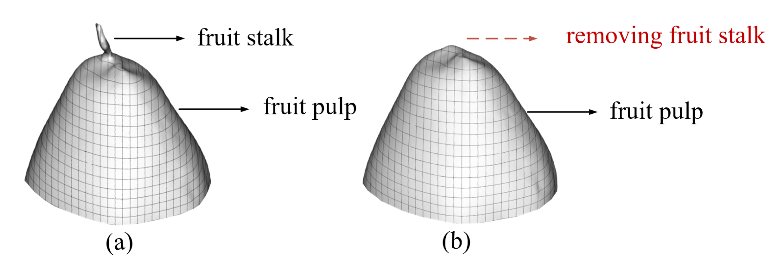
Figure 5.
Comparison of the original pear head model and the segmented model. (a) Top of the original model. (b) Top of the model after segmenting fruit stalk and pulp.
Figure 5.
Comparison of the original pear head model and the segmented model. (a) Top of the original model. (b) Top of the model after segmenting fruit stalk and pulp.

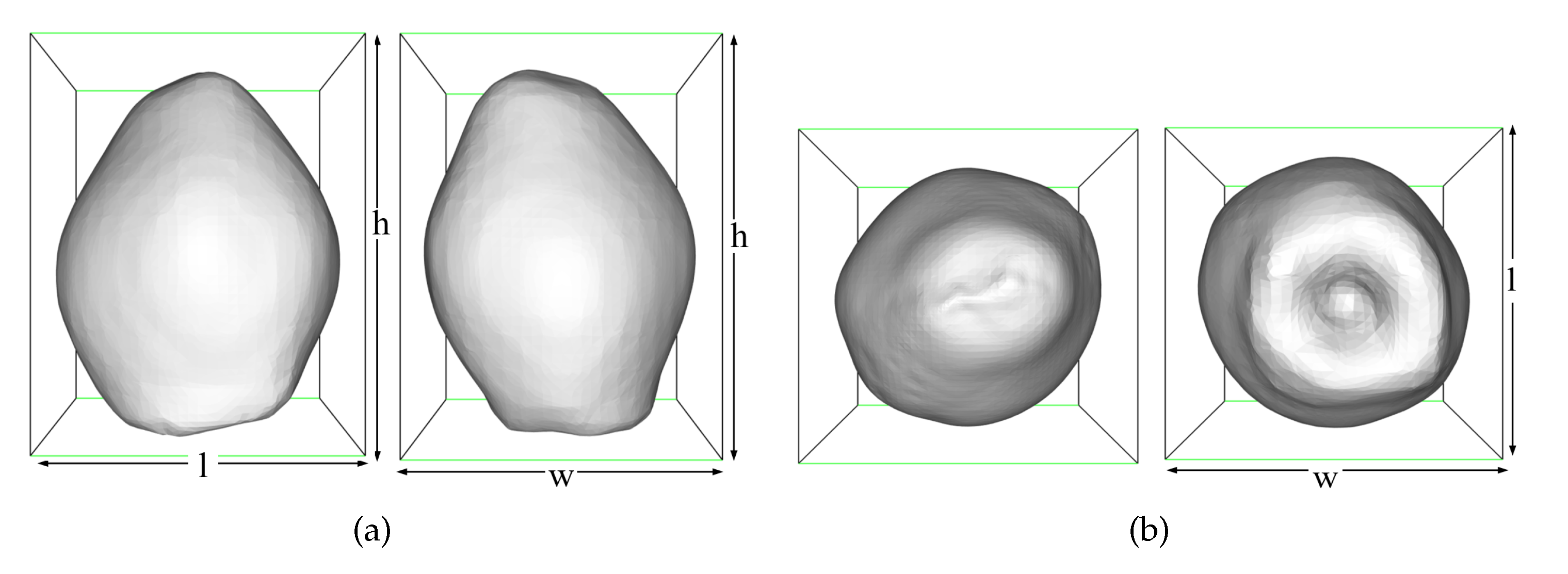
Figure 6.
Measurement length, height, and width of the pear model through the bounding-box algorithm. (a) 3D model of the pear’s front and lateral surface. (b) 3D model of the pear’s top and bottom surface.
Figure 6.
Measurement length, height, and width of the pear model through the bounding-box algorithm. (a) 3D model of the pear’s front and lateral surface. (b) 3D model of the pear’s top and bottom surface.

Figure 7.
Section coordinate system of plane , and C tangent to the fruit model by the centroid.

Figure 8.
Contour obtained by plane and C tangent to the fruit model. (a) Contour obtained by plane A tangent to the fruit model. (b) Contour obtained by plane C tangent to the fruit model. (c) Contour obtained by plane B tangent to the fruit model.
Figure 8.
Contour obtained by plane and C tangent to the fruit model. (a) Contour obtained by plane A tangent to the fruit model. (b) Contour obtained by plane C tangent to the fruit model. (c) Contour obtained by plane B tangent to the fruit model.

Figure 9.
The phenotypes include length, height, width, x-axis perimeter, y-axis perimeter, and z-axis perimeter, recording as (a–f). (a) Comparison of length values. (b) Comparison of height values. (c) Comparison of width values. (d) Comparison of x-axis perimeter. (e) Comparison of y-axis perimeter. (f) Comparison of z-axis perimeter.

Figure 10.
Comparison of predicted and measured values of many kinds of fruit models. The phenotypes include length, height, width, x-axis perimeter, y-axis perimeter, and z-axis perimeter, recording as (a–f). (a) Comparison of length values. (b) Comparison of height values. (c) Comparison of width values. (d) Comparison of x-axis perimeter. (e) Comparison of y-axis perimeter. (f) Comparison of z-axis perimeter.


Table 1.
Comparison of the method in this paper with other methods.
| Experiment | RMSE (mm) | |
|---|---|---|
| Onion maximum diameter [5] | 0.96 | 2.0 |
| Apple largest diameter [18] | 0.968 | 0.8 |
| Rape pod diameter [52] | - | 0.48 |
| Average of vertical pear diameter | 0.925 | 1.17 |
| Average of horizontal pear diameter | 0.977 | 1.03 |
| Pear x-axis perimeters | 0.938 | 3.85 |
| Pear y-axis perimeters | 0.911 | 3.78 |
| Pear z-axis perimeters | 0.928 | 3.72 |
© 2020 by the authors. Licensee MDPI, Basel, Switzerland. This article is an open access article distributed under the terms and conditions of the Creative Commons Attribution (CC BY) license (http://creativecommons.org/licenses/by/4.0/).
Share and Cite
MDPI and ACS Style
Wang, Y.; Chen, Y. Fruit Morphological Measurement Based on Three-Dimensional Reconstruction. Agronomy 2020, 10, 455. https://doi.org/10.3390/agronomy10040455
AMA Style
Wang Y, Chen Y. Fruit Morphological Measurement Based on Three-Dimensional Reconstruction. Agronomy. 2020; 10(4):455. https://doi.org/10.3390/agronomy10040455
Chicago/Turabian StyleWang, Yawei, and Yifei Chen. 2020. "Fruit Morphological Measurement Based on Three-Dimensional Reconstruction" Agronomy 10, no. 4: 455. https://doi.org/10.3390/agronomy10040455
Note that from the first issue of 2016, this journal uses article numbers instead of page numbers. See further details here.