Spatial and Temporal Stability of Weed Patches in Cereal Fields under Direct Drilling and Harrow Tillage

Abstract

The adoption of conservation agriculture (CA) techniques by farmers is changing the dynamics of weed communities in cereal fields and so potentially their spatial distribution. These changes can challenge the use of site-specific weed control, which is based on the accurate location of weed patches for spraying. We studied the effect of two types of CA (direct drilling and harrow-tilled to 20 cm) on weed patches in a three-year survey in four direct-drilled and three harrow-tilled commercial fields in Catalonia (North-eastern Spain). The area of the ground covered by weeds (hereafter called “weed cover”) was estimated at 96 to 122 points measured in each year in each field, in 50 cm × 50 cm quadrats placed in a 10 m × 10 m grid in spring. Bromus diandrus, Lolium rigidum, and Papaver rhoeas were the main weed species. The weed cover and degree of aggregation for all species varied both between and within fields, regardless of the kind of tillage. Under both forms of soil management all three were aggregated in elongated patterns in the direction of traffic. Bromus was generally more aggregated than Lolium, and both were more aggregated than Papaver. Patches were stable over time for only two harrow-tilled fields with Lolium and one direct-drilled field with Bromus, but not in the other fields. Spatial stability of the weeds was more pronounced in the direction of traffic. Herbicide applications, crop rotation, and traffic seem to affect weed populations strongly within fields, regardless of the soil management. We conclude that site-specific herbicides can be applied to control these species because they are aggregated, although the patches would have to be identified afresh in each season.

1. Introduction

Weeds are one of the most significant threats to crop production worldwide. Crop losses in yield and quality due to weeds, as well as costs of control, have a significant economic impact on crop production. In Australia, Llewellyn et al. [1] reported that weeds in their Mediterranean climate area cost Australian grain growers $100/ha in expenditure and losses, with an average expenditure estimated at $75/ha, including herbicide and non-herbicide practices. In Mediterranean rainfed areas of Spain, the reduction of grain crop yield due to competition by the major winter annual grass weeds such as Lolium rigidum, Avena sterilis, and Bromus diandrus and broad-leaved weeds such as Papaver rhoeas is the main concern of the farmers. We know of no data on economic impact of these weeds on the crops of this region, but yield losses in cereals have been quantified to be as large as 85% for severe infestations (1000 plants/m²) of Lolium [2], 50% for infestations of more than 300 panicles/m² of Avena [3] and 71% for severe infestations (500 plants/m²) of Bromus [4]. Papaver has been reported to reduce crop yields between 6% and 70%, depending on crop density, degree of infestation and season [5].

Farmers increasingly wish to control weeds by varying the application of herbicides to match the degree of infestation and positions of the weeds within individual fields [6]. Such site-specific treatments depend on farmers’ knowing where (and when) those weeds are. This knowledge can be obtained in real time from sensors on tractors [7,8], from weed maps created from aerial images taken by unmanned aerial vehicles [9,10] or maps made by interpolation from weed counts in the field and subsequent geostatistical analysis [6,11]. Mapping weed distributions from aerial imagery requires special software, such as that in geographic information systems (GIS) and the purchase of the images, which can be expensive. Mapping from weed surveys has the advantage of more accurate discrimination between weeds and crop plants, and it is better at detecting weeds early in the season when they are sparse. Although this technique seems to be time-consuming and laborious, the economic advantages of using these maps depends on the number of seasons in which a map can accurately depict the same weed patches, i.e., depends on weed patches’ being stable in location [12]. Some species of weeds have been found to remain in place in diverse crops and under various forms of soil management from year to year. Examples include Abutilon theophrasti [13], Solanum nigrum and Chenopodium album [14], Echinochloa crus-galli [15] and Avena sterilis [16]. Other weeds seem to be stable in some situations and not others. These include E. crus-galli [14], Polygonum aviculare and Papaver rhoeas [17]. Detection of stability seems to depend on the density of the populations: the sparser are the weeds, the more difficult it is to detect them [14,17]. Ecological factors such as wind dispersed seeds [14] or post-harvest dispersal [18] may also contribute to the lack of stability over time.

The studies cited above were made in fields where tillage has tended to homogenize the distribution of weed seeds throughout the field [19]. Now, in rainfed Mediterranean agroecosystems, farmers are increasingly adopting conservation agriculture (CA) techniques based on the principles of minimal soil disturbance, permanent soil cover, and crop rotation. Minimal soil disturbance should lead to an increase or maintenance of the soil’s organic matter content and capacity to store water. This can be achieved without inversion of the soil, by harrowing or by direct drilling or no-tillage. Of the two, direct drilling is the most popular, especially where the previous crops have been harvested and the straw removed [20]. But the CA systems, particularly those involving direct drilling, cause changes in the weed communities [21] and a redistribution of the weed flora within the fields, because these practices disperse seeds less [19]. As the seeds of the most important weeds in cereal crops are not airborne, we can expect these species to maintain their locations more in direct drilling systems than under tillage. For those species that remain in place, maps made in one year should be usable in subsequent years for targeted application of herbicide.

Although weed patchiness in CA systems have been studied [22,23], we know of no data on weed patch stability under these systems. We therefore aimed to discover whether soil management (direct drilling versus harrow tillage) influences the spatial distribution of weeds and whether this spatial distribution remains stable over time. Our hypothesis is that direct drilling leads to stronger spatial structure (patchier distribution of weeds) than harrow tillage. To that end, we explored data on the spatial variation of weed cover in several fields. Our aim was to discover what spatial or temporal structures there were in the weed communities and how these might be affected by cultivation. We describe the data with statistical models and quantify both weed aggregation and spatial and temporal variation. If there is a strong spatial aggregation that persists from year to year then a farmer would be able to use maps of weed distribution made in one year for weed control in subsequent years.

2. Materials and Methods

2.1. Field Locations

In 2011, 2012 and 2013 three cereal fields managed with harrowing tillage (T) and four fields managed with by direct drilling (D) in Catalonia (north-eastern Spain) were surveyed for weeds. The tilled fields were at Balaguer (41°46′16″ N–0°45′12″ E), Bellmunt (41°46′34″ N–0°58′35″ E) and Vilanova de Bellpuig (41°35′34″ N–0°58′45″ E). There the soil was tilled by harrow to 20 cm soon after harvest in July and then again shortly before sowing the next crop field in November. The direct-drilled fields were at Agramunt (41°46′10″ N–1°4′42″ E), Bellmunt (41°46′10″ N–1°4′42″ E), Mas de Melons (41°29′14″ N, 0°42′36″ E) and Vilanova de Bellpuig (41°35′17″ N–0°58′37″ E). None of the fields had a notable slope. In these locations the crops were sown without any prior soil cultivation and with minimal soil disruption. In all locations, cereal was sown in November, and sowing rates were in the range 180 to 200 kg ha⁻¹ (

Table 1. Location of the fields, soil management, crops, and herbicide application carried out in each field and year.

Site	Tillage 1	Direction of Traffic	Crop			Herbicide 2
			2011	2012	2013	2011	2012	2013
Agramunt	D (1997)	E–W	Wheat	Barley	Barley	B	B+G	B
Balaguer	T	E–W	Barley	Barley	Barley	B+G 3	B+G	B+G
Bellmunt	T	E–W	Wheat	Wheat	Barley	B+G	B+G	B+G
Bellmunt	D (2007)	N–S	Barley	Barley	Triticale	B+G	B+G	None
Mas de Melons	D (2008)	E–W	Barley	Fallow	Barley	B+G	None	B+G
Vilanova	T	N–S	Barley	Barley	Barley	B+G	B+G	G
Vilanova	D (2002)	N–S	Oat	Barley	Oat	None	B	None

¹ D: direct drill (year of); T: Harrow tillage with a disc harrow at 20 cm deep before sowing. ² B: Broad-leaved herbicide; G: Grass–weed herbicide. ³ Serious concerns about weed resistance to the herbicides applied.

). All fields were farmed on a commercial basis and followed varied crop rotations. Post-emergence herbicides against broad-leaved and grass weeds were applied in most fields although not every year (Table 1). Some herbicides did not target the species that we studied, particularly when only broad-leaved herbicide was applied, but grasses were present (direct drilling fields of Agramunt 2011 and 2013 and Vilanova 2012). All the crops were harvested in June by combine harvester, and the straw removed from the field. In each field, all the traffic for cultivation, sowing, and harvesting was in the same direction. Temperature and rainfall data during the growing seasons were obtained from the meteorological station nearest to each field.

2.2. Sampling

Sampling was carried out each year before herbicide treatments. Weeds were recorded at the same points by estimation of weed cover (percentage of ground covered by weeds) for each species in 50 cm × 50 cm quadrats located at the nodes of a 10 m × 10 m grid. As our study was aimed to provide information to farmers for their management the grid-scale was set to 10 m because this distance is typical of the width of sprayer booms used in the region, even though weed patches smaller than 10 m could be missed. Each grid node was georeferenced with a GPS (Leica CS10, Leica Geosystems AG, St. Gallen, Switzerland) to the nearest centimeter so that weed cover could be observed and recorded in the same place each year. The number of grid nodes varied according to the shapes and sizes of the fields. All the surveys were made during February to May (see

Table 2. Main weed species of each field, sampling area, and date and crop development at the time of sampling.

Field 1	Species	Field Size m × m	Sampling Date			Crop Height cm			Crop Growth Stage 2
			2011	2012	2013	2011	2012	2013	2011	2012	2013
Agramunt-D	Bromus diandrus	50 × 150	18/04	15/02	02/05	60	15	75	55	23	65
Balaguer-T	Lolium rigidum Papaver rhoeas	60 × 100	15/04	26/04	13/05	25	65	45	31	55	33
Bellmunt-T	Lolium rigidum	50 × 150	04/05	15/02	13/05	75	15	65	55	33	55
Bellmunt-D	Bromus diandrus	150 × 50	04/05	15/02	13/05	80	15	100	55	33	55
Mas de Melons-D	Lolium rigidum	100 × 100	12/04	14/02	13/05	30	-- 3	45	33	-- 3	33
	Papaver rhoeas
Vilanova-T	Lolium rigidum	100 × 100	20/04	29/03	02/05	25	20	50	51	33	33
Vilanova-D	Lolium rigidum	100 × 100	18/04	29/03	02/05	25	20	35	31	31	33

¹ D, direct drill; T, Harrow tillage. ² Crop growth stage according to BBCH scale [24]. ³ Field under fallow.

for details). The three most important weeds were Lolium rigidum, Bromus diandrus and Papaver rhoeas, and we focus on them in our analyses. Other species recorded during the surveys are listed in the Supplementary Materials Table S1. The stages of crop development on the sampling dates are given in Table 2.

2.3. Descriptive Analyses

Initial descriptive statistics for the main species were calculated for the three years: mean percent ground cover per quadrat ($\stackrel{=}{z}$), variance (s²), standard deviation (s), presence (percentage of quadrats occupied), skew, and maximum ground cover per quadrat. A preliminary measure of aggregation was estimated by calculating the k parameter of the negative binomial distribution using the following equation:

$${\log }_{10}\left(\frac{N}{N_0}\right)=k {\log }_{10}\lceil 1+\left(\frac{\overline{z}}{k}\right)\rceil ,$$

(1)

where N is the total number of quadrats and $N_0$ is the number of quadrats with zero coverage. The equation is solved iteratively [25]. A good initial estimate of k for the first iteration is obtained from

$$k=\frac{{\stackrel{=}{z}}^2}{s^2-\overline{z}}.$$

(2)

The parameter k is a non-spatial measure of the degree of aggregation, often termed “clumping”. As the population becomes more clumped k decreases, which means that there are more quadrats with large or small counts (i.e., the tails of the distribution are heavier) [25].

2.4. Relationships between Aggregation and Management Variables

A mixed-effect model with restricted maximum likelihood (REML) was used to test the effect of the cultivation management type and species on the k parameter. As we were concerned with the effect of species and cultivation on aggregation, we treated these variables as fixed effects with interaction and assumed Year nested within Field as random effects in the model. We used backwards elimination to determine the final model, retaining terms with p < 0.05. To apply this type of significance testing, strictly speaking, the fields should have been chosen at random. In the event, the fields in our study were the only ones available to us that conformed to our set of treatments (harrow-tilled and direct-drilled). Although the selection was fortuitous it was not purposively biased, and we treat it as if it were random. For this analysis we used GenStat (v. 18) statistical software, VSN International, Hemel Hempsted, UK [26].

2.5. Spatial Dependence Analyses within Years

The spatial dependence of the weed populations (i.e., how correlated populations are in space) within each field and year was determined by means of variograms. The variogram is a function that relates variance to separation in space, h, in distance and direction. The quantity h is known as the lag. For any particular h, the variogram is given by

$$\gamma \left(h\right)=\frac{1}{2}\mathrm{E}\left[{\left\{Z\left(x\right)-Z\left(x+h\right)\right\}}^2\right],$$

(3)

where $Z\left(x\right)$ and $Z\left(x+h\right)$ are the values of the random variable $Z$ at places $x$ and $x+h$, where x$\equiv${x,y}. The values of $\gamma \left(h\right)$ were estimated by the method of moments [27]:

$$\widehat{\gamma }\left(h\right)=\frac{1}{2m}{\displaystyle \sum }_{i=1}^m{\left[Z\left(x_i+h\right)-Z\left(x_i\right)\right]}^2,$$

(4)

where $z\left(x_i\right)$ and $z\left(x_i+h\right)$ are the observed values at positions $x_i$ and $x_i+h$ separated by $h$, and ofwhich there are $m\left(h\right)$ paired comparisons at that lag. Typically, as observations of the processes become further apart (quantified by $h$) they become less correlated, until there is no relationship between observations. This is characterized by the variogram.

To see whether there were differences in the spatial distributions in the directions of traffic (parallel) and perpendicular to the field traffic we computed the variogram in the two directions and after that, we fitted several plausible models to them using the directive FITNONLINEAR in GenStat (v. 18) [26]. Models fitted were as follows (see also [27]):

Power:

$$\begin{array}{lll}\gamma \left(h\right)& =c_0+g{h}^{\alpha }& \mathrm{for} h>0\\ & =0& \mathrm{for} h=0,\end{array}$$

(5)

where $h$ is a scalar in distance only. Its parameters are $c_0$ which is the nugget variance, $g$ which is the intensity of variation and $\alpha$, which must lie between 0 and 2, and describes the curvature. The nugget variance comprises observational error plus a component of variance arising from extrapolation of the fitted model to the ordinate. Parameter $g$ expresses quantitatively the rate at which variance increases with increasing lag distance ($h$), and parameter $\alpha$ describes the way in which $g$ changes as the lag distance increases. In this model there is no limit to the variance.

Circular:

$$\begin{array}{ccc}\gamma \left(h\right)& =c_0+cc\left\{1-\frac{2}{\pi }{\cos }^{-1}\left(\frac{h}{a}\right)+\frac{2h}{\pi a}\sqrt{1-\frac{h^2}{a^2}}\right\}\hfill & \mathrm{for} h\le a\hfill \\ & =c_0+c\hfill & \mathrm{for} h>a\hfill \\ & =0\hfill & \mathrm{for} h=0,\hfill \end{array}$$

(6)

where $h$ and $c_0$ are as defined above, $c$ is the correlated variance and $a$ is the distance parameter which is equal to the range of the model. Parameter $a$ is the limiting distance of spatial dependence or spatial correlation. The parameter $c$ is the variance of the correlated structure, so that $c_0+c$ is the total variance of the underlying random process, of which the data are a realization.

Spherical:

$$\begin{array}{ccc}\gamma \left(h\right)& =c_0+c\left\{\frac{3h}{2a}-\frac{1}{2}{\left(\frac{h}{a}\right)}^3\right\}\hfill & \mathrm{for} h\le a\hfill \\ & =c_0+c\hfill & \mathrm{for} h>a\hfill \\ & =0\hfill & \mathrm{for} h=0,\hfill \end{array}$$

(7)

in which the parameters $c_0, c$ and $a$ are defined in the same way as for the circular model.

The model parameters were obtained for every species, year, and direction of each field.

2.6. Spatial Stability Analyses between Years

To express the spatial stability or its converse, change, of weed patterns over time, we computed the centers of gravity of each species and cross-correlation coefficients, as follows.

• Center of gravity (CG)

The ${\mathrm{CG}}_y$ (latitude) and ${\mathrm{CG}}_x$ (longitude) of the populations for each year and species was estimated by weighting of the latitude ($y_i$) or longitude ($x_i$) by the species cover in each quadrat ($z_i$) and division by their respective sums by the sum of all $z_{i}i$s by year [28]:

$${\mathrm{CG}}_y=\frac{{{\displaystyle \sum }}_{i=1}^n{y}_i{z}_i}{{{\displaystyle \sum }}_{i=1}^n{z}_i} \mathrm{and} {\mathrm{CG}}_x=\frac{{{\displaystyle \sum }}_{i=1}^n{x}_i{z}_i}{{{\displaystyle \sum }}_{i=1}^n{z}_i} .$$

(8)

The center of gravity was plotted by year for each species.

• Cross-Correlation Coefficient

A spatial cross-correlation coefficient of the weed cover was calculated between seasons for each species. The cross-correlation coefficient is a measure of the similarity in weed distribution between years and allows one to assess the spatial dependency from year to year. The spatial cross-correlation coefficient is given by

$${\rho }_{uv}\left(h\right)=\frac{C_{uv}\left(h\right)}{\sqrt{C_{uu}\left(0\right)C_{vv}\left(0\right)}} ,$$

(9)

where

$$C_{uv}\left(h\right)=\mathrm{E}\left[\left\{Z_u\left(x\right)-{\mu }_u\right\}\left\{Z_v\left(x+h\right)-{\mu }_v\right\}\right].$$

(10)

Here Z_u(x) is the cover in year u at location x and Z_v(x+h) is the cover at lag h away [27]. When h = 0, C_uv(0) is the Pearson correlation coefficient. As the spatial dependence in direction of traffic was expected to differ from that at right angles to it, variograms and cross-correlations in both directions were computed separately.

To test the null hypothesis that the patterns of distribution varied from year to year, we randomly permuted the observed weed cover in the fields and calculated the spatial cross-correlation coefficients. This was repeated 1000 times to build an empirical distribution of coefficients for each field and we rejected the null hypothesis if the spatial cross-correlation coefficient exceeded the 95% percentile of the empirical distribution. Analyses were done in MatLab 8.0 statistical software [29].

3. Results

3.1. Descriptive Statistics of Weed Coverage

The species that were recorded in more than a quarter of the quadrats over the three years were selected for the analyses. These were Bromus diandrus, Lolium rigidum, and Papaver rhoeas in the direct-drilled fields at Agramunt-D, Bellmunt-D, Mas de Melons-D, and Vilanova-D and L. rigidum and P. rhoeas in the harrow-tilled fields at Balaguer-T, Bellmunt-T, and Vilanova-T. The other species recorded in each field are listed in the supplementary Table S1. Bromus has become one of the most important annual winter grass weeds in cereal crops under direct drilling [4]. Lolium is considered the most abundant winter annual grass–weed in rainfed Mediterranean regions [30], and Papaver is the most important annual broad-leaved weed infesting winter cereals in north-eastern Spain [31].

These species varied in presence and cover over the three years surveyed both between and within fields (

Table 3. Summary statistics for percentage cover (%) of the main weed species in the 50 cm × 50 cm quadrats in each location and year. The number of observations used to calculate each statistic is given by n in the first column.

Location	Species	Year	Mean (and Standard Error) %	Standard Deviation	Presence %	Skew	Maximum %	k
Agramunt-D n = 90	Bromus diandrus	2011	2.3 (0.6)	5.94	71	3.8	35	1.09
		2012	0.5 (0.2)	1.48	44	5.9	12	---
		2013	2.4 (0.9)	8.93	29	5.8	65	0.11
Balaguer-T n = 77	Lolium rigidum	2011	2.4 (0.4)	3.92	64	2.0	15	0.67
		2012	6.4 (1.0)	8.96	58	1.6	40	0.27
		2013	0.4 (0.2)	1.45	22	4.9	10	0.28
	Papaver rhoeas	2011	0.6 (0.3)	2.37	31	7.6	20	0.42
		2012	7.2 (1.1)	9.76	66	2.6	60	0.35
		2013	1.6 (0.4)	3.62	36	3.1	20	0.20
Bellmunt-T n = 96	Lolium rigidum	2011	1.6 (0.4)	4.34	26	3.6	25	0.11
		2012	0.7 (0.2)	2.10	41	4.7	15	0.98
		2013	2.2 (0.6)	5.72	21	2.8	30	0.07
Bellmunt-D n = 96	Bromus diandrus	2011	4.7 (1.0)	10.20	48	3.5	60	0.44
		2012	1.0 (0.3)	3.03	30	4.5	20	0.20
		2013	13.4 (2.9)	27.99	46	2.0	100	0.13
Mas de Melons-D n = 121	Lolium rigidum	2011	3.0 (0.5)	4.97	72	2.1	25	0.83
		2012	15.3 (1.6)	18.01	94	1.8	90	1.01
		2013	11.2 (1.2)	13.55	93	2.4	80	1.10
	Papaver rhoeas	2011	1.1 (0.2)	2.32	58	2.7	10	1.90
		2012	13.2 (1.1)	12.06	98	1.2	60	1.88
		2013	18.1 (1.3)	14.60	98	1.7	90	1.53
Vilanova-T n = 121	Lolium rigidum	2011	2.5 (0.4)	4.76	68	2.6	25	0.81
		2012	3.6 (0.5)	5.92	83	2.9	35	1.38
		2013	1.4 (0.2)	2.32	50	2.4	10	0.54
Vilanova-D n = 121	Lolium rigidum	2011	0.5 (0.3)	2.86	26	9.4	30	0.32
		2012	2.4 (0.4)	4.60	63	2.8	25	0.64
		2013	10.8 (1.6)	18.12	65	2.4	100	0.29

D = direct drill, T = harrow tillage, n = number of sampled quadrats. Presence: percentage of quadrats with the species. k: parameter of the negative binomial distribution.

). Papaver rhoeas was found in two fields and present in 65% of the quadrats on average, L. rigidum in six fields with 56% of presence on average and B. diandrus in two fields with 45% presence on average. Papaver had the most cover (average of 10.8% over the three years), closely followed by Lolium (9.8%), both at Mas de Melons-D. The smallest coverage and presence was of Lolium at Bellmunt-T (1.5% cover and 29% presence). Bromus in Agramunt-D also had small coverage (of 1.7%). If we consider the total flora found in the fields and not only the three species, the direct-drilled fields had on average a greater cover (12.1%) than had harrow-tilled fields (8.2%).

Standard deviations (s) of weed cover ranged between 1.45 and 27.9 being larger in direct-drilled fields (average s = 9.91) than in harrow-tilled ones (average s = 4.60). The distribution of the frequencies of the species followed a negative binomial distribution with k values smaller than 1 in 19 data sets out of 27. There was one exception, namely Agramunt-D 2012 for which the distribution could not be fitted. Across the fields, Bromus was more aggregated (average $\overline{k}$ = 0.39; SE = 0.18; for n = 6) than Lolium (average $\overline{k}$ = 0.62; SE = 0.10; for n = 15) and both were more aggregated than Papaver (average $\overline{k}$ = 0.76; SE = 0.30; for n = 6).

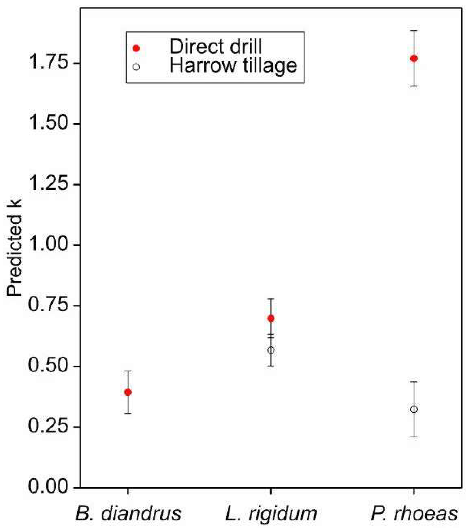
3.2. Relationships between Aggregation and Management Variables

The final model to predict the negative binomial parameter k was

$$\mathrm{E}\left(k\right)=\mathrm{Species}+\mathrm{Cultivation}+ \mathrm{Species}.\mathrm{Cultivation}+\mathsf{\epsilon },$$

(11)

where $\mathsf{\epsilon }$ is an error term which is assumed to be independent and identical. The interaction term is significant at (p = 0.01). The main effects are barely significant (Species, p = 0.06) and (Cultivation, p = 0.05). Papaver had significantly smaller predicted k values in harrow-tilled fields than in direct-drilled ones (Least Significant Difference, LSD = 0.66 at p = 0.05), indicating greater clumping. Lolium also had smaller values of k in harrow-tilled fields than in direct-drilled ones, but the difference was not statistically significant (LSD = 0.38 at p = 0.05). Under direct drilling, the predicted k was significantly smaller for Bromus than for Lolium (LSD = 0.40 at p = 0.05) and similarly, the value for Lolium was significantly smaller than for Papaver (LSD = 0.97). Under harrow tillage, k for Papaver was smaller than that for Lolium, but the difference was not statistically significant (LSD = 0.40 at p = 0.05) (Figure 1).

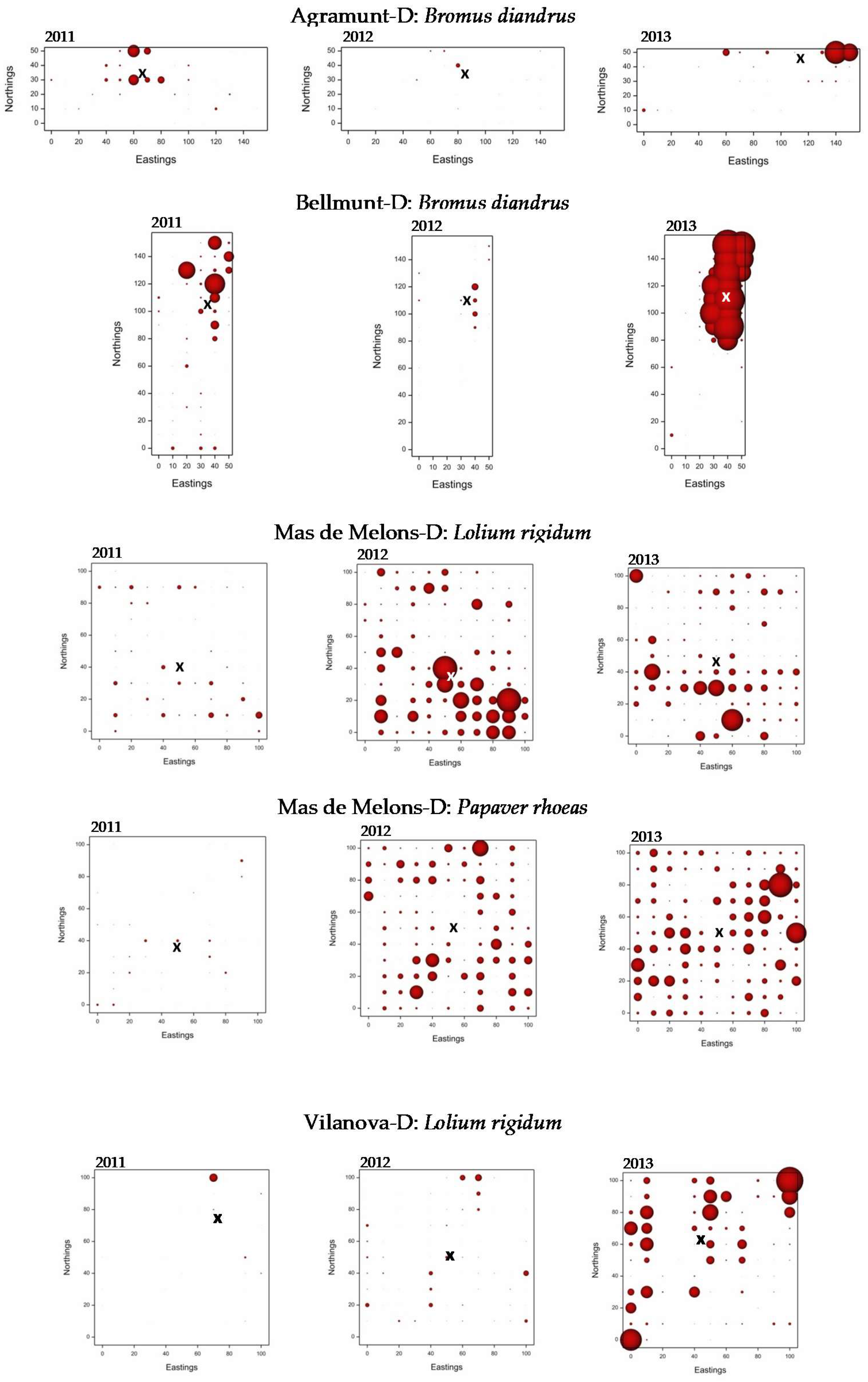
3.3. Weed Distribution Maps

Spatial patterns of the species in direct-drilled fields are shown in Figure 2. Bromus was the species with the most aggregated pattern. In Agramunt-D, it occurred predominantly in the northern half of the field, and its center of gravity shifted north-east-ward during the study. In Bellmunt-D, it occurred consistently in the north-eastern corner of the field, and though its cover varied from year to year, its center of gravity remained fairly stable. Lolium and Papaver were both homogeneously found throughout the fields in which they occurred, particularly at Mas de Melons-D.

Spatial patterns in harrow-tilled fields are shown in Figure 3. Lolium had a patchy distribution at Bellmunt-T. The patches occurred consistently near the northern edge of the field with the center of gravity shifting only a few meters east-ward in the course of the study. Some degree of stability over time can be seen also for Lolium at Vilanova-T in the eastern half of the field.

No differences in the aggregation pattern of the weeds were detected between the two forms of management. Such fluctuations of the weed cover between years in the same field can be attributed to the surveys themselves; some fields were sampled earlier some years than in others and so the plants were less developed. Also, some fields were either not sprayed with herbicide or the herbicide did not target the three species.

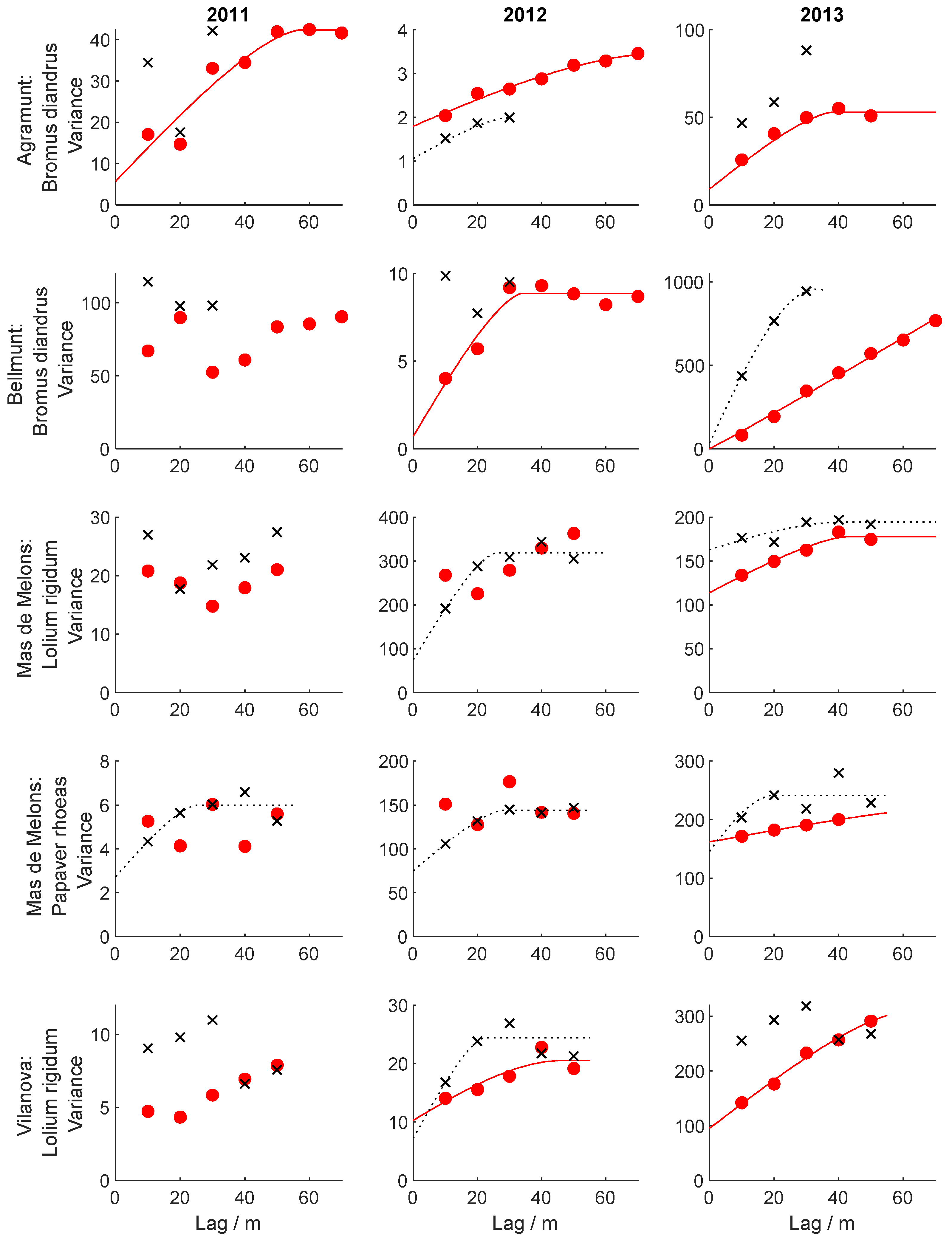
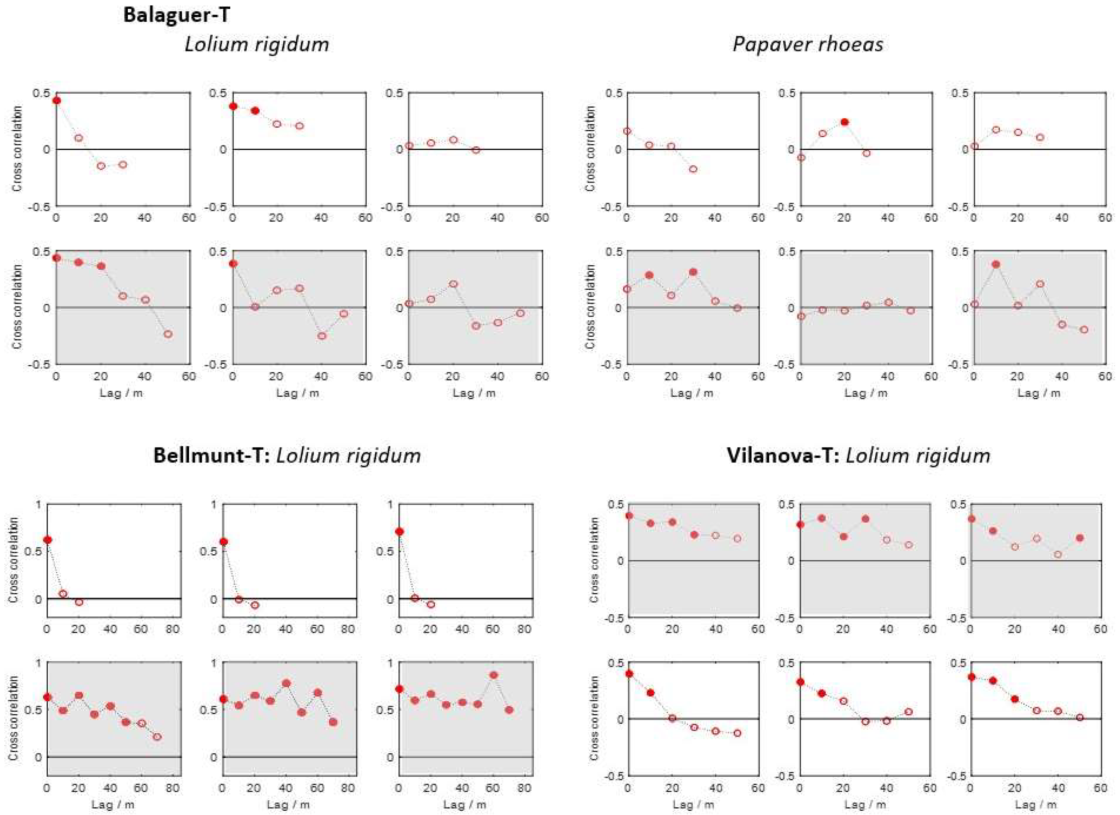
3.4. Spatial and Temporal Dependence of Weed Patterns

Experimental variograms were computed for each field for each year and species both parallel and perpendicular to the direction of traffic (Figure 4 and Figure 5 and

Table 4. Models fitted to the directional variograms (parallel, T, or perpendicular, P, to the field traffic) of the weed cover, with their parameter values for direct-drill (D) and harrow tillage (T) fields. The parameters are: $c_0$: nugget variance; $c$: sill; $a$: range; $g$: intensity of variation; $\alpha$: curvature.

Field	Species	Year	Direction	Model	c0	c	a/m	g	α
Agramunt-D	Bromus diandrus	2011	T	Circular	5.69	36.66	57.20
		2012	T	Spherical	1.80	1.69	81.90
			P	Circular	1.06	0.93	29.23
		2013	T	Circular	8.93	44.02	38.38
Bellmunt-D	Bromus diandrus	2012	T		0.71	8.15	33.93
		2013	T	Power	0			9.54	1.037
			P	Spherical	32.74	922.40	33.29
Mas de Melons-D	Lolium rigidum	2012	P	Circular	74.1	244.9	25.95
		2013	T	Circular	113.79	64.04	42.83
			P	Circular	162.80	31.70	42.20
	Papaver rhoeas	2011	P	Circular	2.73	3.27	25.16
		2012	T	Circular	75.08	69.02	28.07
		2013	T	Circular	161.88	61.10	78.00
			P	Spherical	146.00	96.00	20.20
Vilanova-D	Lolium rigidum	2012	T	Spherical	10.28	10.25	47.30
			P	Circular	7.20	17.20	22.20
		2013	T	Circular	94.80	212.60	60.20
Balaguer-T	Lolium rigidum	2011	P	Power	7.75			0.113	1.275
		2013	T	Power	2.02			0.0069	1.41
			P	Circular	0.12	0.98	31.00
	Papaver rhoeas	2012	T	Spherical	66.84	19.02	34.96
		2013	T	Circular	9.01	6.91	37.70
Bellmunt-T	Lolium rigidum	2011	T	Power	6.90			0.009	1.556
			P	Power	9.42			0.083	1.454
		2013	T	Circular	3.51	8.54	38.90
			P	Power	19.45			0.036	1.827
Vilanova-T	Lolium rigidum	2011	T	Spherical	4.85	18.59	46.5
			P	Spherical	13.23	11.90	68.00
		2012	P	Spherical	18.93	20.96	42.00
		2013	T	Circular	0.2816	5.088	18.38

). For six out of the 27 data sets it was not possible to fit spatial models, indicating that populations have no spatial dependence. Most of these sets came from fields where the weed cover was less than 1%. Seventeen out of 21 sets of data showed spatial dependence in the direction of the traffic and nine of them also showed dependence in the perpendicular direction. Four data sets showed dependence only in the perpendicular direction. Bromus and Papaver showed aggregation mainly in the direction of field traffic, whereas for Lolium there were no difference. Papaver showed the weakest spatial dependence of the three species, particularly at Mas de Melons-D, where in 2011 and 2012 the variogram models were almost wholly nugget variance. The limit of spatial dependence ranged from 22 m to 78 m and seems not to be related to the soil management.

The cross-correlation analyses showed that weed patches were stable in a few of the fields. In direct-drilled fields, only Bromus at Bellmunt-D had a significant correlation over time with a range extending to 40 m in the direction of traffic and almost 10 m perpendicular to it. The same species at Agramunt-D showed no stability between years. Lolium at Mas de Melons-D had a weak relation between year 2 and the other years, and at Vilanova-D only the first and second years were correlated for distances less than 10 m. Papaver at Mas de Melons-D showed correlation between some years (Figure 6). In harrow-tilled fields, in contrast, the covers of the three species were cross-correlated in most fields at least over two years and over longer distances. For example, the cross-correlation of Lolium extended to more than 50 m in the direction of traffic all years at Bellmunt-T and more than 10 m in both directions at Vilanova-T. At Balaguer-T, the cover of Lolium was also cross-correlated but to no more than 20 m and for only some of the years (Figure 7). Somewhat surprisingly, the cover of Papapver was not cross-correlated over any pair of years under either of the two forms of management.

4. Discussion

Recall that our aims were to assess the feasibility of mapping weeds for site-specific spraying and to discover whether there were differences in the patch stability of weed associated with cultivating by direct drilling or harrow tillage. We can summarize our findings as follows.

(1)

Weed cover varied substantially across fields with greater variation generally in direct-drilled fields.

(2)

Aggregation was greater for Bromus than for Lolium, and both were more aggregated than Papaver, but the degree of aggregation differed from year to year and between fields.

(3)

Papaver was more aggregated in harrow-tilled fields than in direct-drilled ones.

(4)

Spatial correlation was stronger in the direction of traffic than the perpendicular direction.

(5)

In a few of the fields the patches of weeds were stable from year to year; most of these fields were harrow-tilled.

(6)

The spatial stability was more pronounced in the direction of field traffic than in the perpendicular direction for all three species.

Both weed cover and degree of aggregation varied substantially from one year to the next. Weed populations and their spatial distribution reflect cropping history and current management. The fields surveyed had been managed in the same ways, either direct-drilled or harrow-tilled, for between 4 and 14 years. According to Swanton et al. [32], it may take 4–10 years for weed populations to reach equilibrium, and so, at least in part, the spatial distribution of the weeds is a consequence of soil management [33,34]. Bromus for example, is symptomatic of direct drilling [35], which creates favorable conditions for it [36].

According to the results, weed cover and location seem to have been modulated by management factors such as herbicides and rotation. The herbicides applied differed between fields and changed between years for the same field, and that might explain changes in weed cover. For example, at Balaguer-T the increase in weed densities observed in the second year is likely to have arisen because the weeds were resistant to the herbicide (the farmer told us), and the reduction observed in the third year seems to have been caused by the much greater efficacy of the new herbicide. The increased population of weeds at Vilanova-D arose because no grass–weed herbicide was used. Another source of variation of weed cover in the fields was crop rotation. The field of Mas de Melons-D was left fallow in 2012 and weeds would be favored by the absence of crop and lack of herbicide. Sampling time may also have been important in fields such as Agramunt-D, Bellmunt-T, and Bellmunt-D where the sampling was done earlier than usual the second year. These factors might have contributed to the variation in the weed cover from year to year.

Lolium but particularly Papaver were more aggregated (smaller k parameter) in the harrow-tilled fields than in the direct-drilled ones. We did not expect this because the absence of soil disturbance in direct-drilled fields should allow seeds to remain closer to their mother plants, resulting in a more patchy distribution (quadrats with large proportions of both small and large counts). One possible explanation is that direct-drilled fields had some sites and seasons where no herbicide was applied or, if an herbicide was applied, it did not target the species analyzed (Table 1). This allowed greater densities throughout the field that decreased the overall patchiness. The application or no application of herbicides may also explain the greater differences observed in the degree of weed aggregation between the direct-drilled fields (standard deviation of k = 0.62) compared with the harrow-tilled ones (standard deviation of k = 0.39).

The spatial dependence was stronger in the direction of the field traffic generally than in the perpendicular direction. The timing of seed shedding in all species is generally between June and July [37], coinciding with the harvest. Seeds of Papaver and Bromus that shed before harvest have a primary gravity-related dispersal in a limited space around the parent plants. Afterwards, they are dispersed in the direction of traffic by tillage, but the distance at which seeds move horizontally is limited to less than 2 m, and depends on the implement used [19,38]. Lolium does not shed its seeds spontaneously before harvest, and even after harvest most seeds are dispersed as clustered spikelets or spike fragments [39]. The seeds of Lolium and the seeds of Papaver and Bromus that are still on the plant can be dispersed by combine harvesters. Combine harvesters have been reported to move seeds in the machine direction from their source up to 18 m for L. rigidum [39] and up 30 m for Avena sterilis and A. fatua [40]. The smaller size and near-spherical shape of P. rhoeas seeds might make them less likely to be dispersed than larger seeds such as those of Bromus or seeds that remain attached to the spike at harvest time, such as those of Lolium. These large seeds can remain in the interior of combine harvesters after entering the headers only to be displaced further away in the direction of traffic, making a significant contribution to seed dispersal. For such seeds, primary dispersal might be less relevant. The role of the agricultural machinery on the intensity and direction of weed dispersal has been widely reported [41].

The shapes of weed patches can change (1), by expanding or shrinking radially as a result of population increase and dispersal (2), by intensifying or weakening as a result of an increase or decrease of the local population density without expanding or shrinking and (3), by shifting in space [14]. The statistical techniques we used to analyze the spatio-temporal processes are based on the calculation of cross-correlations in two directions across space and time. Correlations across space characterize shifts and expansions or shrinkages by comparison of a given sample location with its neighbors in different years and characterize intensification by comparison of each sample location with itself in different years [27]. All directions are accounted for, because all combinations of rows and columns are taken into account. The cross-correlation analyses did not detect temporal stability in most of the fields; only at Bellmunt-D with B. diandrus and Bellmunt-T and Vilanova-T with L. rigidum a significant stability was observed across years, being more perceptible in the direction of the field traffic and confirming the role of the traffic in modulating the spatial distribution of the weeds.

Some studies of spatial stability of weed patches in agricultural fields indicate that these remain remarkably stable over time [13,18,42,43]. However, absence of spatial stability [14,17,44] or stability over short times [11,12] have also been reported. Heiting et al. [14] attributed instability to both the dispersion mechanism of the species, being greater for weeds the seeds of which are dispersed by wind, and for species with sparser populations. The instability of patches in the fields we surveyed could be related to the concept of specialist and generalist plants. Species could be ranked along a specialist-to-generalist gradient based on their niche breadths [45]. Specialist species tend to be aggregated, whereas generalists and species that have an intermediate degree of habitat specialization tend to be segregated [46]. If we take into account the large distribution and abundance of B. diandrus, L. rigidum and P. rhoeas in the Mediterranean cereal fields [47], we can consider them to be generalists, and consequently, we can expect random aggregation patterns. Agronomic factors such as weed management rather than ecological-like niche requirements would mostly determine the location of these species. For example, in some of the fields that we studied (Agramunt-D, Bellmunt-D and Bellmunt-T) weed cover was greater towards the edges of the fields. Arable field edges have often been observed to support increased diversity and abundance of weeds compared with more central regions of the fields [48,49]. This is assumed to be due to both a reduction in agricultural inputs towards the field edge or spatial mass effects associated with dispersal of weeds from the surrounding landscape or both [50].

Aggregation was observed in most fields regardless of the soil management, but it did depend on both field and season. Herbicide applications, crop rotation, and traffic seem to affect weed populations strongly within fields, regardless of the soil management. The instability of the patches and the variation observed between years in the weed cover do not limit the application of site-specific weed control of these weeds in conservation tillage systems. The instability limits only the more-than-one-year-use of weed distribution maps based on discrete sampling. Other technologies such as real-time weed detection with optical sensors and on-board computer analyses can be more appropriate. We recommend that future research on site-specific weed management should be addressed to improve the detection of weeds in order to increase the efficacy of the control, particularly in CA systems with direct drill, with an enhanced reliance on herbicides. It is expected that this ground-based continuous sampling technology, neither labor-intensive nor time-consuming, can become more affordable in the future with the spread of its use.

References

1. Llewellyn, R.S.; Ronning, D.; Ouzman, J.; Walker, S.; Mayfield, A.; Clarke, M. Impact of Weeds on Australian Grain Production: The Cost of Weeds to Australian Grain Growers and the Adoption of Weed Management and Tillage Practices; Report for GRDC; CSIRO: Canberra, Australia, 2016; p. 112. [Google Scholar]
2. Izquierdo, J.; Recasens, J.; Fernández-Quintanilla, C.; Gill, G. Effects of crop and weed densities on the interactions between barley and Lolium rigidum in several Mediterranean locations. Agronomie 2003, 23, 529–536. [Google Scholar] [CrossRef]
3. Torner, C.; González-Andújar, J.L.; Fernández-Quintanilla, C. Wild oat (Avena-sterilis L.) competition with winter barley: Plant-density effects. Weed Res. 1991, 31, 301–307. [Google Scholar] [CrossRef]
4. García, A.L.; Torra, J.; Royo-Esnal, A.; Cantero-Martínez, C.; Recasens, J. Integrated management of Bromus diandrus in dryland cereal fields under no-till. Weed Res. 2014, 54, 408–417. [Google Scholar]
5. Wilson, B.J.; Wright, K.J.; Brain, P.; Clements, M.; Stephens, E. Predicting the competitive effects of weed and crop density on weed biomass, weed seed production and crop yield in wheat. Weed Res. 1995, 35, 265–278. [Google Scholar] [CrossRef]
6. Gerhards, R.; Sokefeld, M.; Schulze, L.K.; Mortensen, D.A.; Kuhbauch, W. Site-specific weed control in winterwheat. J. Agron. Crop Sci. 1997, 178, 219–225. [Google Scholar] [CrossRef]
7. Gerhards, R.; Christensen, S. Real-time weed detection, decision making and patch spraying in maize, sugarbeet, winter wheat and winter barley. Weed Res. 2003, 43, 385–392. [Google Scholar] [CrossRef]
8. Peteinatos, G.G.; Weis, M.; Andújar, D.; Ayala, V.R.; Gerhards, R. Potential use of ground-based sensor technologies for weed detection. Pest Manag. Sci. 2014, 70, 190–199. [Google Scholar] [CrossRef]
9. López-Granados, F.; Torres-Sánchez, J.; De Castro, A.I.; Serrano-Pérez, A.; Mesas-Carrascosa, F.J.; Peña, J.M. Object-based early monitoring of a grass weed in a grass crop using high resolution UAV imagery. Agron. Sustain. Dev. 2016, 36, 67. [Google Scholar] [CrossRef]
10. Mink, R.; Dutta, A.; Peteinatos, G.G.; Sokefeld, M.; Engels, J.J.; Hahn, M.; Gerhards, R. Multi-temporal site-specific weed control of Cirsium arvense (L.) Scop. and Rumex crispus L. in maize and sugar beet using unmanned aerial vehicle based mapping. Agric.-Basel 2018, 8, 65. [Google Scholar] [CrossRef] [Green Version]
11. Johnson, G.A.; Mortensen, D.A.; Gotway, C.A. Spatial and temporal analysis of weed seedling populations using geostatistics. Weed Sci. 1996, 44, 704–710. [Google Scholar] [CrossRef]
12. Colbach, N.; Forcella, F.; Johnson, G.A. Spatial and temporal stability of weed populations over five years. Weed Sci. 2000, 48, 366–377. [Google Scholar] [CrossRef]
13. Dieleman, J.A.; Mortensen, D.A.; Martin, A.R. Influence of velvetleaf (Abutilon theophrasti) and common sunflower (Helianthus annuus) density variation on weed management outcomes. Weed Sci. 1999, 47, 81–89. [Google Scholar] [CrossRef]
14. Heijting, S.; Van der Werf, W.; Stein, A.; Kropff, M.J. Are weed patches stable in location? Application of an explicitly two-dimensional methodology. Weed Res. 2007, 47, 381–395. [Google Scholar] [CrossRef]
15. Calha, I.M.; Sousa, E.; González-Andújar, J.L. Infestation maps and spatial stability of main weed species in maize culture. Planta Daninha 2014, 32, 275–282. [Google Scholar] [CrossRef] [Green Version]
16. Castillejo-González, I.L.; de Castro, A.I.; Jurado-Expósito, M.; Peña, J.M.; García-Ferrer, A.; López-Granados, F. Assessment of the persistence of Avena sterilis L. patches in wheat fields for site-specific sustainable management. Agron.-Basel 2019, 9, 30. [Google Scholar] [CrossRef] [Green Version]
17. Izquierdo, J.; Blanco-Moreno, J.M.; Chamorro, J.; Recasens, J.; Sans, F.X. Spatial distribution and temporal stability of postrate knotweed (Polygonum aviculare) and corn poppy (Papaver rhoeas) seed bank in a cereal field. Weed Sci. 2009, 57, 505–511. [Google Scholar] [CrossRef]
18. Wilson, B.J.; Brain, P. Long-term stability of distribution of Alopecurus myosuroides Huds. within cereal fields. Weed Res. 1991, 31, 367–373. [Google Scholar] [CrossRef]
19. Marshall, E.J.P.; Brain, P. The horizontal movement of seeds in arable soil by different soil cultivation methods. J. Appl. Ecol. 1999, 36, 443–454. [Google Scholar] [CrossRef]
20. Cantero-Martínez, C.; Angas, P.; Lampurlanés, J. Growth, yield and water productivity of barley (Hordeum vulgare L.) affected by tillage and N fertilization in Mediterranean semiarid, rainfed conditions of Spain. Field Crop Res. 2003, 84, 341–357. [Google Scholar] [CrossRef]
21. Nichols, V.; Verhulst, N.; Cox, R.; Govaerts, B. Weed dynamics and conservation agriculture principles: A review. Field Crops Res. 2015, 183, 56–68. [Google Scholar] [CrossRef] [Green Version]
22. Mulugeta, D.; Boerboom, C.M. Seasonal abundance and spatial pattern of Setaria faberi, Chenopodium album, and Abutilon theophrasti in reduced-tillage soybeans. Weed Sci. 1999, 47, 95–106. [Google Scholar] [CrossRef]
23. Pollnac, F.W.; Rew, L.J.; Maxwell, B.D.; Menalled, F.D. Spatial patterns, species richness and cover in weed communities of organic and conventional no-tillage spring wheat systems. Weed Res. 2008, 48, 398–407. [Google Scholar] [CrossRef]
24. Hess, M.; Barralis, G.; Bleiholder, H.; Buhr, L.; Eggers, T.H.; Hack, H.; Stauss, R. Use of the extended BBCH scale—General for the descriptions of the growth stages of mono- and dicotyledonous weed species. Weed Res. 1997, 37, 433–441. [Google Scholar] [CrossRef]
25. Ludwig, J.A.; Reynolds, J.F. Chapter 3: Distribution methods. In Statistical Ecology: A Primer on Methods and Computing; John Wiley & Sons, Ltd.: New York, NY, USA, 1998; p. 362. [Google Scholar]
26. Payne, R.W. (Ed.) The Guide to Genstat Release 19—Part 2: Statistics; VSN International: Hemel Hempsted, UK, 2018. [Google Scholar]
27. Webster, R.; Oliver, M.A. Geostatistics for Environmental Scientists, 2nd ed.; John Wiley & Sons, Ltd.: New York, NY, USA, 2007; p. 330. [Google Scholar]
28. Kotwicki, S.; Lauth, R.R. Detecting temporal trends and environmentally-driven changes in the spatial distribution of bottom fishes and crabs on the eastern Bering Sea shelf. Deep-Sea Res. Pt II 2013, 94, 231–243. [Google Scholar] [CrossRef]
29. MATLAB 2018a; The MathWorks, Inc.: Natick, MA, USA, 2018.
30. Monaghan, N.M. Biology and control of Lolium rigidum as a weed of wheat. Weed Res. 1980, 20, 117–121. [Google Scholar] [CrossRef]
31. Riba, F.; Recasens, J.; Taberner, A. Flora arvense de los cereales de invierno de Catalunya (I). In Proceedings of the Actas de la Reunión 1990 de la Sociedad Española de Malherbología, Madrid, Spain, 11–12 December 1990; pp. 239–246. [Google Scholar]
32. Swanton, C.J.; Clements, D.R.; Derksen, D.A. Weed succession under conservation tillage: A hierarchical framework for research and management. Weed Technol. 1993, 7, 286–297. [Google Scholar] [CrossRef]
33. Campiglia, E.; Radicetti, E.; Mancinelli, R. Floristic composition and species diversity of weed community after 10 years of different cropping systems and soil tillage in a Mediterranean environment. Weed Res. 2018, 58, 273–283. [Google Scholar] [CrossRef]
34. Alarcón, R.; Hernández-Plaza, E.; Navarrete, L.; Sánchez, M.J.; Escudero, A.; Hernanz, J.L.; Sánchez-Girón, V.; Sánchez, A.M. Effects of no-tillage and non-inversion tillage on weed community diversity and crop yield over nine years in a Mediterranean cereal-legume cropland. Soil Till. Res. 2018, 179, 54–62. [Google Scholar] [CrossRef]
35. Moreno, F.; Arrué, J.L.; Cantero-Martínez, C.; López, M.V.; Murillo, J.M.; Sombrero, A.; López-Garrido, R.; Madejón, E.; Moret, D.; Álvaro-Fuentes, J. Conservation agriculture under Mediterranean conditions in Spain. In Biodiversity, Biofuels, Agroforestry and Conservation Agriculture. Sustainable Agriculture Reviews; Lichtfouse, E., Ed.; Springer: London, UK, 2010; Volume 5, pp. 175–193. [Google Scholar]
36. Recasens, J.; García, A.L.; Cantero-Martínez, C.; Torra, J.; Royo-Esnal, A. Long-term effect of different tillage systems on the emergence and demography of Bromus diandrus in rainfed cereal fields. Weed Res. 2016, 56, 31–40. [Google Scholar] [CrossRef] [Green Version]
37. Westerman, P.R.; Atanackovic, V.; Royo-Esnal, A.; Torra, J. Differential weed seed removal in dryland cereals. Arthropod-Plant Inte. 2012, 6, 591–599. [Google Scholar] [CrossRef]
38. Rew, L.J.; Cussans, G.W. Horizontal movement of seeds following tine and plough cultivation: Implications for spatial dynamics of weed infestations. Weed Res. 1997, 37, 247–256. [Google Scholar] [CrossRef]
39. Blanco-Moreno, J.M.; Chamorro, L.; Masalles, R.M.; Recasens, J.; Sans, F.X. Spatial distribution of Lolium rigidum seeds following seed dispersal by combine harvesters. Weed Res. 2004, 44, 375–387. [Google Scholar] [CrossRef]
40. Barroso, J.; Navarrete, L.; Del Arco, M.J.S.; Fernández-Quintanilla, C.; Lutman, P.J.W.; Perry, N.H.; Hull, R.I. Dispersal of Avena fatua and Avena sterilis patches by natural dissemination, soil tillage and combine harvesters. Weed Res. 2006, 46, 118–128. [Google Scholar] [CrossRef]
41. Petit, S.; Alignier, A.; Colbach, N.; Joannon, A.; Le Coeur, D.; Thenail, C. Weed dispersal by farming at various spatial scales. A review. Agron. Sustain. Dev. 2013, 33, 205–217. [Google Scholar] [CrossRef]
42. Barroso, J.; Fernández-Quintanilla, C.; Ruiz, D.; Hernaiz, P.; Rew, R.J. Spatial stability of Avena sterilis ssp ludoviciana populations under annual applications of low rates of imazamethabenz. Weed Res. 2004, 44, 178–186. [Google Scholar] [CrossRef]
43. Blanco-Moreno, J.M.; Chamorro, L.; Sans, F.X. Spatial and temporal patterns of Lolium rigidum-Avena sterilis mixed populations in a cereal field. Weed Res. 2006, 46, 207–218. [Google Scholar] [CrossRef]
44. Wyse-Pester, D.Y.; Wiles, L.J.; Westra, P. Infestation and spatial dependence of weed seedling and mature weed populations in corn. Weed Sci. 2002, 50, 54–63. [Google Scholar] [CrossRef]
45. Fried, G.; Petit, S.; Reboud, X.A. Specialist-generalist classification of the arable flora and its response to changes in agricultural practices. BMC Ecol. 2010, 10, 20. [Google Scholar] [CrossRef] [Green Version]
46. Petit, S.; Fried, G. Patterns of weed co-occurrence at the field and landscape level. J. Veg. Sci. 2012, 23, 1137–1147. [Google Scholar] [CrossRef]
47. Holm, L.G.; Doll, J.; Holm, E.; Pancho, J.V.; Herberger, J.P. World Weeds: Natural Histories and Distribution; John Wiley & Sons, Ltd.: New York, NY, USA, 1997; p. 1152. [Google Scholar]
48. Wilson, P.J.; Aebischer, N.J. The distribution of dicotyledonous arable weeds in relation to distance from the field edge. J. Appl. Ecol. 1995, 32, 295–310. [Google Scholar] [CrossRef]
49. Alignier, A.; Petit, S.; Bohan, D.A. Relative effects of local management and landscape heterogeneity on weed richness, density, biomass and seed rain at the country-wide level, Great Britain. Agr. Ecosyst. Environ. 2017, 246, 12–20. [Google Scholar] [CrossRef]
50. Metcalfe, H.; Hassall, K.; Boinot, S.; Storkey, J. The contribution of spatial mass effects to plant diversity in arable fields. J. Appl. Ecol. 2019, 56, 1560–1574. [Google Scholar] [CrossRef] [PubMed]
Figure 1. Predicted values of the k parameter of the negative binomial distribution when fitted to data on the weed cover of B. diandrus, L. rigidum and P. rhoeas from seven fields in North-eastern Spain measured over the 3 years. The bars indicate the standard errors. The numbers of field by season observations for each species and tillage combination are as follows. For direct-drilled fields: B. diandrus, n = 6, L. rigidum, n = 6 and P. rhoeas, n = 3 and for harrow-tilled fields: L. rigidum, n = 9 and P. rhoeas, n = 3.
Agronomy 10 00452 g001
Figure 2. Maps of weed cover (%) with centers of gravity (x) in the fields with direct drilling (D). Circle sizes are proportional to the percentages of weed cover: Agronomy 10 00452 i001 100% Agronomy 10 00452 i002 50% Agronomy 10 00452 i003 25% Agronomy 10 00452 i004 10%.
Agronomy 10 00452 g002
Figure 3. Maps of weed cover (%) with centers of gravity (x) in the fields with harrow tillage (T). Circle sizes are proportional to the percentage of weed cover: Agronomy 10 00452 i005 100% Agronomy 10 00452 i006 50% Agronomy 10 00452 i007 25% Agronomy 10 00452 i008 10%.
Agronomy 10 00452 g003
Figure 4. Empirical variograms with fitted models (solid and dotted lines) for direct-drilled sites. Variograms with lag distance in the direction of traffic are shown by the red discs, and those with lag distance perpendicular to field traffic are shown by the black crosses. The model parameters are given in Table 4. Where no line appears, a model could not be fitted.
Agronomy 10 00452 g004
Figure 5. Empirical variograms with fitted models (solid and dotted lines) for harrow-tilled sites. Variograms with lag distance in the direction of traffic are shown by the red discs, and those with lag distance perpendicular to traffic are shown by the black crosses. The model parameters are given in Table 4. Where no line appears, a model could not be fitted.
Agronomy 10 00452 g005
Figure 6. Cross-correlation of weed cover between years of the main weeds in the direct drilling fields (D). First row graphs: N–S direction, second row: E–W direction. Rows with grey background: direction of traffic. First column graphs: cross-correlation years 1 and 2, second column years 1 and 3 and third column years 2 and 3. Solid symbols mean that cross-correlation is significantly different from random.
Agronomy 10 00452 g006
Figure 7. Cross-correlation of weed cover between years of the main weeds in the harrow-tilled fields (T). First row graphs: N–S direction, second row: E–W direction. Rows with grey background: direction of traffic. First column graphs: cross-correlation years 1 and 2, second column years 1 and 3 and third column years 2 and 3. Solid symbols mean that cross-correlation is significantly different from random.
Agronomy 10 00452 g007