Bottom-Up Assessment of Climate Risk and the Robustness of Proposed Flood Management Strategies in the American River, CA


1
Wicked Water Strategies, Bend, OR 97701, USA
2
Department of Statistics, Oregon State University, Corvallis, OR 97731, USA
3
Stockholm Environmental Institute, 110231 Bogotá D.C., Colombia
*
Author to whom correspondence should be addressed.
Water 2020, 12(3), 907; https://doi.org/10.3390/w12030907
Submission received: 15 January 2020
/
Revised: 21 February 2020
/
Accepted: 14 March 2020
/
Published: 23 March 2020
(This article belongs to the Special Issue Process Based Modelling of Natural and Distributed Flood Control Measures)
Abstract
:The hydrologic nonstationarity and uncertainty associated with climate change requires new decision-making methods to incorporate climate change impacts into flood frequency and flood risk analyses. To aid decision-making under climate change, we developed a bottom-up approach for assessing the performance of flood management systems under climate uncertainty and nonstationarity. The developed bottom-up approach was applied to the American River, CA, USA flood management system by first identifying the sensitivity and vulnerability of the system to different climates. To do this, we developed a climate response surface by calculating and plotting Expected Annual Damages (EAD, $/year) under different flood regimes. Next, we determined a range of plausible future climate change and flood frequency scenarios by applying Bayesian statistical methods to projected future flows derived from a Variable Infiltration Capacity (VIC) model forced with Global Circulation Model (GCM) output. We measured system robustness as the portion of plausible future scenarios under which the current flood system could meet its performance goal. Using this approach, we then evaluated the robustness of four proposed management strategies in the 2012 Central Valley Flood Protection Plan in terms of both flood risk and cost-effectiveness, to assess the performance of the strategies in the face of climate risks. Results indicated that the high sensitivity of the expected damages to changes in flood regimes makes the system extremely vulnerable to a large portion of the plausible range of future flood conditions. The management strategy that includes a combination of nature-based flood management actions along with engineered structures yields the greatest potential to increase system robustness in terms of maintaining EAD below an acceptable risk threshold. However, this strategy still leaves the system vulnerable to a wide range of plausible future conditions. As flood frequency regimes increase in intensity from the current conditions, the cost-effectiveness of the management strategies increases, to a point, before decreasing. This bottom up analysis demonstrated a viable decision-making approach for water managers in the face of uncertain and changing future conditions. Neglecting to use such an approach and omitting climate considerations from water resource planning could lead to strategies that do not perform as expected or which actually lead to mal-adaptations, increasing vulnerability to climate change.
1. Introduction
Scientists and managers currently lack reliable climate projections at the temporal and spatial resolution required to perform traditional flood risk analyses. Furthermore, there is no consensus on methods to incorporate multiple, uncertain future scenarios into such analyses. Climate model output has served as the starting point and basis of most studies of climate risk [1,2,3]. However, the output from climate models is often ill-suited for this role for several interrelated reasons that include:
- Cascading, increasing uncertainty through bias correction and downscaling to achieve desired spatial and temporal resolution [8].
Importantly, advances in modeling and downscaling techniques will not ameliorate the concerns listed above. While new generations of GCMs, Coupled Model Intercomparison Project (CMIP) output, Regional Climate Models (RCMs), and downscaling techniques all possess the potential to better characterize uncertainty, these new models and techniques will by no means eliminate uncertainty, and instead may increase uncertainty in future climate projections [9,10]. Current approaches to flood frequency analysis (e.g., Bulletin 17B used in the United States [11]), that rely on a single, reliable, long-term hydrologic record and assume stationarity are ill-suited for assessing flood risk using multiple, highly uncertain climate change projections.
To date, top-down, scenario-led impact assessments have dominated thinking on climate change impacts and evaluation of potential adaptation measures (e.g., [1,2,3]). However, the dependence of these approaches on a small set of deeply uncertain, downscaled GCM output limits their ability to reliably assess the full range of future flood risk. Currently, no agreement exists on a universally appropriate method to temporally and spatially downscale GCM output to the resolution required for flood frequency analysis (e.g., catchment scale and daily or sub-daily time step) [12,13]. At the same time, the choice of downscaling method can have significant implications for flood frequency analysis [6]. Alternatively, RCMs can be used to indirectly derive regional climate from GCM output, though RCMs have their own issues [14]. In either case, calculating the resulting streamflow requires further modeling efforts to force hydrologic models with the output from the climate models. As a result, uncertainty is cascaded down the various steps reaching the point where the streamflow impacts can span wide, confounding ranges, which may even include opposite signs, e.g., an increase or decrease in flood magnitude [8,15]. Few studies take the additional step of combining the hydrologic projections with damage projections, regardless of how these damages are characterized, in order to assess vulnerability and flood risk [8,15], which adds another layer of uncertainty to the results. Demonstrating an approach to accomplish this is the primary innovation of this effort.
Approaching flood risk assessment from the bottom-up can overcome some of the limitations of top-down decision-making. With bottom-up approaches, assessments are tailored to address a specific flood management decision within the limitations of the available data. Bottom-up approaches take several names and forms, including: Scenario-neutral approaches [15], decision scaling [16,17], climate risk informed decision analysis [18,19], and robust decision-making [8,20]. These approaches reverse the order of typical impact and vulnerability assessment used in top-down approaches, as well as the order in which projected hydrologic information is used to inform decision-making. Top-down approaches first generate a limited set of downscaled climate scenarios from which to assess impacts and then vulnerability to those limited scenarios. In contrast, bottom-up assessments generally start with an identified management concern, around which system sensitivity and vulnerability to climate are characterized. Bottom-up approaches acknowledge the limits of uncertain climate model output and downscaling approaches, and as such they only consider GCMs in the later stages of the risk assessment process, alongside other available climate data, such as observations and paleontological data.
We present a methodology for bottom-up assessment of flood damages based on existing frameworks [16,21] that require first defining the decision context for assessing climate impacts on water systems. The decision context refers to identifying the assessment goals and relevant parameters in the context of a specific management or policy decision, and it is established before choosing and analyzing models and data [21]. Focusing on the specific management decision or policy at hand, bottom-up approaches scale and tailor climate information to inform that decision, usually through a sensitivity and vulnerability analysis. We began our analysis with a sensitivity and vulnerability assessment that does not consider climate projections, but is intended to help water managers better understand the hydrologic conditions that push their systems into a vulnerable state. For this bottom-up flood risk assessment, sensitivity is defined in terms of how much Expected Annual Damages (EAD) change under different climatic conditions. A system’s vulnerability to exceeding an acceptable flood risk is defined by the extent to which a system is unable to maintain EAD below a threshold risk level. As part of the sensitivity and vulnerability analyses, several studies [15,16,22] have developed functions to describe climate response (e.g., increase in peak flows) as a function of changes in mean annual precipitation and seasonal variation. We took this work a step further by describing climate response in terms of flood risk, a function of both changes in peak flows and the damages associated with those flows [23]. While other flood damage assessment techniques exist, with active research on the topic ongoing, this is not the focus of this effort. Rather, the proposed innovation can be applied to any existing or emerging technique.
The climate response surfaces, describing sensitivity and vulnerability, in combination with plausible climate impacts, can be used to compare the future performance of different management actions and determine the climate scenarios that favor certain strategies over others. The metrics used to assess system performance differ in bottom-up and top-down approaches. Top-down approaches tend to seek an optimum solution based on the probability of future scenarios occurring and the expected value of different decisions under those scenarios. However, in the face of uncertain climatic changes, rather than seeking optimal performance, a growing body of literature advocates for seeking robust strategies that perform reasonably well over a wide range of uncertain, yet plausible future scenarios [7,8,20,24,25,26]. By using robustness criterion in combination with a vulnerability and impact assessment, managers can evaluate: Whether actions towards adaptations are needed [16], the conditions that cause a particular decision to be favored over another [22], or the robustness of a policy [15].
We present a climate risk and adaptation assessment of the flood management system in the American River basin, CA, USA with the objectives of: (1) Developing a bottom-up methodology for the assessment of flood management decisions in which uncertainty and nonstationarity of flood frequencies are directly considered and (2) applying the methodology to the flood management system in the American River to characterize its vulnerabilities to flood damages under different climate and management scenarios. This second objective aims to respond directly to specific planning efforts conducted as part of the Central Valley Flood Protection Plan (CVFPP). Using a bottom-up approach, we began by framing this decision context around a key question water resources managers have been investigating [27]: Given climate change, what is the most robust strategy to take for managing flood risk in the American River basin? To inform this decision, we (1) identified the sensitivity of the American River flood system to different climates, defined in terms of changes in EAD; (2) identified a vulnerability range of flood regimes under which the current system cannot maintain flood risk (EAD) below an acceptable threshold; (3) determined potential changes in flood frequency and flood risk under climate change by stochastically generating a set of plausible future flood regimes; and (4) evaluated the robustness of the flood management scenarios under plausible future conditions in terms of their ability to maintain flood risk below a threshold EAD and maintain a benefit-cost ratio (BCR) above a cost-effectiveness threshold.
Study Area: American River Basin, CA, USA
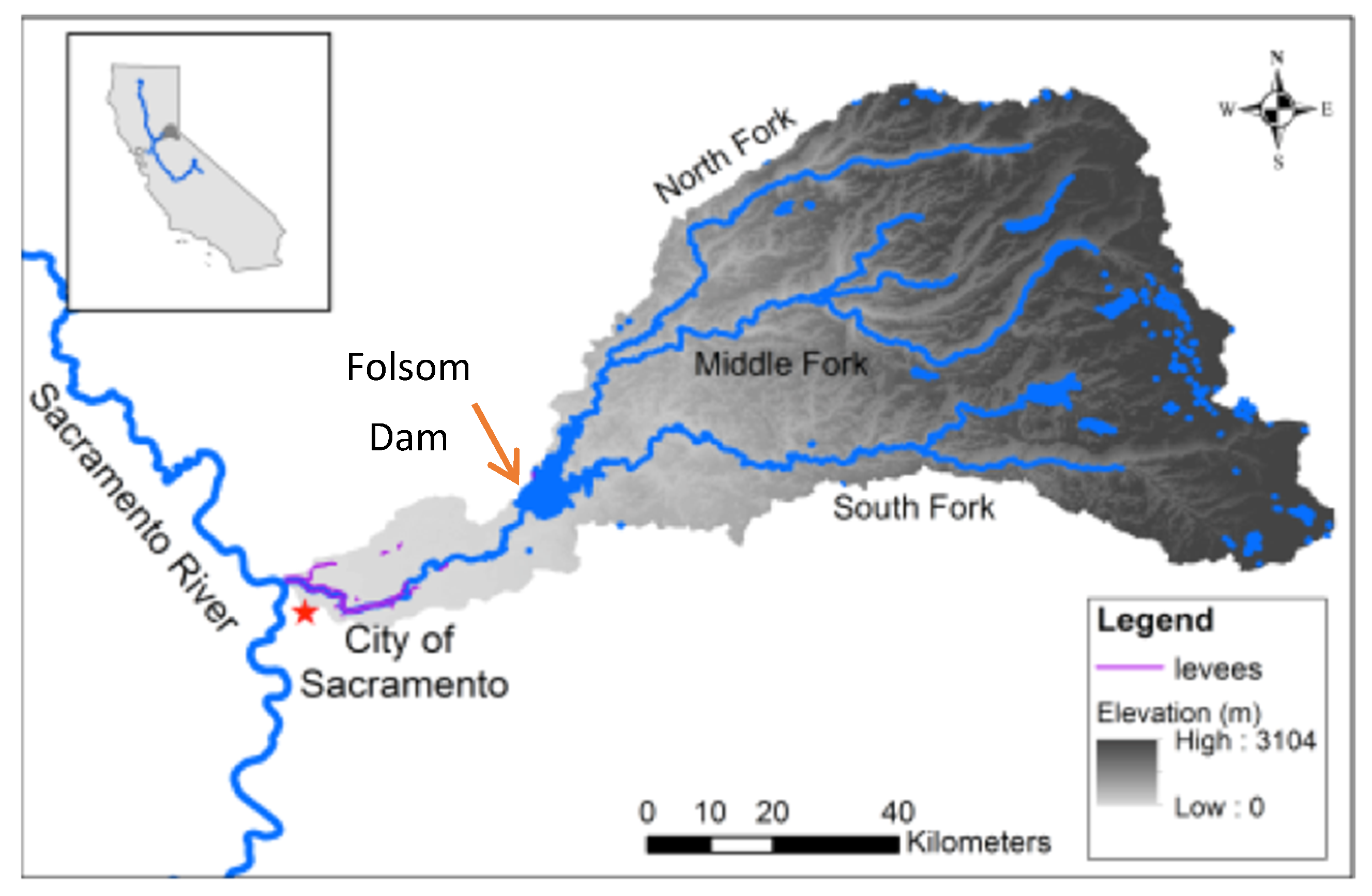
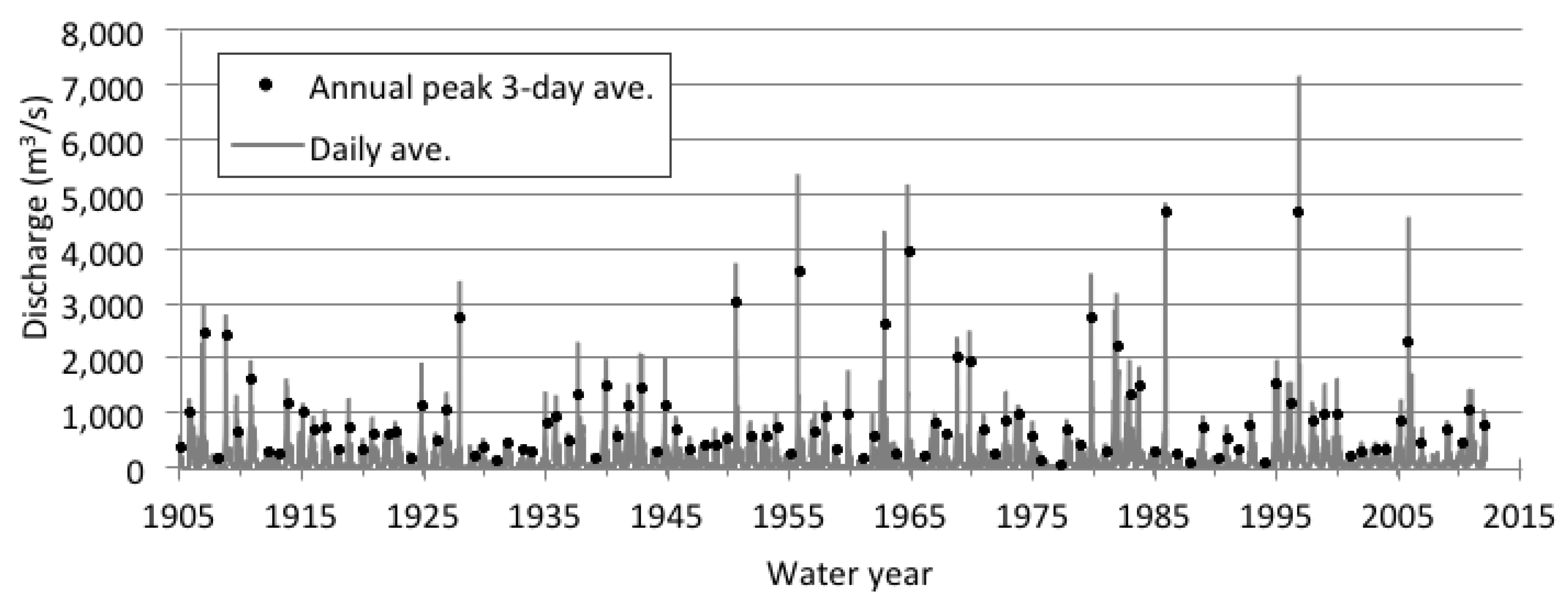
From its headwaters in the western slopes of the Sierra Nevada mountain range in Northern California, the American River flows southwest towards its confluence with the Sacramento River at the City of Sacramento (Figure 1). This study focused on flood risk in the highly populated portion of the basin to the south of the American River. The American River drains an area of 4975 km2, from elevations of 3170 m. along the Sierra crest to 7 m. above sea level at the confluence with the Sacramento River. Forty percent of the basin lies above the snowline, which occurs at an elevation of approximately 1500 m. The basin has a Mediterranean climate, with 90% of annual precipitation falling in 2–3 winter months [3]. Wintertime rainfall and snowmelt runoff comprises about two-thirds of the American River streamflow, with less than one-third derived from springtime snowmelt runoff [28]. The American River experiences large variations in annual precipitation and streamflow (Figure 2). Much of this variation results from water years that include a few large storms fueled by the landfall of atmospheric rivers. Known informally as “Pineapple Express” storms in the Pacific region, these events produce a narrow corridor of concentrated moisture that travels northeast over the Pacific Ocean from an area near Hawaii to California [29]. As the moist air and orography interact over land, the events can generate substantial portions of a basin’s annual precipitation and runoff (e.g., up to 50% for California [29]) over the course of a few days, often leading to substantial flood hazards.
The history of flooding on the American and Sacramento Rivers pre-dates European settlement; In 1808 the Spanish explorer Ensign Gabriel Moraga observed evidence that the rivers created “one immense sea, leaving only scattered eminences which art of nature have produced, as so many islets or spots of refuge” (in [30]). Attempts to control the floodwaters of the American River necessarily coincided with settlement and continue to this day. The State Plan for Flood Control (SPFC) descriptive document produced in 2010 [31], represented California’s first large-scale coordinated effort to manage floods at the state level. The SPFC is comprised of: Facilities (levees, weirs, dams, pumping plants, bypass basins, etc.); lands (fee title, easements, and land use agreements); operations and maintenance (O&M) requirements of SPFC facilities, conditions (terms, Memorandums of Understanding, regulations, etc.); and programs and plans. Major SPFC works in the American River basin include Folsom Reservoir and Dam, located at the confluence of the American River’s two main tributaries (Figure 1); levees on both banks of much of lower portions of the river below Folsom; and three pumping plants [32]. About the SPFC, the California Department of Water Resources (CA-DWR) [32] has concluded that:
- It has prevented billions of dollars in flood damages since its inception;
- some SPFC facilities face an unacceptably high chance of failure; and
- an unintended consequence of the long-term effort to reduce flooding is that development and population growth behind levee-protected areas have increased flood damages over time.
Thus, although the probability of flooding has decreased, the damages when floods occur are much higher today than they were in the past, resulting in a net long-term increase in flood risk [27]. The City of Sacramento faces some of the highest flood risk in the United States and the developed world [33], which is one of the reasons many prior research efforts [23,28,34,35] and financial investments have attempted to help manage flood risk in the American River basin. In this study, we expanded upon previous flood management work in the basin to include a bottom-up climate impact assessment.
2. Data and Methods
The developed methodology for conducting the climate risk assessment is in line with other bottom-up studies, but it uniquely tailors the approach to the specific decision context in the American River basin, uses only existing models and available data, and incorporates a Bayesian approach to developing a plausible range of future climates. We undertook the following steps to conduct a bottom-up risk assessment of a retrospective decision regarding future flood management strategies for the American River basin:
- Establish the decision context
- Assess the sensitivity of the system to changes in climate and flood regimes
- Assess the vulnerability of the system to flood regime changes
- Determine a plausible range of future flood regimes
- Assess the robustness of management strategies
2.1. Establishment of the Decision Context
In response to increasing flood damages, highlighted during flooding in the 1990s, the California State Legislature directed the CA-DWR to prepare a Central Valley Flood Protection Plan (CVFPP) and supporting documentation [27] as an enhancement to the SPFC. The primary goal of the 2012 CVFPP is to improve flood risk management, though the plan also includes supplemental goals to improve operations and maintenance of project facilities, promote ecosystem functions, improve institutional support, and promote multi-benefit projects. It is important to note that the current study is designed to supplement, not critique the CVFPP. As such, the CVFPP provided the decision context for the proposed innovation related to adapting flood management plans more generally to changing climatic conditions.
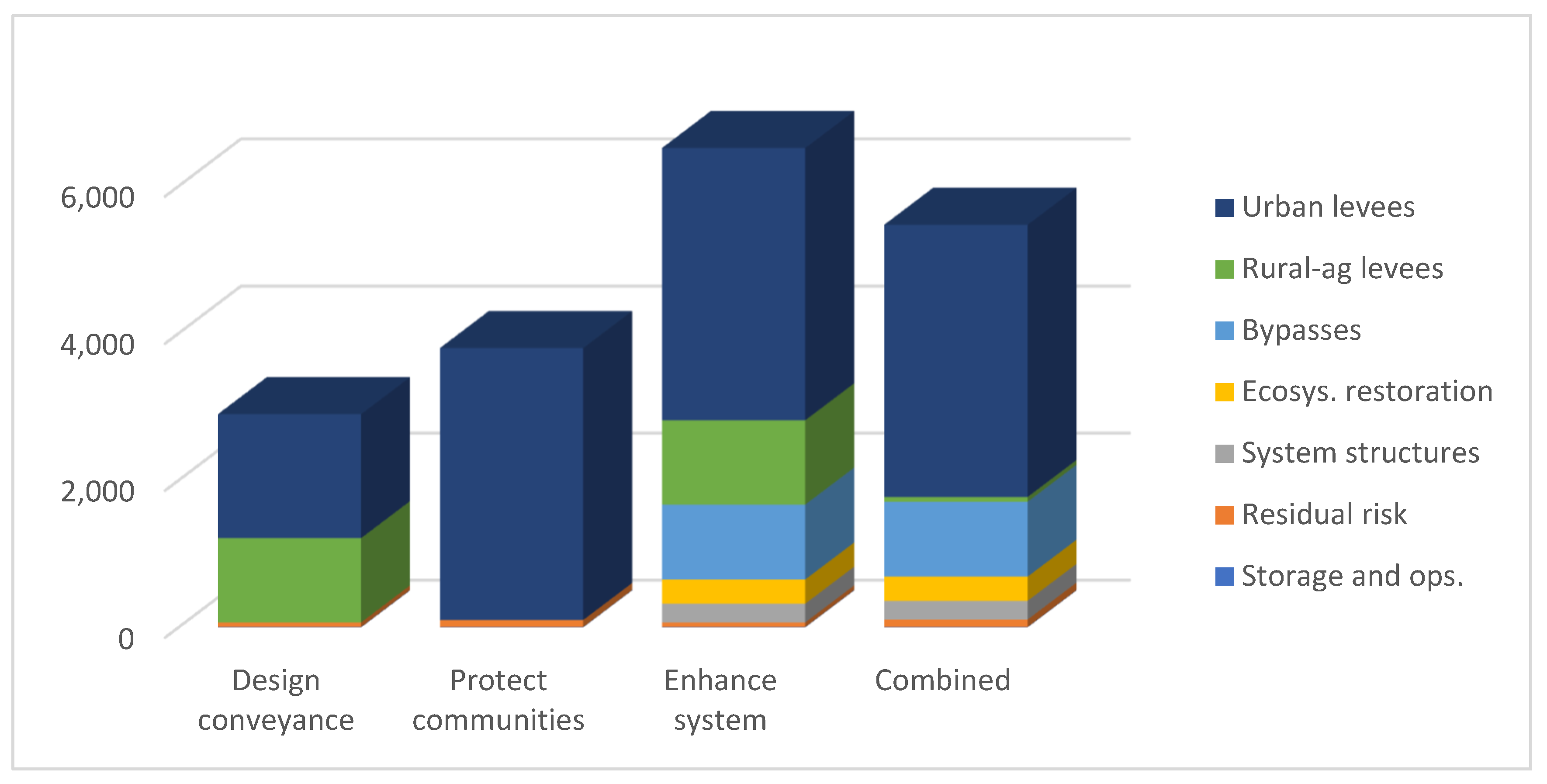
The plan developed for the CVFPP outlines three preliminary strategies for addressing the problems identified in the current SPFC as well as a fourth strategy that combines the strength of each of the preliminary strategies (Table 1). The Without Project baseline describes a continuation of existing conditions and projects currently authorized, e.g., current construction efforts to raise Folsom Dam. The Design Capacity (SPFC) strategy splits its budget between improvements to existing urban and rural SPFC levees so that they can convey their design flow (Figure 3). Alternatively, the strategy designed to Protect High Risk Communities (PHRC) focuses almost exclusively on urban levees in the Sacramento metro area. The third preliminary strategy took a more holistic approach to Enhance the Flood System Capacity (EFSC) and sought out opportunities to achieve multiple benefits throughout the basin. The EFSC strategy includes the levee improvements of the SPFC and PHRC strategies, but also a wide variety of additional management actions, including the inclusion of nature-based strategies, such as: Expansion of bypasses, conjunctive use, groundwater recharge, and ecosystem restoration (including floodplain restoration). A fourth strategy, the State Systemwide Investment Approach (SSIA) was then developed to combine the strengths of the three strategies above. The SSIA includes much of the same management actions as the EFSC, but reduces expenditures dedicated to rural levee improvements (Figure 3) (For a more detailed description of specific management actions included in each strategy, see the 2012 CVFPP [27]).
The CVFPP assessed each of the strategies, along with the baseline Without Project conditions, based on effectiveness in contributing to the CVFPP goals and other quantitative and qualitative performance measures, including: Level of flood protection, population with less than 100-year protection, EAD and reduction in EAD, capital costs, O&M requirements, opportunity for ecosystem restoration, opportunity for multi-benefit projects, ability to meet objectives in flood legislation, social sustainability, and climate change adaptability. The CVFPP analysis concluded that the Enhance System strategy, which includes the greatest extent of nature-based strategies, best meets CVFPP goals. However, it also requires the highest level of investment and significant institutional changes. Thus, CA-DWR adopted the Combined strategy to incorporate many of the beneficial features in the three preliminary strategies, including nature-based strategies such as widening channels to expand flood conveyance capacities and restoring floodplains, at a more reasonable cost and implementation time. This is the policy context in which the current effort attempted to introduce novel notions to planning in the face of climate change.
To add a climate change dimension to the CA-DWR analysis, we assessed the robustness of the management strategies in terms of their ability to meet the primary goal of flood risk reduction under a plausible range of future climates. Consistent with the CVFPP analysis and the U.S. Army Corps of Engineers (USACE) evaluation procedures for flood risk management plans [36,37], we based our climate risk metrics on EAD and reduction in EAD through management actions. This allows for consideration of climate change within the same decision context used in the CVFPP analysis, conveying information regarding future flood risks to decision makers using a familiar and well understood metric. While damages monetized through the EAD assessment only described a limited portion of flood risk, the methods presented herein could be applied to any of the performance measures included in the CVFPP, or others, e.g., population in the 100-year floodplain, loss of life, etc., or even metrics associated with the supplemental goals of the CVFPP. In addition to EAD, we also assessed the cost-effectiveness of the CVFPP strategies in terms of the benefit–cost ratio (BCR) over a wide range of plausible climate futures.
2.2. Sensitivity of the Current System to Flood Regime Changes
We assessed the current flood management system’s sensitivity to climate change by evaluating the relationship between flood risk, in terms of EAD, and changes in the hydrologic flood regime. EAD is a function of the probability of a flood event occurring multiplied by the damages expected to result from such an event [23]. Integrating flood damages over the probability of all possible flood events in a given year yields EAD (Equation (1)):
where, D(p) is the expected damages, D, in dollars, based on the probability of event (p).
Again, consistent with the CVFPP, our assessment only examined hydrologic changes and did not incorporate changes in the damage function, D(p), which could result, for example, from development and land use changes in the floodplain.
For flood risk management, the most important input to characterize hydrology is the probability distribution of annual peak flows, known as the flood-frequency curve [38]. In the U.S., flood forecasting by federal agencies follows the analysis techniques outlined in the Guidelines for Determining Flood Flow Frequency Bulletin 17B, commonly referred to as “Bulletin 17B”. Bulletin 17B recommends fitting a log-Pearson type III (LP3) distribution to observed annual maximum streamflow data using the method-of-moments to estimate the mean (μ), standard deviation (σ), and the skew coefficient (ϒ) [11]. In terms of potential changes to the flood frequency curve: Higher values of μ indicate larger expected values of flood magnitudes in any given year; higher values of σ indicate larger inter-annual variability in flood magnitude; and higher values of ϒ steepen the upper tail of the distribution, resulting in larger extreme events.
We based our initial flood frequency curve analysis on historic observations of daily streamflow gauge records collected on the American River at Fair Oaks gauge (USGS 11446500), located 11 km downstream of Folsom Dam, from 1905–2012. However, direct gauge data after the construction of Folsom Dam in 1955 represents regulated flow. Thus, we replaced the gauge data with estimated natural flows for the 1955–2012 period (Northwest River Forecast Center (NWRFC), unpublished data), which were calculated based on upstream gauges, storage volume, and release rates at Folsom. In this study, we assumed a skew parameter of zero for the LP3 distribution, which is a reasonable assumption for the historic period considering that the calculated station skew at Fair Oaks gauge is −0.035 with a standard deviation of 0.233 [39]. While this assumption may not hold into the future, limited historical records already result in unstable skew parameters [40], and projections of future skew are even more uncertain than mean and standard deviation. In addition, the zero-skew assumption simplifies the Bayesian analysis and does not detract from the methodological focus of the study.
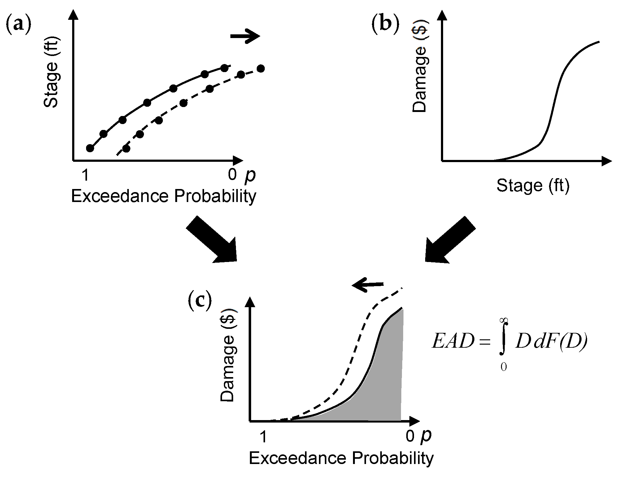
To assess the sensitivity of the current flood management system to different climates, we first developed a climate response function that describes the relationship between EAD and log-normal flood frequency curve parameter sets of μ and σ for the peak 3-day average discharge at Fair Oaks gauge. The mean daily unregulated inflow at Folsom Dam is one of the primary determinates of downstream flood risk, as there are no major inputs or outputs between Folsom and the City of Sacramento. We calculated EAD with a modeling suite that included the CVFPP using the USACE Hydrologic Engineering Center’s Flood Damage Assessment software (HEC-FDA) [27,33]. The HEC-FDA model uses stage-exceedance probability curves and damage-stage curves to estimate EAD (Figure 4). For the CVFPP, the stage-exceedance probability curves represent the downstream floodplain stage associated with flows entering Folsom reservoir, i.e., unmodified 99.9-, 10-, 4-, 2-, 1-, 0.5-, and 0.2-percent exceedance events flows at the Fair Oaks gauge (Figure 4a). Development of these stage-exceedance curves required the routing of flows through Folsom Reservoir and then to downstream regions using HEC Reservoir Simulation (RES-SIM) and HEC River Analysis System (RAS) models, respectively. Using in-channel stage and probability of levee failure curves, flood flows were then routed through a FLO-2D model to determine downstream floodplain stage. The damage associated with different floodplain stages (Figure 4b) considered:
- Residential, commercial, industrial, and governmental structure and contents damage;
- Agricultural/crop losses; and
Business production losses. See CVFPP 2012 [27] Attachment 8F for a full description of the Flood Damage Analysis and associated models.
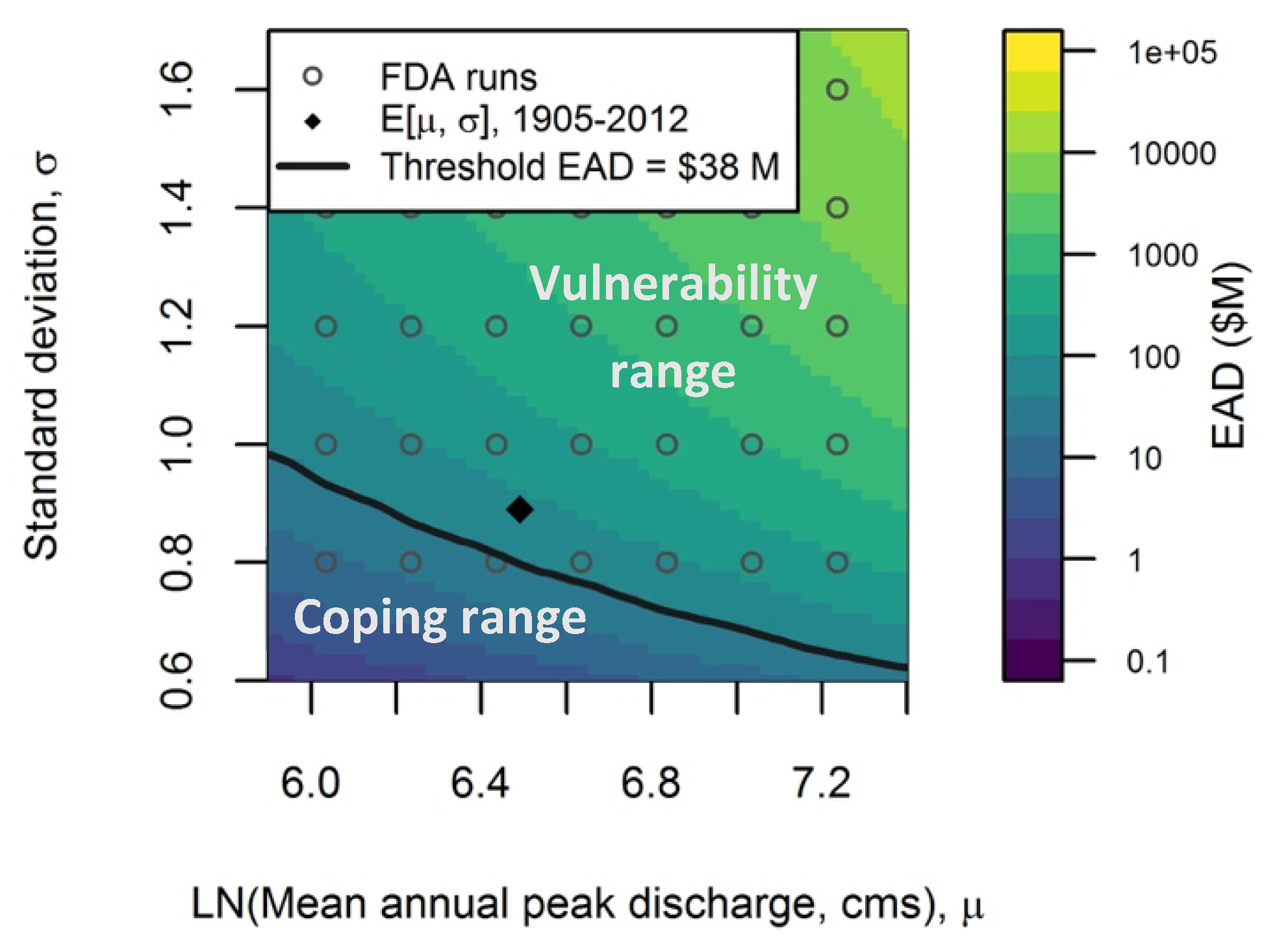
Using the HEC-FDA model, we assessed EAD across a gridded range of μ and σ parameter sets representing different flood frequency curves (Figure 5). For each parameter set, we calculated the probability of exceeding the river stage associated with the historic 99.9-, 10-, 4-, 2-, 1-, 0.5-, and 0.2 exceedance events (dotted line in Figure 4a) and combined this with the stage-damage curve (Figure 4b) to develop damage-exceedance plots (Figure 4c) and EAD values for each gridded parameter set (open circle locations in Figure 5). Due to the stepwise nature of the damage functions, where flooding and damages only occur after a certain flood magnitude, low (μ, σ) combinations produce EAD values of $0, or no damage. We concentrated on the portion of the EAD functions that produce damages, i.e., those with σ values of 0.8 and above. To assess how EAD responds to changes in the flood frequency curve, we developed a continuous climate response surface for the Without Project conditions by fitting a linear climate response function to the discrete flood frequency curve parameter sets (Equation (2)):
where, EAD is Expected annual damages ($); μ is the mean of the 3-day peak flow; σ is the standard deviation; and βi are regression coefficients.
We developed climate response surfaces using Equation (2) to examine the sensitivity of EAD to changes in μ and σ (shaded background in Figure 5).
2.3. Vulnerability of System to Flood Regime Changes
After developing the climate response surfaces, we identified the range of flood frequency regimes under which the system is vulnerable to exceeding an acceptable flood risk. We accepted a threshold for acceptable flood risk as the EAD ($38 million/year) under the Combined strategy that was selected as the CVFPP management strategy moving forward [27]. As such, the system was considered vulnerable when mean and standard deviation combinations yield EAD above the threshold of $38 million. We termed the region above the threshold the “vulnerability range” and below the threshold the “coping range” [41], and used historical gauge data to assess the extent to which the current system is vulnerable to exceeding the threshold EAD (Figure 5).
2.4. Plausible Range of Future Flood Regimes
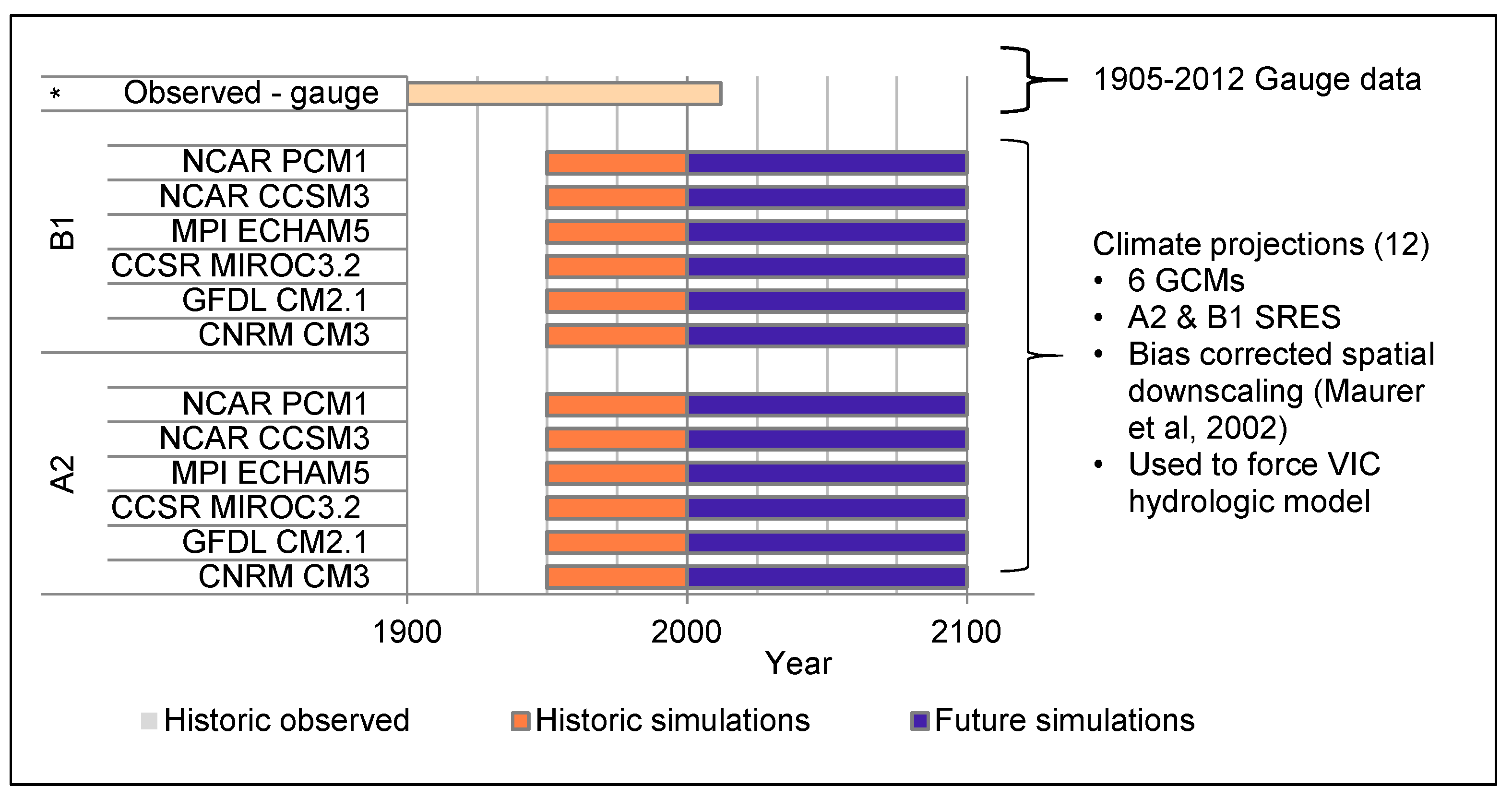
After assessing the sensitivity and vulnerability of the current system based on historic data, we then developed a plausible range of future flood regimes based on GCM simulations of future peak flow. We also used historic observations and historic GCM simulations to inform our confidence in the future simulations (Figure 6). In addition to the historical Fair Oaks gauge dataset, we assessed GCM-derived projections based on daily streamflow output from a Variable Infiltration Capacity (VIC) model of the Sacramento Basin, forced with Bias Corrected Spatially Downscaled (BCSD) output from two runs each of six GCMs [42,43]. We used streamflow simulations at a VIC index point on the American River at Folsom Dam, 11 km upstream of Fair Oaks and without significant inflow/outflow between the two locations. VIC output from 1950 to 1999 represent a forcing of the GCMs with observed atmospheric variables, downscaled and input into the hydrologic model. For the future time period (2000–2100), each GCM was forced with two climate change emissions scenarios (A2 and B1), totaling twelve sets of daily streamflow projections from 1950 to 2099.
We evaluated flood frequency parameters (μ, σ) for each of the historic and future flow datasets to both characterize plausible climate impacts on flood regimes and to qualitatively assess the reliability and uncertainty in the climate projections. This analysis included:
- Examining trends in flood frequency parameters based in the observed historic data (1905–2012);
- Comparing flood frequency parameters based on historic observations (1950–1999) and historic GCM simulations (1950–1999); and
- Comparing flood frequency parameters based on historic observations (1905–2012) and future GCM simulations (2000–2100).
In conducting the flood frequency analyses, we incorporated two major modifications to the methods outlined in Bulletin 17B. The first was the inclusion of future projections in addition to historic observations in the analysis. Secondly, we used Bayesian statistical techniques to develop plausible ranges of historic and future flood regime projections rather than Frequentist techniques. Bayes Theorem [44] treats the parameters of the probability distribution as variables themselves, which allowed for describing the parameters of fitted flood frequency curves (μ, σ) in terms of their own probabilistic distributions, conducive to developing our desired range of plausible impacts. For this analysis, using WinBUGS [45] we fit a log-normal Bayesian model with non-informative priors to the observed and simulated peak annual 3-day average flood discharge datasets. For each dataset, we used a Gibbs sampling Markov Chain Monte Carlo (MCMC) algorithm to produce 11,000 iterations, with the first 1000 used for burn in, to determine posterior intervals of the flood frequency parameters. To check convergence, we ensured that the Gelman-Rubin diagnostic results in values less than 1.05.
2.4.1. Trends in Mean and Standard Deviation of Flood Flows for the Historic Period (1905–2012)
We examined trends in the historical data, and projections based on those trends, to help establish a level of confidence in the future GCM-based projections. Studies examining climate trends often describe the factor of interest (e.g., precipitation, temperature, streamflow, etc.) in terms of the mean and variability over a period of time, typically 20 to 40-year intervals (e.g., [46,47]). As such, we fit log-normal flood frequency curves to moving 30-year time periods and examine trends in the fitted parameters over the historic period. Since flood frequency methods in Bulletin 17B generally only use the peak flow in any given year, the number of data points was low and equivalent to the number of years analyzed. The small sample size associated with extreme events made conclusive trend analysis difficult [48]. As a result, while we examined a 30-year moving average of the μ and σ of the peak discharge to investigate historical trends, results remain highly uncertain.
2.4.2. Comparison of Historic Observations and Historic GCM Simulations (1950–1999)
To assess the reliability of the GCM projections in projecting observed conditions, we compared the posterior intervals of the Bayesian flood frequency parameters (μ and σ) fit to the gauge observations and those fit to the GCM projections forced with observed historical emissions scenarios from 1950–1999.
2.4.3. Comparison of Historic Observations (1905–2012) and GCM Projections (2000–2099)
Lastly in developing the plausible impact range, for the historic observed and twelve future projected peak flow datasets (Figure 6), we generated 10,000 Markov chain samples of (μ, σ) combinations representing flood frequency curves. The resulting 120,000 parameter sets derived from the future GCM projections defined our plausible range of future flood regimes. We compared the posterior intervals of the parameter sets derived from future GCMs to those derived from the historic record to assess potential hydrologic responses to climate change.
2.5. Robustness of Current Systems and Management Strategies
In the last step of the bottom-up decision-making approach, we combined the vulnerability and impact assessment to determine the robustness of the current system and proposed management strategies. Consistent with Lempert, et al. [20] we defined robust strategies as those that perform reasonably well compared to the alternatives across a wide range of plausible scenarios. As an indicator of the robustness, we calculated the percentage of the draws from the posterior flood frequencies parameter sets below an established vulnerability threshold (Equation (3)):
A robustness value of one indicates that the full range of flood regimes lies below the threshold, and thus the system is not vulnerable to exceeding the decision threshold. On the other end of the spectrum, a robustness value of zero indicates that the system fails to meet the performance threshold under any of the plausible scenarios, making it extremely vulnerable to future conditions.
We used two different robustness thresholds, one a measure of flood risk (EAD) and the other a measure of cost-effectiveness (BCR). We assessed the robustness of the current system and management strategies in terms of the EAD threshold of $38 million, by first developing EAD response functions for each of the management strategies using the same methods described in Section 2.2. We then determined how many MCMC parameter sets lie above and below the threshold. In addition, we developed climate response surfaces of the BCR (Equation (4)) for each of the management strategies under different flood regimes, to assess their cost-effectiveness:
where BCR is the benefit–cost ratio ($/$), EADWO is the EAD under Without Project conditions, EADmanage is the EAD under one of the management strategies, r is the discount rate, t is life of the strategy, and cost is the cost of the management strategy.
Assessment of the BCR presented difficulties when trying to align the spatial extent of costs and benefits. We measured benefits in terms of EAD reduction within the American River Basin, however the cost estimates [27] included all projects located within the lower Sacramento region, of which the American River is a sub-basin. As such, the cost estimates included projects outside of the American basin, some of which would influence EAD within the American basin (e.g., expansion of Yolo Bypass) and some of which only produce benefits outside the American basin (e.g., mainstem levee improvements downstream of the confluence of the American). In addition, the projects included in the costs produce benefits outside of the American Basin, which are not included in the benefits calculation. To roughly address the incongruence with costs and benefits, similar to the EAD threshold, we set the BCR decision threshold to the BCR of the Combined strategy under historical flood conditions, namely 0.2 [27].
3. Results
We present the results of the bottom-up analysis by first discussing the sensitivity and vulnerability of the current system, based on historic data. We then present a range of plausible future climates and finally an assessment of the robustness of the current and possible future flood management strategies.
3.1. Sensitivity of Flood Risk (EAD) to Changes in Flood Frequency Regimes
The climate response equation produced a good fit (Table 3) to the gridded sets of (μ, σ), providing useful insight into the sensitivity of the current system to changes in the flood regime. The sensitivity of EAD to the flood frequency parameters is represented by β1 and β2 (Table 3). Small increases in the mean and standard deviation of peak annual floods yield large changes in EAD, indicating a high sensitivity to flood regime changes (Figure 5). For example, an increase in μ from 6.3 to 6.4 (540 to 600 m3/s, 11% increase) with σ = 0.9, yields a 27% increase in EAD from approximately $55M to $70M. EAD increases logarithmically from the lower left corner of the climate response surfaces to the upper right corner (Figure 5). We note that the linear model exhibits some heteroscedasticity, with larger residuals at high μ and σ. We discuss potential implications of this in Section 3.4.2 and Section 4.
3.2. Vulnerability above Threshold EAD
The Without Project system currently operates in the vulnerability range, with EAD above the threshold of $38M (Figure 5). A posterior median of μ and σ (6.49, 0.89) based on historic data from 1905–2012, yields an EAD of $79M, shown with the black diamond in Figure 5. In Section 3.4, we describe the results of combining the vulnerability assessment with the impact assessment to determine the robustness of each management strategy.
3.3. Plausible Range of Future Flood Impacts
The plausible range of future flood regimes developed using a Bayesian analysis of GCM simulations overlapped the range of historic hydrologic conditions, while extending into much higher ranges of μ and σ. The GCM and Bayesian-based range of future regimes was also in line with the increasing trends indicated by historic flood flow observations, as described subsequently.
3.3.1. Trends in Historical Gauge Data (1905–2012)
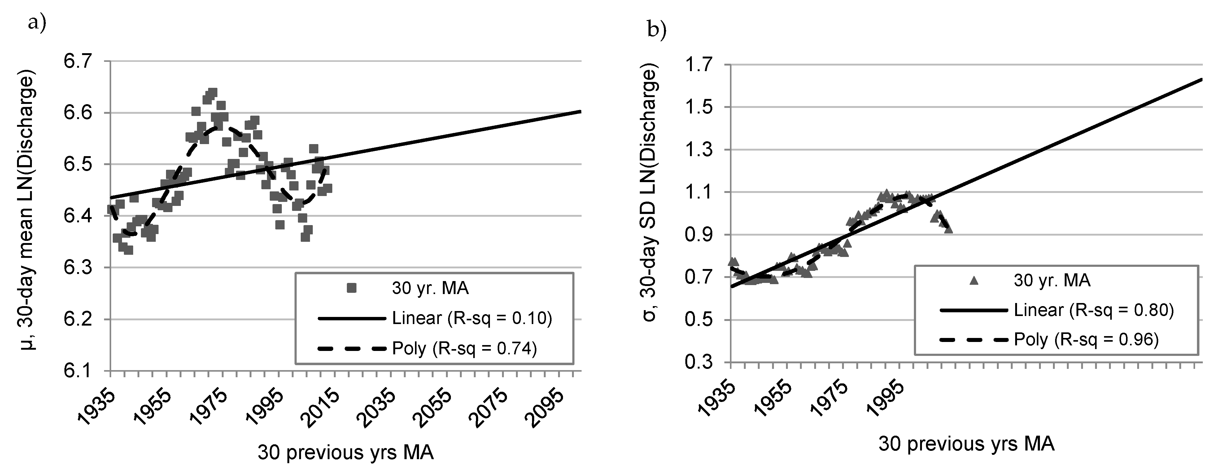
Calculating a simple 30-year moving μ and σ for the historic period reveals an increasing trend in the σ and a smaller increasing trend in μ (Figure 7). For the historic period (1905–2012), the 30-year mean of the LN-peak annual flood flow ranges from 6.33 to 6.64, and the standard deviation ranges from 0.68 to 1.10. Projecting the linear trend into 2050 indicates an E(μ) = 6.55 (1670 m3/s) and E(σ) = 1.32 (3630 m3/s). By 2100, and with less certainty, the linear trend indicates an E(μ) = 6.60 (2644 m3/s) and E(σ) = 1.60 (9134 m3/s). Furthermore, a short-term cyclic trend in the moving averages is apparent (Figure 7a) and described with good fit by fourth degree polynomial functions. This simple analysis demonstrates that the mean and standard deviation of the flood frequency parameters appear to exhibit short-term increasing and decreasing cycles with some evidence of increasing long-term trends, particularly for σ.
3.3.2. Comparison of Historic Observations and Historic GCM Simulations (1950–1999)
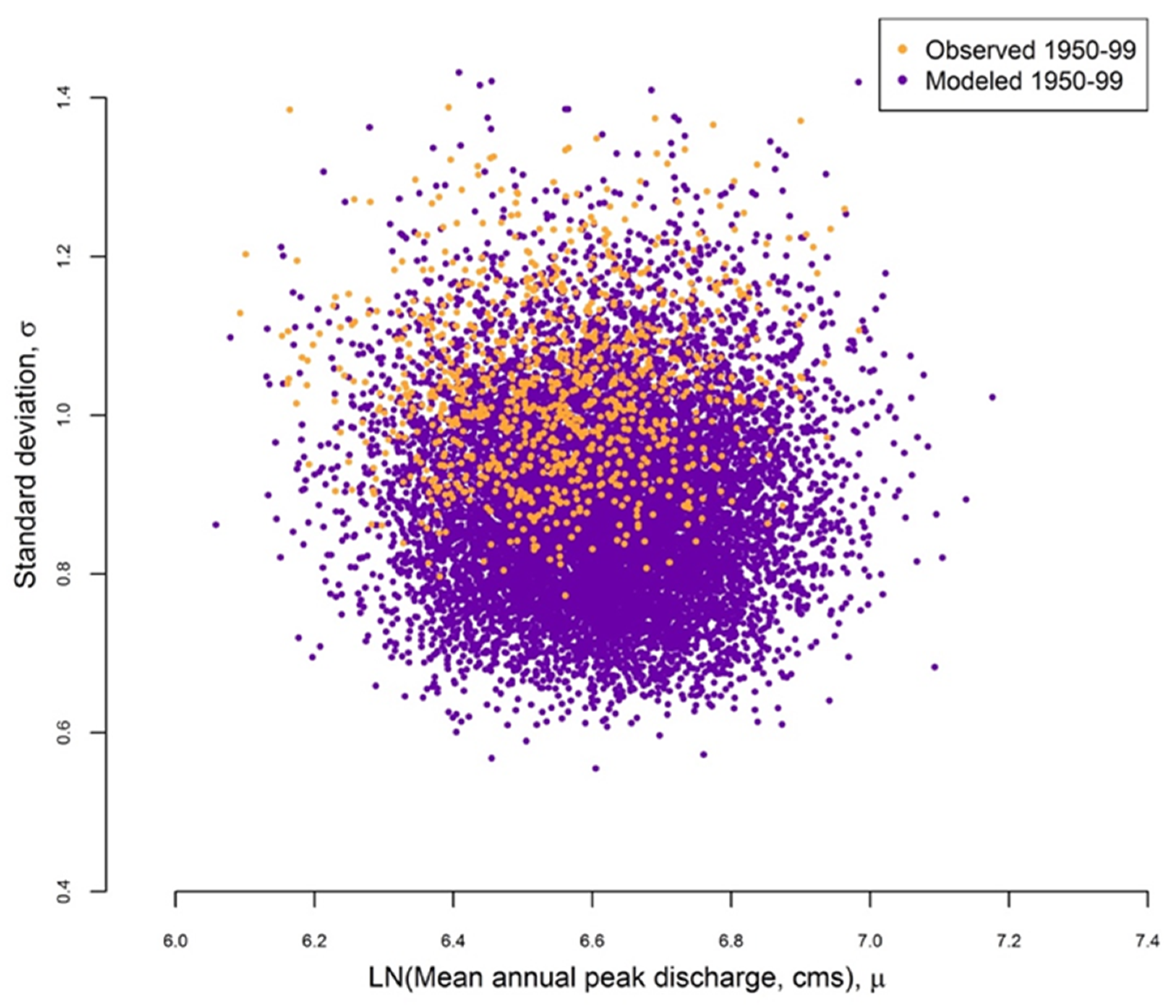
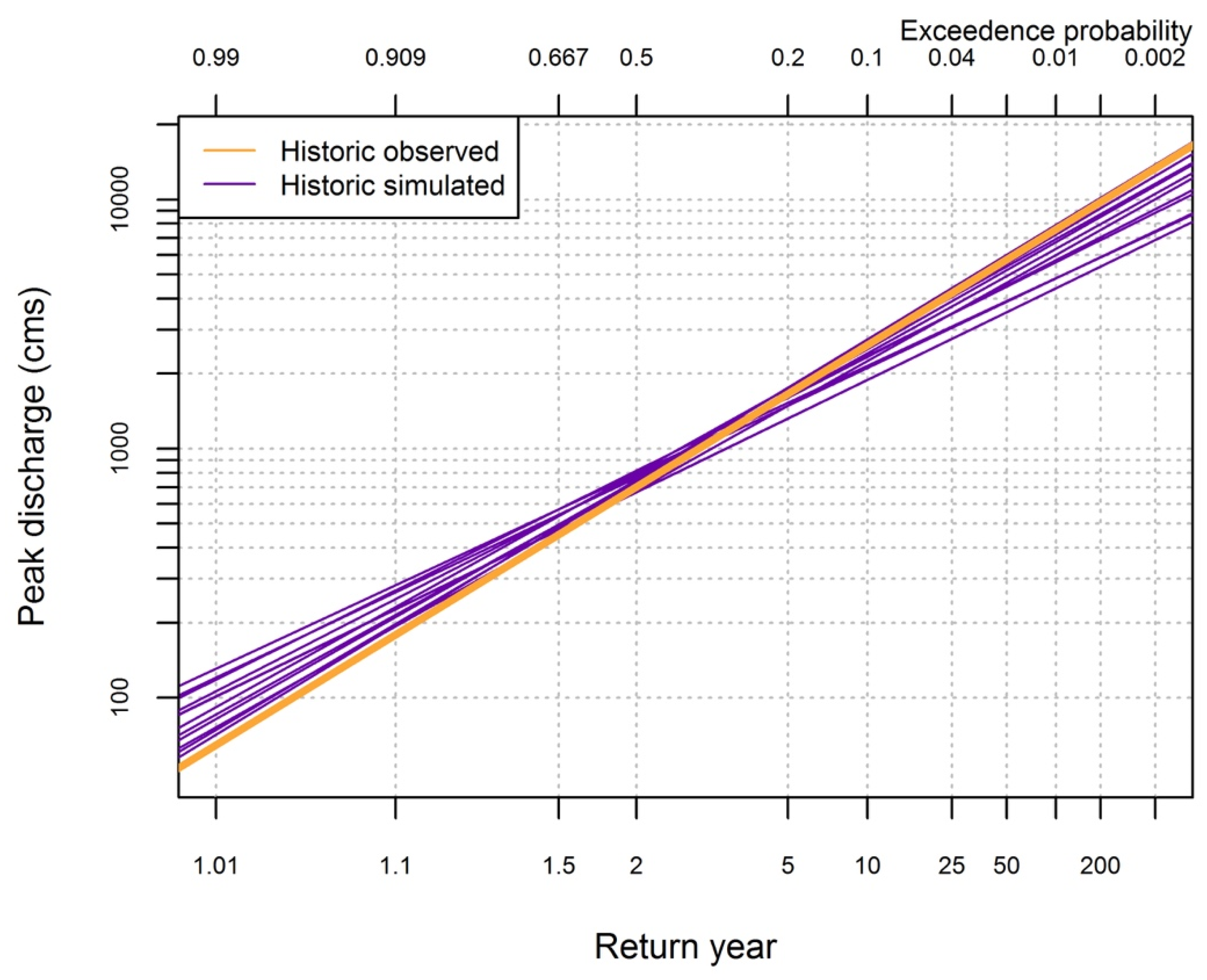
A comparison of the downscaled GCM output and the historic observed data from 1950–1999, illustrates the uncertainty in GCM projections for daily extreme precipitation, as other studies have found [42,43]. However, the GCMs more accurately estimate the historic mean (μ) of peak annual flood flows than the historic standard deviation (σ) of flood flows (Figure 8). These differences in posterior parameters produce substantially different flood frequency curves, particularly for estimations of more extreme events (e.g., 100-year, 200-year floods) (Figure 9). The parameter μ represents the 50% exceedance probability event, whereas σ determines the slope of the flood frequency curve (Figure 9). The lower σ values of the GCM simulations resulted in flood frequency curves with gentler slopes, leading to underestimations of extreme events compared to the curve fit to the historic gauge data. For example, based on the historic data, the expected magnitude of a 100-year flood is approximately 7500 m3/s, while the expected magnitude based on the GCMs ranges from 4400–7900 m3/s. The GCMs’ lack of skill in capturing the mean and variation in the historic data, even after bias correction, illustrates of the deep uncertainty associated with the downscaled model projections and the inability of a small set of GCM projections to reliably assess the full range of future flood risk. To capture some of this uncertainty, we present climate impact (Section 3.3.3) and robustness (Section 3.4) results in terms of the full distribution of flood frequency parameters, rather than only using the posterior median of the parameters.
3.3.3. Future Climate Impact Assessment
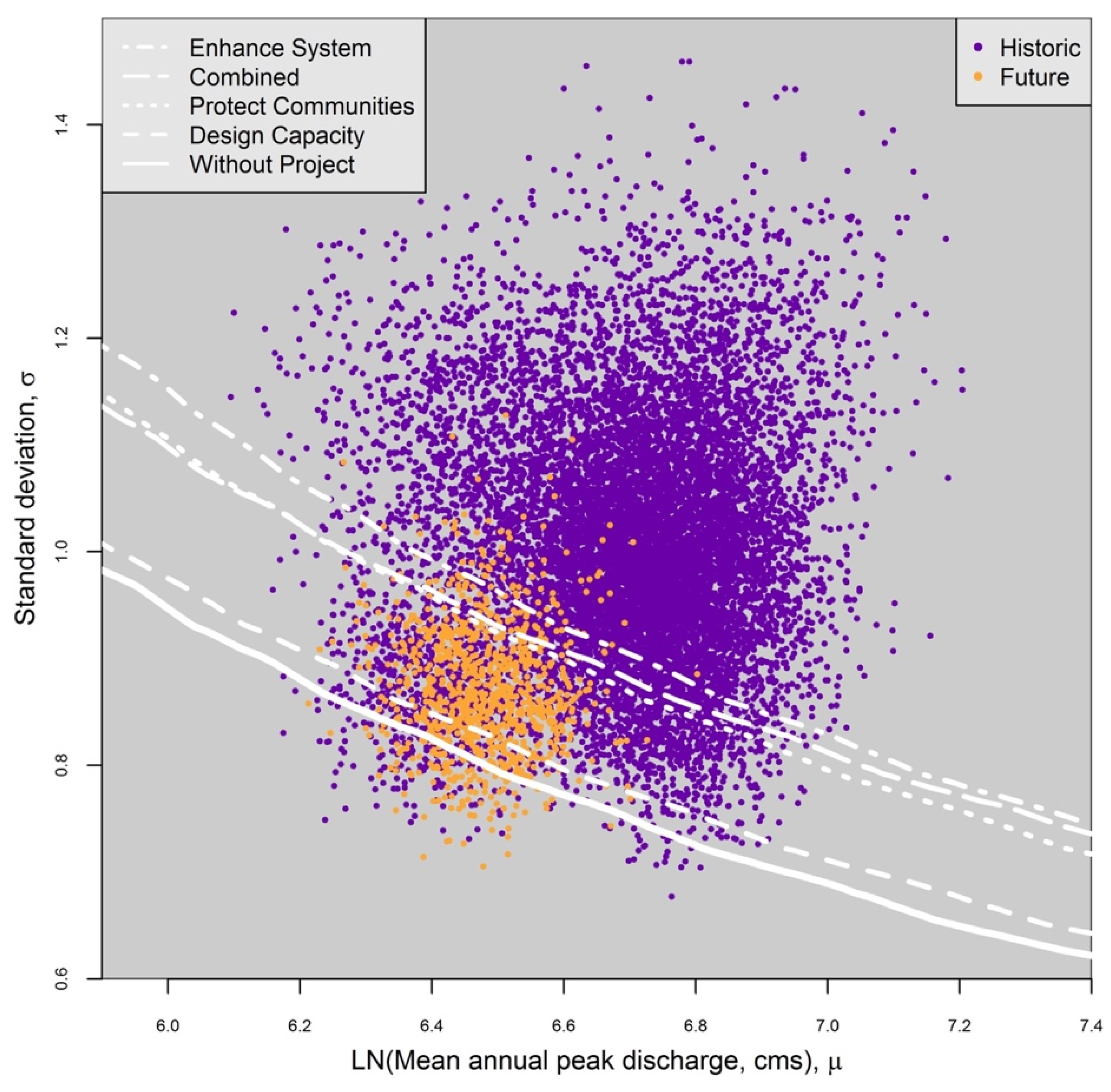
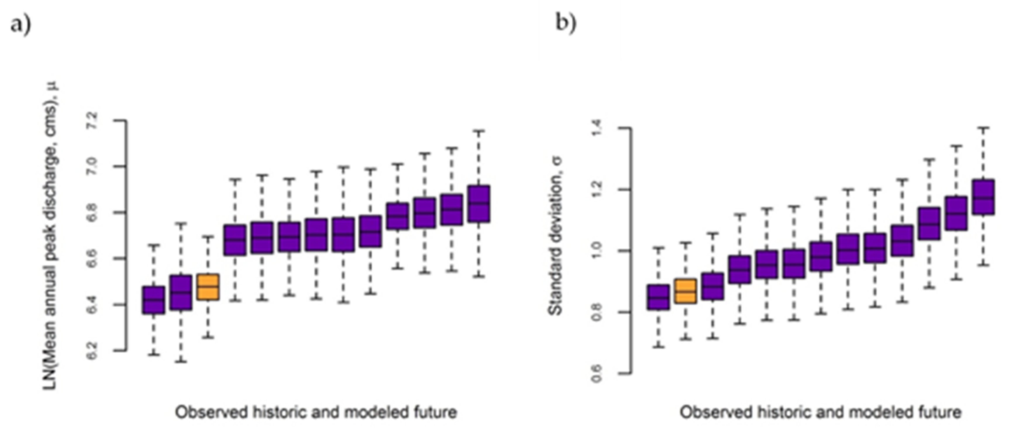
The plausible range of the flood frequency parameters developed from the posterior samples fitted with the GCM output, encapsulated the range of historic hydrologic conditions while extending into much higher ranges of μ and σ (Figure 10). The lower bound of the future plausible range for the mean and standard deviation projected with the GCMs resembles the lower bound of the parameter estimates based on the historical data (Figure 10). However, the upper bound on the plausible ranges developed from the GCMs extends far beyond the posterior samples based on the historical data. As such, the historic output occupies the lower left quadrant of the GCMs projections, the region of the lowest flood risk (Figure 10). Ten of the twelve GCMs project a larger posterior median μ for the future peak annual flood discharge than the historic peak (Figure 11a), and eleven of the twelve GCMs project a higher posterior median σ than under historical conditions (Figure 11b). These projected increases in μ and σ are consistent with the results identified previously in the historic data (Section 3.4.1).
3.4. Robustness of Current System and Management Strategies
We assessed robustness in terms of flood risk (EAD) and cost-effectiveness (BCR), which yielded related, but different results.
3.4.1. Robustness in Terms of Flood Risk, EAD
Under historic hydrologic conditions, the current Without Project system exhibits the lowest robustness in terms of EAD, though this is greatly improved under the proposed management strategies (Table 4). Eighty-two percent of the draws from the posterior distributions of the flood frequency parameters derived from the historic observations lie in the vulnerability range above the Without Project threshold (Figure 10). This indicates that the current system is predominantly operating outside of its coping range. However, each of the proposed management strategies would increase system robustness. Under the Enhance System strategy, 93% of the draws from the posterior distributions under historic hydrologic conditions lie below the EAD threshold (Table 4, Figure 10), making the strategy with the greatest focus on nature-based solutions, the most robust strategy. The Combined and Protect Communities strategies demonstrate very similar robustness, with overlapping contour EAD threshold lines (Figure 10). Lastly, the Design Capacity strategy exhibits the least robustness over the Without Project scenario.
While the management strategies perform well in terms of robustness based on historical conditions, the robustness of all of the strategies critically declines under the plausible range of future conditions. Under the future simulations and Without Project flood management, only 1% of the draws from the posterior distributions lie below the EAD threshold (Table 4, Figure 10). Although the most robust Enhance System strategy performs very well under historic conditions, under the future simulations only 22% of the draws from the future posterior distributions lie below the threshold.
3.4.2. Robustness in Terms of Cost-Effectiveness of Damage Reduction, BCR
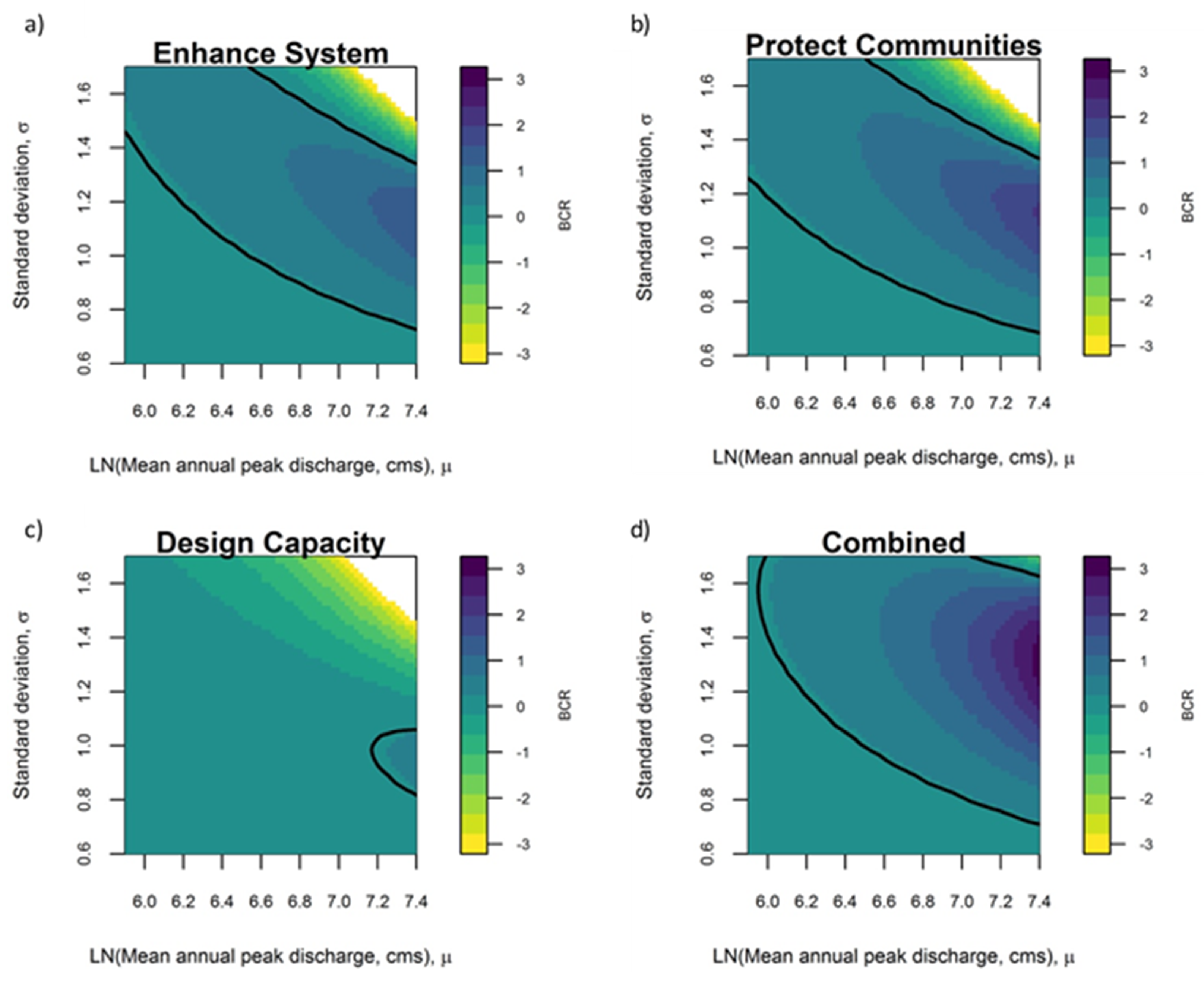
As μ and σ increase from historic conditions, the reduction in EAD and the BCR of each of the management strategies initially increases, but then begins to decrease at higher μ and σ (Figure 12). In contrast to the EAD robustness, the robustness of each of the management strategies relative to the BCR, increases under future conditions (Table 5). In other words, the cost-effectiveness of the management actions increases under higher μ, σ combinations and more extreme flood regimes. The Protect Communities exceeds the BCR threshold under the largest portion of plausible future conditions, while the Design Capacity strategy does not meet the threshold BCR under any of the historic or future scenarios. Furthermore, under the Design Capacity strategy, very high μ, σ combinations yield EAD that are actually higher than under the Without Project conditions. This also occurs to a lesser extent under the Enhance System strategy, leading to negative BCRs in the upper right-hand corner of Figure 12b,c. Importantly, we only consider benefits and costs associated with reductions in monetary flood damages, and do not account for other impacts that could significantly alter the BCR, particularly in regard to the three sub-goals of the CVFPP to improve operations and maintenance; promote ecosystem functions; improve institutional support; and promote multi-benefit projects.
4. Discussion
The potential for changes in flood regimes due to climate change, in combination with the deep limitations of climate projections, necessitates rethinking how we make flood risk management decisions. While bottom-up climate assessments hold promises as a new way to view water resources management under climate change, few studies have carried out a full bottom-up approach to flood risk management in practice. In addition, many options exist within the broadly outlined approaches in the literature [5,15,16,17,20] that need to be explored further. In developing a bottom-up climate assessment of flood risk for the American River flood management system, we identified several key ideas about both the bottom-up methodology and about flood risk within the American River system, with the goal of establishing a methodology that will aid water managers everywhere to better understand the hydrologic conditions that push a flood management system into a vulnerable state. We begin our discussion around the methodology employed, and then discuss the results for the American River basin in particular.
The methods used for the sensitivity and vulnerability assessment allow water managers to identify the hydrologic conditions that shift the system into a vulnerable state, using only the historic data and models currently available in the American River basin. Our method of fitting EAD response curves to a grid of flood frequency curve parameters (μ, σ) provides a computationally efficient method to assess the sensitivity of a system to a large range of potential flood regimes. However, this method does have limitations. Some accuracy is lost in fitting a linear model to a relatively small number of HEC-FDA runs, particularly at the lowest and highest range of μ, σ combinations. However, the R2 value for these equations fitted to the FDA model runs, range from 0.79 to 0.87, providing an adequate fit for a reconnaissance level pre-project planning analysis, such as presented in the 2012 CVFPP.
We used the EAD under the CVFPP strategy moving forward as a simple, justifiable method to determine the EAD vulnerability threshold, but many bottom-up approaches emphasize the importance of including stakeholders in process, particularly the vulnerability assessment [51,52,53]. Such a process might have revealed metrics of performance beyond EAD that could have been evaluated using the methodology developed through this research. Unfortunately, the time required to collaboratively establish acceptable risk thresholds is beyond the scope of our work. We acknowledge the lack of stakeholder participation as a shortcoming in our case study.
To capture some of the uncertainty associated with the future projections and incorporate it into the decision-making process, we used Bayesian techniques to develop a wide range of plausible flood frequency regimes characterized by their statistical parameters, μ and σ. Using draws from the posterior parameter sets in combination with the climate response surfaces enabled us to quickly calculate the EAD under thousands of plausible future flood regimes. The Bayesian analysis also lends itself to a variety of techniques to combine the historical and future data depending on its uncertainty and the decision at hand. For example, while we used non-informative priors throughout the study, it is possible to inform future flood frequency parameters with prior information based on the historical data or to weight GCMs based on their performance in projecting historic flood regimes, or other criteria. Determination of the plausible range of future scenarios would then incorporate, and place weight on, the historical record. In addition, rather than examining the 12 sets of future projections in isolation, we could use a hierarchical Bayesian model to combine the projections from different GCMs and emissions scenarios, and then examine the hyper-parameters that guide μi and σi, the posterior flood frequency parameters for each set of future projections. Furthermore, adding the skew parameter, ϒ, to the Bayesian analysis in order to fit LP3 distributions to the historic and future data, could improve the fit of the distribution, but it could also add more uncertainty with the additional parameter.
Assessing the proposed management strategies based on two different robustness parameters demonstrated how the climate response surfaces can be adjusted for different metrics, as well as the importance of examining all pertinent criteria for decision-making. Our assessment based on EAD demonstrated the extent to which the management strategies increase the robustness of the systems, but it only examines flood risk benefits without examining cost of the strategies. Adding costs into the analysis, as well as the net benefits over the life of the project, rather than average damages (EAD), provided an alternate perspective on the cost-effectiveness of the projects. Nonetheless, these two metrics only address the primary goal of the CVFPP, to reduce flood risk, and neglect to consider the three sub-goals, namely to improve operations and maintenance; promote ecosystem functions; improve institutional support; and promote multi-benefit projects. Similar climate response surfaces could be developed for metrics to assess the three sub-goals of the CVFPP.
Our case study demonstration of a bottom-up methodology also revealed interesting points regarding flood risk within the American River system and the robustness of proposed management actions. We found that the EAD of the American River flood management system is highly sensitive to small changes in the flood frequency parameters, which brings up two points of concern. First, real changes in the flood regime due to nonstationarity could result in very different damage scenarios for the basin. Secondly, considering the uncertainty associated with flood frequency parameters, even those calculated with observed gauge records, water managers must use caution in basing decisions on the median or mean EAD without considering the uncertainty of the calculation and sensitivity of EAD to the frequency parameters.
In terms of vulnerability, we found that the current system operates in a vulnerable state with a median EAD above the threshold EAD, as expected. The vulnerability of the flood management system to current conditions provided the impetus to invest in improving the system through the CVFPP management strategy.
To increase the utility of the vulnerability assessment, we used historic observed and future project hydrologic data to develop a plausible range of future flood regimes and establish our confidence in that range. Our results demonstrated poor skill in the ability of GCM model runs forced with observed parameters to capture the statistical parameters of the observed historic flood regime of the American River. It may be possible to improve the model skill by applying a bias correction aimed specifically at addressing the errors in projecting extreme precipitation events.
Some correlation was found between future model projections and trends in the historic data; however, trends based on the historic data exhibit a high degree of uncertainty due to the limited length of the gauge record. Further, we in no way demonstrate that the historic trend in increased flood regime intensity is linked to anthropogenic climatic changes. Nonetheless, both the future GCM projections and historic data trends indicate a similar increase in the flood frequency mean and standard deviation over time. These results are also in agreement with the physical science governing floods under climate change and direct output from the GCMs, which suggest warmer winters with more precipitation in the Sierra Nevada mountain range [2,54,55].
Our results also highlight differences in the robustness of different flood management strategies in the CVFPP, depending on whether robustness is measured in terms of flood risk (EAD) or cost-effectiveness (BCR). The Enhance System strategy, which included the greatest focus on nature-based strategies, provides the greatest robustness in terms of EAD, and is also the most expensive strategy. Taking project costs into consideration, the Protect Communities strategy exhibits the greatest robustness in terms its ability to maintain a BCR above the threshold for the largest portion of the plausible future range. The Combined strategy exhibited the second highest robustness indicator values for both metrics, and is also the second most expensive strategy.
The results of the robustness assessment lead to important planning considerations. While all of the proposed strategies offer substantial gains in EAD robustness under historic hydrological conditions, the robustness drops drastically when considering the plausible range of future climate impacts. As such, decision-making processes that neglect to consider future impacts run the danger of implementing strategies that do not reduce risk as much as expected. Alternatively, the cost-effectiveness of the management strategies initially increases in value under more extreme flood conditions. As such, some management strategies may become more financially appealing when future hydrologic conditions are taken into consideration.
While our results describe the conditions that may favor one strategy over another, the uncertainty associated with climate change and the wide plausible range of future conditions say little to nothing about which conditions we expect to occur in the future. However, over the course of the long implementation time (15–40 years) for the CVFPP strategies, advances in modeling, data, and analysis methods may allow us to track changes in observed flood frequency, narrow the plausible range of future conditions by decreasing uncertainty, and/or better describe uncertainty and associate probabilities with future conditions. As we gain such knowledge, we can adapt our decision-making process and management strategies to the expected future conditions.
5. Conclusions
The bottom-up methodology addresses arguably the two largest challenges facing future flood management, namely, the lack of: (1) Climate projections that can reliably represent historic conditions at the temporal and spatial resolution required for flood frequency analysis, and (2) methods to tailor climate projections into information useful to flood managers. Beginning the climate assessment process from the bottom-up enabled us to describe the sensitivity and vulnerability of the system to changes in flood regime, using only historic data. The climate response surfaces provide flood mangers with a visual representation of the sensitivity and vulnerability of the system. On their own, these response surfaces can be used to assess whether the current system is operating above or below vulnerability thresholds, how flood risk might change under different flood regimes, as well as how different management strategies might affect system vulnerabilities. Furthermore, by combining the response surfaces with future climate projections, we can assess the robustness of the current system and management strategies in terms of their ability to meet a performance threshold under a large portion of the plausible range of future conditions.
Our case study of the CVFPP in the American River basin provided an opportunity to demonstrate the utility of bottom-up methods, while yielding insight into the sensitivity, vulnerability, and robustness of the American River basin and management strategies proposed in the CVFPP. Our analysis intentionally limited data sources and models to those already included in the 2012 CVFPP, making it relatively easy to expand to the larger Central Valley planning region and/or narrow for more detailed robustness assessments of the refined set of management actions included in the Updated 2017 CVFPP [56]. As the planning and implementation process for the CVFPP moves forward and more money is at stake, the importance of considering climate impacts increases, along with the consequences of not considering climate impacts.
While bottom-up approaches hold promise for future water resources decision-making, very few applications exist in practice and many questions remain regarding the specific methods to use. This leads the way for many potential avenues of future work related specifically to this study and bottom-up climate assessment more generally. In relation to climate risk assessment for the CVFPP, we recommend further work to: (a) Include public participation in identifying threshold metrics and levels; (b) include other metrics besides those focused on EAD (i.e., those that address the sub-goals of the CVFPP); (c) consider different methods to combine historic and future data (i.e., informative priors of future projections based on historical data); and (d) consider other sources of uncertainty and nonstationarity (e.g., population growth and land change). More generally, the field of climate adaptation could benefit tremendously from more on-the-ground examples of climate risk assessment and adaptation planning.
Author Contributions
K.D. conceived and designed the study; A.G. advised and helped design the Bayesian statistical analysis; D.P. advised and provided strategic input on the developed bottom-up approach; K.D. led authorship of this paper, with invaluable contributions from D.P. and A.G. All authors have read and agreed to the published version of the manuscript.
Funding
This research was funded by the U.S. National Science Foundation under grant no. 0846360.
Acknowledgments
Thank you to Desiree Tullos for supervising the PhD research that contributed to this article.
Conflicts of Interest
The authors declare no conflict of interest.
References
- Hamlet, A.F.; Lettenmaier, D.P. Effects of 20th century warming and climate variability on flood risk in the western U.S. Water Resour. Res. 2007, 43, 17. [Google Scholar] [CrossRef]
- Das, T.; Dettinger, M.; Cayan, D.; Hidalgo, H. Potential increase in floods in California’s Sierra Nevada under future climate projections. Clim. Chang. 2011, 109, 71–94. [Google Scholar] [CrossRef]
- Willis, A.D.; Lund, J.R.; Townsley, E.S.; Faber, B.A. Climate change and flood operations in the Sacramento basin, California. San Franc. Estuary Watershed Sci. 2011, 9, 2. [Google Scholar] [CrossRef] [Green Version]
- Mote, P.; Brekke, L.; Duffy, P.B.; Maurer, E. Guidelines for constructing climate scenarios. Eos Trans. Am. Geophys. Union 2011, 92, 257–258. [Google Scholar] [CrossRef]
- Brown, C.; Wilby, R.L. An alternate approach to assessing climate risks. Eos Trans. Am. Geophys. Union 2012, 93, 401–402. [Google Scholar] [CrossRef]
- Prudhomme, C.; Reynard, N.; Crooks, S. Downscaling of global climate models for flood frequency analysis: Where are we now? Hydrol. Process. 2002, 16, 1137–1150. [Google Scholar] [CrossRef]
- Hallegatte, S. Strategies to adapt to an uncertain climate change. Glob. Environ. Chang. 2009, 19, 240–247. [Google Scholar] [CrossRef]
- Wilby, R.L.; Dessai, S. Robust adaptation to climate change. Weather 2010, 65, 180–185. [Google Scholar] [CrossRef] [Green Version]
- Roe, G.H.; Baker, M.B. Why is climate sensitivity so unpredictable? Science 2007, 318, 629–632. [Google Scholar] [CrossRef] [Green Version]
- Knutti, R.; Sedláček, J. Robustness and uncertainties in the new CMIP5 climate model projections. Nat. Clim. Chang. 2013, 3, 369–373. [Google Scholar] [CrossRef]
- US Water Resources Council. US Water Resources Council Guidelines for Determining Flood Flow Frequency; US Water Resources Council: Washington, DC, USA, 1982.
- Xu, C. From GCMs to river flow: A review of downscaling methods and hydrologic modelling approaches. Prog. Phys. Geogr. 1999, 23, 229–249. [Google Scholar] [CrossRef]
- Fowler, H.J.; Blenkinsop, S.; Tebaldi, C. Linking climate change modelling to impacts studies: Recent advances in downscaling techniques for hydrological modelling. Int. J. Climatol. 2007, 27, 1547–1578. [Google Scholar] [CrossRef]
- Laprise, R.; De Elia, R.; Caya, D.; Biner, S.; Lucas-Picher, P.; Diaconescu, E.; Leduc, M.; Alexandru, A.; Separovic, L. Challenging some tenets of regional climate modelling. Meteorol. Atmos. Phys. 2008, 100, 3–22. [Google Scholar] [CrossRef]
- Prudhomme, C.; Wilby, R.L.; Crooks, S.; Kay, A.L.; Reynard, N.S. Scenario-neutral approach to climate change impact studies: Application to flood risk. J. Hydrol. 2010, 390, 198–209. [Google Scholar] [CrossRef] [Green Version]
- Brown, C.; Ghile, Y.; Laverty, M.; Li, K. Decision scaling: Linking bottom-up vulnerability analysis with climate projections in the water sector. Water Resour. Res. 2012, 48, 9537. [Google Scholar] [CrossRef]
- Jeuken, A.; Mendoza, G.; Matthews, J.; Ray, P.; Haasnoot, M.; Gilroy, K.; Olsen, R.; Kucharski, J.; Stakhiv, G.; Cushing, J.; et al. Climate Risk Informed Decision Analysis (CRIDA): A Novel Practical Guidance for Climate Resilient Investments and Planning; UNESCO International Center for Integrated Water Resources Management. 2016, Volume 18. Available online: https://unesdoc.unesco.org/ark:/48223/pf0000265895 (accessed on 21 March 2020).
- Gilroy, K.; Mens, M.; Haasnoot, M.; Jeuken, A. Climate Risk Informed Decision Analysis: A Hypothetical Application to the Waas Region. In Proceedings of the EGU General Assembly Conference Abstracts, Vienna, Austria, 12–22 April 2016; Volume 18. [Google Scholar]
- Hallegatte, S.; Shah, A.; Brown, C.; Lempert, R.; Gill, S. Investment Decision Making Under Deep Uncertainty—Application to Climate Change; Social Science Research Network: Rochester, NY, USA, 2012. [Google Scholar]
- Lempert, R.J.; Bankes, S.C.; Popper, S.W. Shaping the Next One Hundred Years: New Methods for Quantitative, Long-Term Policy Analysis; RAND Corporation: Santa Monica, CA, USA, 2003; ISBN 0-8330-3275-5. [Google Scholar]
- Johnson, T.E.; Weaver, C.P. A Framework for assessing climate change impacts on water and watershed systems. Environ. Manag. 2009, 43, 118–134. [Google Scholar] [CrossRef]
- Brown, C.; Werick, W.; Leger, W.; Fay, D. A decision-analytic approach to managing climate risks: Application to the upper great lakes. JAWRA J. Am. Water Resour. Assoc. 2011, 47, 524–534. [Google Scholar] [CrossRef]
- National Research Council (NRC), Committee on Risk-Based Analyses for Fio, Water Science and Technology Board. Risk Analysis and Uncertainty in Flood Damage Reduction Studies; The National Academies Press: Washington, DC, USA, 2000; ISBN 0-309-07136-4.
- Garcia, L.E.; Matthews, J.H.; Rodriguez, D.J.; Wijnen, M.; DiFrancesco, K.N.; Ray, P. Beyond Downscaling—A Bottom-up Approach to Climate Adaptation for Water Resources Management; World Bank Group: Washington, DC, USA, 2014. [Google Scholar]
- Frederick, K.D.; Major, D.C.; Stakhiv, E.Z. Water resources planning principles and evaluation criteria for climate change: Summary and conclusions. Clim. Chang. 1997, 37, 291–313. [Google Scholar] [CrossRef]
- Dessai, S.; Hulme, M. Assessing the robustness of adaptation decisions to climate change uncertainties: A case study on water resources management in the East of England. Glob. Environ. Chang. 2007, 17, 59–72. [Google Scholar] [CrossRef]
- California Department of Water Resources (CA-DWR). 2012 Central Valley Flood Protection Plan; CA-DWR: Sacramento, CA, USA, 2012.
- Dettinger, M.D.; Cayan, D.R.; Meyer, M.K.; Jeton, A.E. Simulated hydrologic responses to climate variations and change in the Merced, Carson, and American River Basins, Sierra Nevada, California, 1900–2099. Clim. Chang. 2004, 62, 283–317. [Google Scholar] [CrossRef]
- Dettinger, M.D.; Ralph, F.M.; Das, T.; Neiman, P.J.; Cayan, D.R. Atmospheric rivers, floods and the water resources of California. Water 2011, 3, 445–478. [Google Scholar] [CrossRef]
- Kelley, R.L. Battling the Inland Sea: Floods, Public Policy, and the Sacramento Valley; University of California Press: Berkeley, CA, USA, 1989. [Google Scholar]
- California Department of Water Resources (CA-DWR). State Plan of Flood Control Descriptive Document; CA-DWR: Sacramento, CA, USA, 2010.
- California Department of Water Resources (CA-DWR). Central Valley Flood Protection Plan Regional Conditions Report; CA-DWR: Sacramento, CA, USA, 2010.
- United States Army Corps of Engineers (USACE). Sacramento and San Joaquin River Basins Comprehensive Study 2002; USACE: Washington, DC, USA, 2002.
- Ferreira, J.; California Department of Water Resources (CA-DWR). A Preliminary Study of Flood Control Alternatives on the Lower American River; State of California, the Resources Agency, Department of Water Resources, Central District: Sacramento, CA, USA, 1982.
- Platt, R.H. Flood Risk Management and the American River Basin: An Evaluation; National Academies Press: Cambridge, MA, USA, 1995; ISBN 978-0-309-05334-1. [Google Scholar]
- United States Army Corps of Engineers (USACE). Risk-Based Analysis for Damage Reduction Studies; USACE: Washington, DC, USA, 1996.
- United States Army Corps of Engineers (USACE). Regulation No. 1105-2-101; USACE: Washington, DC, USA, 2006.
- Faber, B.A. Current methods for hydrologic frequency analysis. In Proceedings of the Workshop on Nonstationarity, Hydrologic Frequency Analysis, and Water Management, Boulder, CO, USA, 13–15 January 2010. [Google Scholar]
- Parrett, C.; Veilleux, A.; Stedinger, J.R.; Barth, N.A.; Knifong, D.L.; Ferris, J.C. Regional Skew for California, and Flood Frequency for Selected Sites in the Sacramento-San Joaquin River Basin, Based on Data through Water Year 2006; U.S. Geological Survey: Reston, VA, USA, 2011.
- Griffis, V.W.; Stedinger, J.R. Incorporating climate change and variability into Bulletin 17B LP3 model. In Proceedings of the World Environmental and Water Resources Congress, Tampa, FL, USA, 15–19 May 2007; pp. 1–8. [Google Scholar]
- Smit, B.; Wandel, J. Adaptation, adaptive capacity and vulnerability. Glob. Environ. Chang. 2006, 16, 282–292. [Google Scholar] [CrossRef]
- Maurer, E.P.; Hidalgo, H.G. Utility of daily vs. monthly large-scale climate data: An intercomparison of two statistical downscaling methods. Hydrol. Earth Syst. Sci. 2008, 12, 551–563. [Google Scholar] [CrossRef] [Green Version]
- Maurer, E.P.; Hidalgo, H.G.; Das, T.; Dettinger, M.D.; Cayan, D.R. The utility of daily large-scale climate data in the assessment of climate change impacts on daily streamflow in California. Hydrol. Earth Syst. Sci. 2010, 14, 1125–1138. [Google Scholar] [CrossRef] [Green Version]
- Bayes, M.; Price, M. An Essay towards solving a problem in the doctrine of chances. By the Late Rev. Mr. Bayes, F.R.S. Communicated by Mr. Price, in a Letter to John Canton, A.M.F.R.S. Philos. Trans. 1763, 53, 370–418. [Google Scholar]
- Lunn, D.J.; Thomas, A.; Best, N.; Spiegelhalter, D. WinBUGS-a Bayesian modelling framework: Concepts, structure, and extensibility. Stat. Comput. 2009, 10, 325–337. [Google Scholar] [CrossRef]
- Bengtsson, L.; Hagemann, S.; Hodges, K.I. Can climate trends be calculated from reanalysis data? J. Geophys. Res. Atmos. 2004, 109. [Google Scholar] [CrossRef] [Green Version]
- Lins, H.F.; Slack, J.R. Seasonal and regional characteristics of US streamflow trends in the United States from 1940 to 1999. Phys. Geogr. 2005, 26, 489–501. [Google Scholar] [CrossRef]
- Easterling, D.R.; Evans, J.L.; Groisman, P.Y.; Karl, T.R.; Kunkel, K.E.; Ambenje, P. Observed variability and trends in extreme climate events: A brief review *. Bull. Am. Meteorol. Soc. 2000, 81, 417–425. [Google Scholar] [CrossRef] [Green Version]
- US Federal Emergency Management Agency (FEMA). Appendix B. Understanding the FEMA Benefit-Cost Analysis Process. In Engineering Principles and Practices for Retrofitting Flood-Prone Residential Structures; FEMA: Jessup, MD, USA, 2001. [Google Scholar]
- California Department of Water Resources (CA-DWR). Climate Change Work Group Meeting #2 Minutes 2009; CA-DWR: Sacramento, CA, USA, 2009.
- Purkey, D.R.; Escobar Arias, M.I.; Mehta, V.K.; Forni, L.; Depsky, N.J.; Yates, D.N.; Stevenson, W.N. A philosophical justification for a novel analysis-supported, stakeholder-driven participatory process for water resources planning and decision making. Water 2018, 10, 1009. [Google Scholar] [CrossRef] [Green Version]
- Kloprogge, P.; Van Der Sluijs, J.P. The inclusion of stakeholder knowledge and perspectives in integrated assessment of climate change. Clim. Chang. 2006, 75, 359–389. [Google Scholar] [CrossRef]
- Few, R.; Brown, K.; Tompkins, E.L. Public participation and climate change adaptation: Avoiding the illusion of inclusion. Clim. Policy 2007, 7, 46–59. [Google Scholar] [CrossRef]
- Stocker, T.F.; Dahe, Q.; Plattner, G.-K. Climate Change 2013: The Physical Science Basis. Working Group I Contribution to the Fifth Assessment Report of the Intergovernmental Panel on Climate Change; Summary for Policymakers; Cambridge University Press: New York, NY, USA, 2013. [Google Scholar]
- Pachauri, R.K.; Allen, M.R.; Barros, V.R.; Broome, J.; Cramer, W.; Christ, R.; Church, J.A.; Clarke, L.; Dahe, Q.; Dasgupta, P.; et al. Climate Change 2014: Synthesis Report. Contribution of Working Groups I, II and III to the Fifth Assessment Report of the Intergovernmental Panel on Climate Change; Cambridge University Press: New York, NY, USA, 2014. [Google Scholar]
- CA-DWR (California Department of Water Resources). Central Valley Flood Protection Plan 2017 Update; CA-DWR: Sacramento, CA, USA, 2017.
Figure 1.
Map of the American River Basin, CA showing major State Plan for Flood Control (SPFC) project works.
Figure 1.
Map of the American River Basin, CA showing major State Plan for Flood Control (SPFC) project works.

Figure 2.
Daily hydrograph at Fair Oaks USGS gauge on the American River, CA.

Figure 3.
Expenditure on the components of each management strategy assessed in the CVFPP.

Figure 4.
Basis of the Expected Annual Damages (EAD) computation used in CVFPP Hydrologic Engineering Center’s Flood Damage Assessment software (HEC-FDA) model (modified from [27]): (a) Stage-exceedance curves, where the solid line indicates the stage-exceedance curve calculated in HEC-FDA from the 99.9-, 10-, 4-, 2-, 1-, 0.5-, and 0.2-percent exceedance events calculated using historical gauge data (points). The dashed lines and points indicate how the stage-probability curves were shifted to assess the sensitivity of EAD to different climates; (b) Stage-damage curve, where the solid line indicates the curve calculated in HEC-FDA from discrete exceedance events calculated using historical gauge data; (c) Damage-exceedance curves calculated in FDA by combining (a,b).

Figure 5.
Gridded FDA model runs (open circles) used in the regression model to develop the flood risk response surface, LN(EAD) = ƒ(µ, σ), under Without Project conditions (shaded background). The black diamond indicates the EAD based on historic data from 1905–2012. The system is vulnerable to flood regimes above the white threshold line where EAD = $38M.

Figure 6.
Observed and modeled daily streamflow used for historic (orange) and future (indigo) flood frequency analysis on the American River at Folsom.
Figure 6.
Observed and modeled daily streamflow used for historic (orange) and future (indigo) flood frequency analysis on the American River at Folsom.

Figure 7.
Expected value of 30-year (a) average (μ) and (b) standard deviation (σ) of LN-historic observed 3-day average peak annual flows. The solid lines represent long term linear trends fit to the moving average (MA), with fourth degree polynomial trends, displayed with the dashed lines.
Figure 7.
Expected value of 30-year (a) average (μ) and (b) standard deviation (σ) of LN-historic observed 3-day average peak annual flows. The solid lines represent long term linear trends fit to the moving average (MA), with fourth degree polynomial trends, displayed with the dashed lines.

Figure 8.
Posterior distribution draws for the observed historic data (1950–1999, orange circles) and each of the GCMs forced with historic data (1950–1999, purple circles).
Figure 8.
Posterior distribution draws for the observed historic data (1950–1999, orange circles) and each of the GCMs forced with historic data (1950–1999, purple circles).

Figure 9.
Expected posterior flood frequency curves derived from observed streamflow data (orange) and GCMs forced with observed parameters from 1950–1999 (purple).
Figure 9.
Expected posterior flood frequency curves derived from observed streamflow data (orange) and GCMs forced with observed parameters from 1950–1999 (purple).

Figure 10.
Posterior distribution draws for the historic data (1905–2012, orange circles) and each of the GCMs (2000–2099, purple circles). The contour lines represent the EAD threshold under Without Project conditions and the four management strategies outlined in the 2012 CVFPP. The percentage of posterior distribution draws below the threshold represents the coping range for both historic and future conditions, while the system remains vulnerable to conditions above the threshold lines.

Figure 11.
Posterior interval boxplots of: (a) Mean peak annual flow, μ, and (b) standard deviation, σ, of peak annual flow for observed streamflow data from 1905–2012 (orange box) and GCMs forced with future emissions scenarios (purple boxes) from 2000–2099. The whiskers signify the 95% posterior interval, with quartiles around the median value (black line) indicated with the boxes.

Figure 12.
Benefit–cost ratio (BCR) response surfaces for each of the management strategies: (a) Design capacity, (b) protect communities, (c) enhance system, (d) combined. The strategy exceeds the cost-effectiveness threshold for flood regimes between the black threshold lines where BCR = 0.2. BCR below −3 are displayed in white.


Table 1.
Overview of Central Valley Flood Protection Plan (CVFPP) management strategies.
| Short Name | CVFPP Name [27] | Strategy Description and Spatial Focus [27] | Inclusion of Nature-Based Strategies |
|---|---|---|---|
| Without Project | No Project | Continuation of existing conditions and inclusion of projects that are currently authorized, funded, permitted, and/or under construction. | Little to none. |
| Design Capacity | Achieve SPFC Design Capacity (SPFC) | Focuses on improving existing SPFC facilities, primarily urban and rural levees, so that they can convey their design flows outlined in the US Army Corps of Engineers (USACE) 1957 Design Profile and Operations and Maintenance Manuals of the SPFC. | Little to none. |
| Protect Communities | Protect High Risk Communities (PHRC) | Focuses on levee improvements to protect life, safety, and property for high risk population centers, in particular the city of Sacramento. | Little to none. |
| Enhance System | Enhance Flood System Capacity (EFSC) | Seeks opportunities to achieve multiple benefits through enhanced flood system storage and conveyance capacity, to protect high risk communities, and to fix levees in place in rural-agricultural areas. This approach combines most of the features of the above two approaches, with additional features and functions for ecosystem restoration and enhancements. | Expansion of bypasses, conjunctive use, groundwater recharge, and ecosystem restoration (including floodplain restoration). |
| Systemwide | State Systemwide Investment Approach (SSIA) | Combines the strengths of above three strategies by including significant capital investment to strengthen levees protecting urban areas and small communities, while also expanding flood conveyance capacities, coordinating reservoir operations, and restoring floodplains. | Expansion of bypasses, conjunctive use, groundwater recharge, and ecosystem restoration (including floodplain restoration). |
Table 2.
Low and high cost upfront estimates ($M) for each of the CVFPP management strategies [27].
Table 2.
Low and high cost upfront estimates ($M) for each of the CVFPP management strategies [27].
| Cost Estimate | Design Capacity | Protect Communities | Enhance System | Combined |
|---|---|---|---|---|
| Low | 3065 | 3965 | 6669 | 6391 |
| High | 3833 | 4460 | 8110 | 6502 |
Table 3.
Summary statistics for the linear response function fit to the EAD, mean, and standard deviation, .
Table 3.
Summary statistics for the linear response function fit to the EAD, mean, and standard deviation, .
| Regression Coefficients | Goodness of Fit Multiple R2 | ||
|---|---|---|---|
| β0 | β1 | β2 | |
| 8.08 *** | 2.53 *** | −5.45 *** | 0.87 |
Significance Codes: 0 ‘***’ 0.001 ‘**’ 0.01 ‘*’ 0.05 ‘.’ 0.1 ‘ ’ 1.
Table 4.
EAD robustness indicator, percent of posterior draws of flood frequency parameters that yield an EAD below the threshold.
Table 4.
EAD robustness indicator, percent of posterior draws of flood frequency parameters that yield an EAD below the threshold.
| Input Data | Without Project | Design Capacity | Protect Communities | Enhance System | Combined |
|---|---|---|---|---|---|
| Observed (1905–2012) | 15% | 27% | 84% | 93% | 86% |
| Modeled (2000–2099) | 1% | 3% | 15% | 22% | 17% |
Table 5.
BCR robustness indicator, percent of posterior draws of flood frequency parameters that yield a BCR above the threshold.
Table 5.
BCR robustness indicator, percent of posterior draws of flood frequency parameters that yield a BCR above the threshold.
| Input Data | Design Capacity | Protect Communities | Enhance System | Combined |
|---|---|---|---|---|
| Observed (1905–2012) | 0% | 15% | 2% | 3% |
| Modeled (2000–2099) | 0% | 86% | 69% | 75% |
© 2020 by the authors. Licensee MDPI, Basel, Switzerland. This article is an open access article distributed under the terms and conditions of the Creative Commons Attribution (CC BY) license (http://creativecommons.org/licenses/by/4.0/).
Share and Cite
MDPI and ACS Style
DiFrancesco, K.; Gitelman, A.; Purkey, D. Bottom-Up Assessment of Climate Risk and the Robustness of Proposed Flood Management Strategies in the American River, CA. Water 2020, 12, 907. https://doi.org/10.3390/w12030907
AMA Style
DiFrancesco K, Gitelman A, Purkey D. Bottom-Up Assessment of Climate Risk and the Robustness of Proposed Flood Management Strategies in the American River, CA. Water. 2020; 12(3):907. https://doi.org/10.3390/w12030907
Chicago/Turabian StyleDiFrancesco, Kara, Alix Gitelman, and David Purkey. 2020. "Bottom-Up Assessment of Climate Risk and the Robustness of Proposed Flood Management Strategies in the American River, CA" Water 12, no. 3: 907. https://doi.org/10.3390/w12030907
Note that from the first issue of 2016, this journal uses article numbers instead of page numbers. See further details here.