

Abstract
Cylindrical Langmuir probe measurements in a helium plasma were performed and analysed in the presence of a magnetic field. The plasma is generated in the ALINE device, a cylindrical vessel 1 m long and 30 cm in diameter using a direct coupled RF antenna (νRF = 25 MHz). The density and temperature are of the order of 1016 m−3 and 1.5 eV, respectively, for 1.2 Pa helium pressure and 200 W RF power. The axial magnetic field can be set from 0 up to 0.1 T, and the plasma diagnostic is a RF compensated Langmuir probe, which can be tilted with respect to the magnetic field lines. In the presence of a magnetic field, I(V) characteristics look like asymmetrical double probe ones (tanh-shape), which is due to the trapping of charged particles inside a flux tube connected to the probe on one side and to the wall on the other side. At low tilting angle, high magnetic field amplitude, power magnitude and low He pressure, which are the parameters scanned in our study, a bump can appear on the I(V) in the plasma potential range. We then compare different models for deducing plasma parameters from such unusual bumped curves. Finally, using a fluid model, the bump rising on the characteristics can be explained, assuming a density depletion in the flux tube, and emphasizing the role of the perpendicular transport of ions.
Export citation and abstract BibTeX RIS
1. Introduction
Cylindrical Langmuir probes are one of the simplest device to investigate plasma properties as they consist of a small metallic wire of length Lp and radius rp, usually made of tungsten, immersed into the plasma, and submitted to a ramp of voltage. The collected current by the tip versus the applied voltage yields an I(V) probe characteristics, from which electron density ne, ion density ni and temperature Te can be derived.
An I(V) curve can be divided in three parts: the 'ion saturation current' part, the 'electron saturation current' and the exponential part [1, 2]. For strongly negative potentials V applied to the probe (with respect to plasma potential ϕp) electrons are repelled and ions accelerated towards the probe, the collected current being the ion saturation current Ii. In the opposite case, V ≫ ϕp, only electrons are collected and the measured current at the probe is the electron saturation one Ie. These regions are so called 'saturation current' because their mean velocities saturate at  , deduced from their velocity distribution. Actually even in the saturation part, I keeps on increasing with V, because the sheath surrounding the probe is growing with the applied potential. Thus, the collecting surface for the accelerated species in the sheath is not the probe surface, but the sheath one. Within the transition region, electrons are repelled according to the Boltzmann factor and
  , with E = −e(V − ϕp). Another important point of the I(V) characteristic is the floating potential, ϕfl, defined as the probe potential for which the same amount of ion and electron are collected, i.e. for I = 0. Note that the convention is to count ion current as negative, and electron current as positive on I(V) plots.
Determining the plasma parameters on different regions listed above requires to use the most appropriate theory for each species. Mott-Smith and Langmuir [3] proposed the first model to extract temperature and density from characteristics using the Orbital Motion Limited (OML) theory. This theory exploits mainly the ion part of the characteristics and was developed with the assumption of large sheaths (rp/λD ≪ 1, for λD the Debye length of the repelled species), large ion mean-free-path ( ) and cold ions (Ti/Te → 0). Allen and Bernstein [4–6] improved this theory, solving the Poisson equation within the sheath, which was omitted in the OML theory. But it can lead to an overestimation of the ion density by a factor of ten [7]. Laframboise extended the model assuming a velocity distribution function for ions [8], but this sophisticated approach does not improve the fits of the experimental ion current with respect to the Allen Boyd Reynolds model [5].
The presence of a magnetic field changes strongly the way particles are collected on the probe: the motion of charged particles can be divided into a longitudinal ( ) and a perpendicular (
 ) components, with their own temperature. In such magnetized conditions, OML theory still holds [9–11] for ions, but the electron part is hardly interpretable [12] due to the distortion of the I(V) curve, leading to an uncertainty on the determination of ϕp and, thus, to a wrong Te and ne. Several authors [11, 13] emphasized the distortion of the characteristics in the presence of
  , showing that Ie is much lower compared to the unmagnetized case, because electrons are stuck along magnetic field lines, with a low level of perpendicular transport due to collisions [14] and drain diffusion [11] for instance.
In several papers it was also reported that, in some cases, a bump on the characteristics can exist between the exponential part and the electron saturation part [15–18]. It was assumed that the bump was caused by a density depletion of the flux tube during the probing. Dote developed an OML-like model to explain the presence of the bump [19, 20] and suggested the plasma potential to be the bump position; his model however does not match quite well with experimental results.
The shape of a I(V) characteristic in a magnetized plasma can be approached, excluding the eventual bump, by an asymmetric double probe model: the perfectly confined flux tube (which is  ) is connected to one hand to the probe, and on the other hand, to the wall of the reactor as shown in figure 1.

Figure 1. Illustration of the double probe model: the widening of the flux tube is here to model the fact that at the end of the vessel magnetic field lines drive away each other.
Download figure:
Standard image High-resolution imageThe collected electron current is mainly parallel to  while the ion current is perpendicular to
  so that the lateral surface of the flux tube plays the role of the wall in a classic unmagnetized discharge. The magnetized double probe model can then be seen as a classic asymmetric double pobe model without magnetic field [21]. The effect of these ionic perpendicular currents both in DC [22, 23] and in RF [24, 25] have already been studied for planar probes. It was shown that the shape of the I(V) curve was changed by feeding or pumping the flux tube and that I–Vs are really sensitive to the rp/rL ratio.
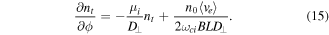
Here simple asymmetric model is 1D in the z direction (see sketch figure 1), the probe is located at zpr. = 0 and the wall at zw. = Lt, the length of the flux tube is then Lt and  . The probe potential is at V, the space potential is ϕt and the wall is grounded. The section of the tube on the wall side is Sw., and the section at the probe is Spr. with Spr. ≤ Sw.. We assume constant density in the tube, nt, and no loss in the perpendicular direction. Thus, the stationary (∂tn = 0) continuity equation writes:

For homogeneous current density across both ends, using Gauss's theorem by integrating equation (1) over the whole flux tube gives:

Ion current density is the Bohm flux,

and for electron it is given the Boltzmann equilibrium with the local potential,
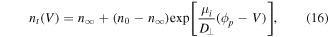
Introducing the electron saturation current as  and the floating potential,
 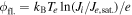 , equation (2) becomes:
where Σ = Sw./Spr.. Finally, the collected current on the probe is

Thus, using equation (3) in (4) one will get:
The asymmetric double probe I(V) characteristics from equation (5) is plotted in figure 2.

Figure 2. Theoretical and normalized asymmetric double probe characteristics for several values of Σ. For  the characteristics are called 'asymmetric', and for
  they are very similar to classical Langmuir characteristics (Sw. is the surface of the whole vessel in that case).
Download figure:
Standard image High-resolution imageIn this paper, we investigate the general behaviour of 'bumped characteristics' with respect to several parameters, such as the amplitude of the magnetic field, the gas pressure or the RF power input. We also propose a new explanation of the bump, with the aim of a better understanding of Langmuir probe measurements in magnetized plasma. In the first part section 2, the experimental set-up and the plasma parameters (mean free paths, Larmor radii, etc.) are detailed. Then the main experimental results are shown in section 3, where the behaviour of the bumps was studied with respect to the amplitude of the magnetic field in section 3.1, the angle ϑ between the probe and  in section 3.2, the RF-power input in section 3.3, the probe position with respect to the RF-antenna in section 3.4 and finally the He pressure in section 3.5. In the following, section 3, a method is proposed to determine the plasma temperature and density with conventional methods (when no magnetic field is present). Finally, the origin of the bump characteristics is explained thanks to a fluid model in the last section.
2. Experimental setup
Experiments were performed in the ALINE [26, 27] (A LINEar plasma device) reactor (see figures 3 and 4). The cylindrical chamber is 1 m long and 30 cm diameter. The typical discharges presented here are generated by a RF-antenna at νRF = 25 MHz (but the amplifier frequency can be tuned from 10 kHz to 250 MHz), and the RF-power is in the range 20–200 W (though 0–600 W is achievable). The amplifier is directly connected to the antenna (direct coupling, so the average potential on the antenna is 0 V). The cathode is at the centre of the vessel has a radius of 4 cm and is 1 cm thick.
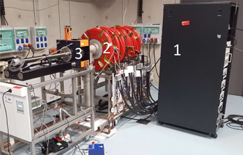
Figure 3. Photograph of the ALINE plasma device. The cylindrical vessel (2) is 1 m long and 30 cm diameter. Six coils (in red) are placed equidistantly along the axis, around the chamber to generate a quasi-homogeneous and uniaxial magnetic field along the axis of the cylinder. The power supplies for the coils and the RF antenna are placed in the rack (1). The antenna is in the middle of the vessel. The arm (3) holding the hidden Langmuir probe along the vessels axis was developed by Cryoscan and is able to perform 3D translations (along the axis, up/down and left/right). Note that the arm is always parallel to the axis of the cylinder.
Download figure:
Standard image High-resolution image
Figure 4. Schematic representation of the plasma device designed by Cryoscan. The gas inlet is on the top-right end of the device (on the opposite of the pump).
Download figure:
Standard image High-resolution imageSix circular coils generate an axial magnetic field from 0 to about 100 mT (the current in the coils is in the range 0–200 A). Helium gas was used for all discharges with a pressure in the range between 1.2 and 40 Pa for this study, which allows the study from collisionless to collisional regimes.
The cylindrical Langmuir probe tungsten tip used in measurements has a length Lp of 1 cm and a radius rp of 75 µm. To enable measurements in a RF plasma, the probe is RF-compensated [7, 28]. For each I(V) characteristics, a voltage ramp from −70 to 70 V is swept 20 times at a frequency of the order of 65 kHz. Hence, the measurement frequency is much slower than RF-oscillations and all plasma frequencies (ωc and ωp), and thus, can be seen as 'stationary' with respect to the plasma dynamics.
The position of the probe tip is given with respect to the middle of the antenna (y = 0 and z = 0). All measurements were performed at z = −60 mm along the axis of the cylindrical chamber and y = 40 mm above the antenna. The arm holding the probe is parallel to the axis of the cylindrical vessel, and only the tip is tilted ϑ with respect to the magnetic field lines (see figure 5). ϑ ∈ [0, 6, 12, 18, 40, 94]° angles were used for the study.

Figure 5. Tilted cylindrical Langmuir probe with an angle ϑ = 12° with respect to  (which is assumed homogeneous and constant in the whole probed volume). The position of the probe is z = 0 and y = 5 mm on this photograph. The value of the angle with respect to the antenna was measured thanks to the open source GeoGebra software.
Download figure:
Standard image High-resolution imageMoreover, the arm (see (3) in figure 3) is able to move the probe tip inside a volume (see the red dashed box in figure 6) to get three-dimensional measurements of plasma parameters. Solving Biot–Savart law in the whole vessel gives the magnetic field topology. Figure 6 shows the result of the computation. Let  be the averaged modulus inside the workable volume: in this paper we assume uniaxial (along z, the axis of the reactor) and constant magnetic field (the deviation from the averaged value being less than 3% in the probed volume). In the following
  , and
, and  .
.

Figure 6. Magnetic topology in the ALINE plasma device. The gray rectangle at the bottom represents the RF electrode (also called RF antenna), the long black rectangle and the narrow line at its end at r = 4 cm represents the probe and its arm at probing position (x, y, z) = (0, 40, −60) mm. The red dashed box delimits the workable volume. White arrows represent the local magnetic field vectors.
Download figure:
Standard image High-resolution imageIn low pressure conditions, p = 1.2 Pa, the plasma can be considered as collisionless. Indeed after the values listed in table 1, electron mean free path is greater than the probe dimensions [6], i.e. λe,mfp ≫ rp and Lp. Ions can be considered as unmagnetized for the probe since  ≫ rp. Note that an electron needs a parallel velocity over Lpωce/2π ≈ 2.8 × 10⁷ m s−1 to overfly the probe without completing a cyclotron period: at this velocity the
  , which means that almost all electrons complete an entire turn over the length of the probe. The electron collection can thus be seen as the intersection of the 'cyclotron disk' (
 ) with the probe for parallel inclination in collisionless regimes.
Table 1.
Plasma parameters for  = 100 mT and p = 1.2 Pa. Note that probe dimensions are rp = 75 μm and Lp = 1 cm, ρc is the Larmor radius, λmfp is the mean-free-path for charged particle/neutral collisions, νc the cyclotron frequency (ωc/2π), νp the plasma frequency and
  the charged particle/neutral collision frequency [29, 30].
| Quantity | Ions He+ | Electrons e− | |
|---|---|---|---|
| T | (eV) | 0.026 | 2–4 |
| n | (m−3) | 5–50 × 1015 | 5–50 × 1015 |
| ρc | (μm) | 400 | 37–83 |
| λmfp | (cm) | 1.50 | 2–4.5 |
| νc | (Hz) | 380 × 103 | 3 × 10⁹ |
| νp | (Hz) | 7–23 × 106 | 635–2000 × 106 |
| νcol.N | (Hz) | 88 × 103 | 38–85 × 106 |
3. Experimental study
Scans over B, ϑ, RF-power, y-position and pressure were performed and main results are presented here. If not specified the probe tip position is set by default at y = 40 mm and z = −60 mm, and the pressure at 1.2 Pa.
3.1. Influence of the magnetic field
I(V) characteristics for all inclinations of the probe tip have been plotted for several values of  and for a 200 W-RF power input in figure 7. Without magnetic field (figure 7(a)), the 'classical' I(V) is recovered, because the plasma is seen as isotropic by the probe. The slight differences between all six curves come from small variations on the plasma conditions, due to the fact that the change of inclination requested to open the chamber between each measurement (uncertainties within 5% due to the gas pressure gauge, thus the RF coupled power which is sensitive to the pressure may not be exactly the same).

Figure 7. Evolution of the I(V) characteristics at 200 W-RF power, at position y = 40/z = −60 mm with increasing  from 0 (a) to 95 mT (d) for all six ϑ inclinations, 1.2 Pa He. Potential range of the measurements were −70 to +70 V, but the purpose of the study is not the ion part so only the range [0, 70] V is displayed here. Note that the current range changes for each graphs.
Download figure:
Standard image High-resolution imageThe shape of the I(V) changes drastically in the presence of a magnetic field as depicted in figures 7(b)–(d). The slope of the exponential part and the electron saturation current one as well as the ratio Ie/Ii are strongly affected by the addition of a magnetic field [11]. Note that the increase of Ie with the magnetic field is due to a better coupling of the RF power and to better confinements. More generally, it can be seen that the overall shape of the characteristics are qualitatively close to the double probe/tanh-shape ones modelled by equation (5). For small angles (ϑ ≤ 12°), the characteristics even display a bump between the exponential and the saturation parts. The bump's overshoot amplitude and the change in the slope between the exponential part and the electron saturation regime is emphasized and steeper with larger  .
.
3.2. Influence of probe inclination
For a probe inclination of 18°, the measured I(V) characteristic looks like the 'tanh-shape' as explained previously. For higher inclination angle, the electron current does not saturate (due to sheath expansion) and for lower inclination angle, there is a bump. The only difference between all these different cases is the width of the flux tube that scales as  . The probe area facing magnetic field lines (see figure 5) is written as follows:

which can be scaled as  because Lp ≫ rp.
For ϑ = 0° at 100 mT, rp ≈  , therefore, the probe surface facing the magnetic flux tube is comparable to the 'cyclotron area' (
 ): in this case of grazing incidence, a bump arises on the measured characteristics. By increasing the angle, the facing surface increases (whereas the cyclotron area remains constant) and the amplitude of the bump decreases, and even disappears for larger angles. One can suggests that the flux tube narrowness comparable to the cyclotron area could explain the bump. However, it remains even if Sface ≫ Sce (when ϑ > 5°), therefore another mechanism should be invoked in order to explain the presence of the bump.
We performed a series of experiments with a power input in the range 20–200 W in order to quantify the evolution of the characteristics with respect to ϑ. Figure 8 shows the evolution of the current at 70 V, I(V = Vmax = 70 V) or the 'end-current', against  . This end value is used, because the plasma potential is actually unknown, so the comparison of the current at plasma potential is not possible for now.
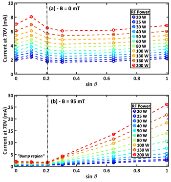
Figure 8. Evolution of the collected current at 70 V with the sine of the inclination angle ϑ without magnetic field (a), and with magnetic field (b) of amplitude 95 mT, 1.2 Pa He. The left region is the 'bump region', where a bump is measured ( ). The line is a guide for the eye.
Download figure:
Standard image High-resolution imageWithout magnetic field (figure 8(a)), the end-current is constant for any inclination as explained previously. Moreover by increasing the RF-power, the overall collected end-current also increases, because the power also increases the plasma density (I ∝ ne) as expected.
In the presence of a magnetic field of 95 mT (figure 8(b)) two regimes are evidenced: the region where there is a bump ( ) and the region with an asymmetric double probe behaviour (above 12°). In the former region, the end current is proportional to
  , as the width of the magnetic flux tube: the sine dependence of the current collection is verified. But in the 'bump region', the collected end-current remains approximately constant with ϑ for any RF-power. Since the collected current is proportional to the product of the density with the collecting surface, neScoll. (assuming
 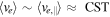 ), the increase of the angle also increases Scoll., so to keep constant collected current, the electron density in the flux tube should decrease. This is in a good agreement with figure 9(b): in the presence of a magnetic field, and if there is a bump on the characteristic, the density is lower than in the absence of a bump (going from ne ≈ 5 × 10¹⁵ m−3 with a bump to ne ≈ 15 × 1015 m−3 without a bump at 200 W RF power). This density difference is enhanced for higher power. However, for lower power the density remains approximately constant at all inclinations.

Figure 9. Evolution of the density measured with the method described in the next section, in same conditions as in figure 8 with magnetic field (a) and without magnetic field (b) of 95 mT. As expected, the density is kept approximately constant in the absence of magnetic field, but we notice a sharp change in the density between the 'bump-' and the 'no-bump-region' in the presence of magnetic field at higher power. The line is a guide for the eye.
Download figure:
Standard image High-resolution imageHowever, the evolution of the electron temperature with respect to the inclination angle (figure 10) is impossible to explain straightforwardly. Indeed the electron flow collected by the probe is the combination of two populations: the parallel and the perpendicular to B flow, having each its own temperature (i.e. Te∥ and Te⊥ resp.). Our method gives a kind of average of both. Unfortunately, the electron energy distribution function, which could help us to understand the plot, is too noisy to be exploited (even after some filtering such as Stavitzky Golay, or Fourier analysis). The explanation of this plot is still an opened question for further studies.
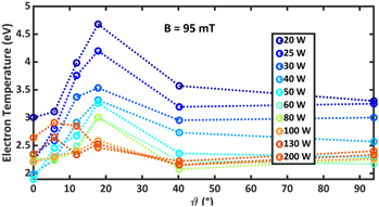
Figure 10. Evolution of the computed electron temperature (see next section for the used algorithm) with respect to the inclination of the probe at 95 mT magnetic field amplitude. The line is a guide for the eye.
Download figure:
Standard image High-resolution image3.3. Influence of the RF-power
As shown in the last subsection, increasing RF-power also increases the overall density. To track the bump evolution with RF-power regardless to the density change, it is convenient to normalize the I(V) to the end-current value I(V)/I(70 V). In figure 11 are depicted the normalized probe characteristics at  = 95 mT for all inclinations and for several input RF-power, figures 11(a)–(c).
Figure 11. Normalized I(V)/I(Vmax) characteristics at 95 mT, for every inclination angles, 1.2 Pa He. RF-power is fixed at (a) 20 W, (b) 80 W and (c) 200 W. On each graph is also plotted (on dashed lines) the mean saturation linear curve with its slope.
Download figure:
Standard image High-resolution imageAlthough the end current is proportional to the collecting surface (which is  ), the normalization removes this dependence and all angles can be compared. The electron saturation part, directly connected to the sheath extension, is then the same for every angles, as shown in figure 11. In figure 11(a), for 20 W there is no bump at 12°, contrary to figure 11(b) for 80 W. The current at the bump position is also larger than the end-current in figure 11(c). Moreover, the increase of the power increases the amplitude of the bump and its width.
One can suppose the existence of perpendicular (to  ) RF currents, pumping the flux tube connected to the probe: this idea is used to derive a fluid model in section 4 to recover the bump analytically. In addition, as depicted in figure 8(b), increasing the power does not increase the end-current in the 'bump region', corroborating the former assumption. These RF currents, when averaged over one RF period, exhibit a net DC perpendicular contribution [31], acting as perpendicular DC currents, which have already been investigated in previous models [22, 23] to explain the depletion and saturation currents of biased flux tubes.
3.4. Influence of the probe position
The position of the probe is also an important parameter. It is initially placed relatively far from the antenna to have a homogeneous plasma around the probe. Indeed, near the antenna, the  effect is larger and the plasma denser. That is why, there is a thin plasma layer above, and below the antenna (see photograph in figure 12). Moreover, at this RF-pulsation ions do not react to the quick potential change near the antenna, whereas electrons do [32] (ωpe > ωRF > ωpi).
Figure 12. Photograph from 1.2 Pa He pressure plasma around the RF antenna operating at 100 W with  = 80 mT magnetic field. The magnetic confinement generates this double player plasma aspect around the probe. Far enough from the antenna the density is homogeneous.
Download figure:
Standard image High-resolution imageTo make sure that the inclination of the probe scan a homogeneous plasma in a range of  around the probing position in the y direction, measurements along the y axis were performed at fixed z = −60 mm position and for ϑ = 0°. Power was fixed at 100 W-RF,
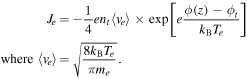
  = 80 mT in 1.2 Pa He plasma. All characteristics in figure 13 depicted a bump, where the plotted parameters are the floating potential ϕfl., the bump potential Vbump and the bump current Ibump. Dote suggested the bump potential to be near the plasma one [15, 19, 20]. According to Dote's assumption and using the combined potential drops in the sheath and the collisionless pre-sheath [1], one can write the potential drop between the plasma and the floating probe potential for cold ions (Ti/Te → 0) as:
with Te in eV. For all previous measurements at (z = −60 mm, y = 40 mm), using the approximation ϕp ≈ Vbump gives Te ≈ 1.30 eV (which is a typical value in ALINE magnetized, plasma [26, 27]).
Figure 13. Evolution of measured parameters (floatting potential ϕfl., bump potential Vbump and bump current Ibump) along the y axis at z = −60 mm, 100 W-RF, 80 mT and 1.2 Pa (see double arrow  in figure 12). The gray region represents the region where the probe faces the antenna (antenna extension is z ∈ [−40, 40] mm and y ∈ [−10, 0] mm), the purple regions represent the denser plasma region (see photograph in figure 12). For comparison Te ∝ Vbump − ϕfl. is also plotted.
Download figure:
Standard image High-resolution imageAs seen in figure 13, 1 cm around the y = 40 mm position, the homogeneity hypothesis (almost constant Te and ne in the probing area) can be applied in the experimental conditions and the probe inclination scans the same plasma parameters at all angles. Finally, this last figure also highlights the fact that current and temperature (as defined in equation (7)) increases by a factor of ∼7 in the bright regions (see photograph depicted in figure 12), near the antenna.
3.5. Influence of the pressure
For a magnetic field of 80 mT, and an input power of 80 W-RF, measurements were performed with a probe parallel to the field line (ϑ = 0°) in a He pressure range from 1.2 to 40 Pa. All characteristics are plotted figure 14.
Figure 14. Tridimensionnal representation of the I(V) characteristics in all considered He pressures from 1.2 to 40 Pa for 80 W-RF power and  = 80 mT. In the V = 80 V plane are plotted the end currents at ±70 V and the bump current. In the I = −3 mA plane are plotted the floating and the bump potentials. Last bump is measured at 9.32 Pa. If no bump is measured, Ibump corresponds to the point where
 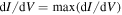 , i.e. the current at 'classical' plasma potential.
Download figure:
Standard image High-resolution imageWhen pressure increases, the bump gets narrower and its amplitude diminishes. Above 9.32 Pa, the bumps disappear and the I(V) characteristic turns into an asymmetric double probe one.
That's why one can separate the pressure range in 2 regimes:
The low collisional regime from 1 to 10 Pa. At these pressures the electron–neutral collision frequency  is lower than the electron plasma frequency νpe, and lower than the electron cyclotron frequency νce (see table 1) and of the same order than the RF frequency. For example at 1 Pa
  MHz [29]. In the same way the ion-neutral collision frequency
  is much lower than the ion plasma frequency νpi, and lower than the ion cyclotron frequency νci up to 4 Pa so that ions are considered as magnetized in the first half of the low collisional pressure range. In this range the classical perpendicular diffusion falls down and perpendicular currents are able to deplete strongly the flux tube while the typical scale length of these current is higher than the radius of the probe, which is the case here because ρci ≫ rp. In a quiet plasma, as we have in ALINE, such a behaviour can be seen, while in Tokamak edge plasma anomalous transport can still prevent the biased flux tubes to deplete.
In the collisional regime (P > 10 Pa),  remains lower than νce and νpe, but much higher than the RF frequency. RF electron current are then lowered by collisions. And ions are no more magnetized because
  , which favours their perpendicular diffusion while ion perpendicular current are lowered in the same time, filling the lack of density caused by the probe collection and cancelling the bump on the characteristics. For the highest pressures, the flux tube for ions disappears and the I(V) looks like an unmagnetized one [14].
In the intermediate case of partially magnetized ions, the I(V) looks like a double symmetric probe characteristics. The electron saturation current collected by the probe depends also on the competition between perpendicular DC and RF currents and the cross diffusion of ions due to collisions.
4. Theoretical approaches
In the first part of this section, we provide a quantitative comparison of three different methods used to extract both ne and Te from bumped characteristics. In a second part, we show by using a fluid model that, the bump in the I(V) curves in a presence of a magnetic field, can be explained by mean of density depletion within the tube flux connected to the probe and to the opposite wall of the reactor.
4.1. Density and temperature data processing
Extracting electron density and temperature from I(V) characteristics is far from simple. But if the measurements are done in the presence of a magnetic field, the exploitation are even more difficult. The challenge lies on the presence of the bump, whose existence, shape, location and amplitude depend on several plasma parameters 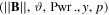 (see sections 3.1–3.5).
The first problem with bumped characteristics is the uncertainty on the position of the plasma potential. Indeed, the plasma potential is actually the local plasma potential with respect to the perpendicular direction to the magnetic field. It is usually found by assuming that, at the plasma potential V = ϕp,  , which is equivalent to
  [2, 3] (this is called the 'classical method' in the following). Another method based on the intersection of the linear fits of the exponential part and the electron saturation one has also been suggested and used in a previous study [17]. It was finally suggested that, in the context of bumped characteristics, the bump potential is at the plasma potential [15, 19]. Thus, three methods are available, in order to determine the plasma potential and we propose to compare them, for different inclinations, in a single 100 W-RF plasma, with
  = 80 mT and p = 1.2 Pa, whose characteristics are depicted in figure 15(a).

Figure 15. Results of the electron temperature and density calculation on bumped characteristics with the described iterative model: (a) I(V) of plasma at 100 W-RF, 80 mT and 1.2 Pa for different probe inclinations and all methods are represented for the position of ϕp ( classical,
  intersection,
  bump). The dashed line is the fit of the electron saturation current with respect to equation (8)—(b) and (c) Te and ne against inclination angle with collecting surface correction—(d) and (e) Te and ne against inclination angle without collecting surface correction, Scoll. = Sprobe (Te remains the same though).
Download figure:
Standard image High-resolution imageIn the context of the 'intersection method' we linearised the exponential growth as 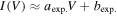 , and fitted the electron saturation current with the formula:

with the  term similar to one of the OML approach, which gives a relatively good fit with experimental curves. This equation is only able to fit the saturation part, i.e. the end of the I(V)—far from the bump potential range. Only the last 20 volts of each I(V) were used for the fitting, see figure 15(a).
We used an iterative method, in order to determine both ne and Te with the plasma potential ϕp, the current at plasma potential Ip, floating potential ϕfl., magnetic field and probe inclination as input parameters. First, a raw approximation of electron temperature is done, supposing 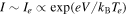 for V ≤ ϕp in the exponential part. Applying a linear fit on ln I(V) one will find a first value of Te. From now one starts the iterative loops: this electron temperature value allows a computation of a gross value of ne since, at plasma potential,
  . The value of Se is not the probe surface, even at plasma potential (where there is no sheath), because of the cyclotron motion. That is why it is assumed that the collecting surface is the probe surface facing
  plus a layer thick of Nelr.
 (i.e. some Larmor radii—Nelr. being the number of electron Larmor radii connected to the probe):
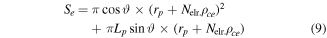
by replacing  in equation (6). It is assumed that this equation takes into account the perpendicular motion of electrons along the magnetic field lines connected to the probe.
With Te and ne, it is possible to compute the electron Debye length λDe and the ion sheath thickness using the Child–Langmuir law (since  and that Zhu's corrections [33] for cylindrical geometry only bring minor changes in opposition to its complexity), knowing,
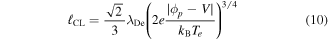
for V ≤ ϕp. Since ions are supposed unmagnetized, the collecting area for ions is

It is then possible to compute the ion current for V ≤ ϕp, using the Bohm flux formula, Ii = 0.61 × enecsSi. So, the updated electron current Ie = I(V) − Ii can be calculated. Taking again the log-scale of this new electron current gives a new more accurate value of Te. The loop starts over again, and ends if temperature values converge (i.e.  , ε being given by the user).
Equations giving Se and Si (equations (9) and (11) resp.) take into account the sheath extension for magnetized electrons and unmagnetized ions. To take into account the inclination of the probe, and find reliable plasma parameters, one should also multiply the total current by a geometric factor of  from equation (6) giving a dimensionless factor of
 ![$1/(\cos \vartheta +[{L}_{p}/{r}_{p}]\times \sin \vartheta )$](https://content.cld.iop.org/journals/0963-0252/29/3/035007/revision2/psstab56d2ieqn69.gif) . This allows the recovering of the same amplitude for all bumped I(V). The extracted values of ne and Te are plotted in figures 15(b) and (c) using this correction, and plotted in figures 15(d) and (e) without the correction (ne strongly decreases with the angle). From figures 15(b) and (c) it is clear that the classical ϕp-determination method gives the more reliable values of temperature and density (the deviation of Te values between each inclination is negligible compared to other methods). We have then Te ≈ 1.2 eV and ne ≈ 1.3 × 10¹⁶ m−3. Since the OML model remains valid in RF-plasmas [34], and that ions are unmagnetized, we extracted
. This allows the recovering of the same amplitude for all bumped I(V). The extracted values of ne and Te are plotted in figures 15(b) and (c) using this correction, and plotted in figures 15(d) and (e) without the correction (ne strongly decreases with the angle). From figures 15(b) and (c) it is clear that the classical ϕp-determination method gives the more reliable values of temperature and density (the deviation of Te values between each inclination is negligible compared to other methods). We have then Te ≈ 1.2 eV and ne ≈ 1.3 × 10¹⁶ m−3. Since the OML model remains valid in RF-plasmas [34], and that ions are unmagnetized, we extracted  m−3 (which is within the typical errorbar for OML model) and
  , which are overestimated compared to the previous method.
By comparison, in the absence of magnetic field, the bump method to find the plasma potential makes no sense (since there is no bump) and both classical and intersection methods are alike and give the same value of the plasma potential. Therefore the self-consistent algorithm gives an electron density of the order of 5.32 × 10¹⁵ m−3 and an electron temperature of 3.47 eV (for the same discharge parameters as with  ).
).
4.2. Fluid model approach
As suggested by Mihaila and Rozhansky [16, 23], the bump on I(V) characteristics could be induced by density depletion within the flux tube.
The cylindrical flux tube connected from the probe to the reactor's wall is filled by electrons using a single channel, which is the lateral area of the cylinder. Due to magnetic confinement and for grazing incidences, the perpendicular current arises thanks to collisions with neutrals. During a I(V) measurement for V > ϕp, one pumps the electrons inside the flux tube, which makes the local electron density decreases. If the pumped electron current is larger than the refill perpendicular one, then the collected current at the probe decreases with phi (the bump origin). But when the probe potential is increased further, the sheath extent around it also increases, which artificially makes the cylindrical flux tube diameter wider. Consequently, when V ≫ ϕp, the electron perpendicular current compensate the pumped one and the collected current increases again. Now for larger incidences, the perpendicular current always overcomes the pumped one, which explains the experimentally observed disappearance of the bump for ϑ > 12°.
In the meantime, there is another mechanism involving mainly ions: it is the plasma pumping via perpendicular ion current due to the positive biasing of the flux tube with respect to the surrounding plasma potential. This mechanism has already been invoked to explain the early electron saturation of the I(V) characteristics in the case of planar probe [23] in magnetized plasmas. The typical scale length of these perpendicular ion currents is the ion gyroradius. To explain the bump, this mechanism can be divided in three regimes occurring when the probe potential overcomes the plasma potential:
- 1.When the transverse (perpendicular to
 ) ion current is lower than the electron saturation current collected by the probe, the space charge of the sheath is electropositive and consequently the flux tube potential 'follows' the probe potential. The density depletion can first appear in that regime.
 - 2.When the transverse ion current is exactly equal to the electron saturation current collected by the probe, the sheath between the probe and the flux tube disappears and the collected current can decrease because the flux tube density decreases with the probe potential.
- 3.Finally when the transverse ion current is higher than the electron saturation current collected by the probe, electrons must be accelerated in the sheath to balance the ion current and thus the sheath drop is reversed. The sheath space charge becomes electronegative and the flux tube potential tends to saturate compared to the probe potential. This regime accounts for long and thin flux tube.

Nevertheless, plasma diffusion is more and more efficient as the flux tube is widening. So in the third regime, with the saturation of the flux tube potential, the pumping also saturates and the density depletion can be cancelled resulting in a classical increase of the current in the last part of the I(V) characteristics (beyond the bump).
Finally there is an optimum point for which the pumping is maximum compared to cross diffusion, and this is at this working point the bump appears to be the higher because of the strong negative slope just following the maximum of the bump. Actually, the bump does not mean there is an increase of current compared to an I(V) characteristics with no bump, on the contrary it means a decrease of current.
The complexity of the phenomenon can only be explained by a mass and current conservation taking into account the growing of the flux tube radius with the potential.
The model
The establishment of the potential and density structures in a magnetized plasma is far from simple and out of the scope of this article. To understand the behaviour of a magnetized plasma during a Langmuir probe measurement, we assume a perfectly magnetized plasma for electrons (they do only move along field lines whereas ions can leave the flux tube though transverse conductivity and can join it thanks to transverse diffusion, see figure 16). The flux tube is assumed homogeneous in the magnetic field direction (z-direction) and well delimited in the radial direction from the bulk plasma. Its length is L and delimited by the probe on the one side, and the vessel wall on the other side.

Figure 16. Sketch of the fluid model. The flux tube is delimited by the dashed line. The inclination ϑ is 0°.
Download figure:
Standard image High-resolution imageRozhansky et al [23] showed that the ion flux tube has a characteristic radius of  , and a length L (this ion flux tube connected to the probe also contains the electron flux tube of radius
  ). To provide an analytical and comprehensible solution, the case ϑ = 0° is considered, that is, the facing surface of the probe,
  is negligible compared to the ion flux tube section
  . For greater inclination angles, the probe radius must be taken into account, making it impossible to provide an analytical resolution.
Due to their cyclotron motion, electrons are trapped in both ion and electron tubes and can only leave them through the ends, producing a parallel net current of  . To ensure current and quasi-neutrality conservation in the ion tube, there must be a perpendicular ion flux through the cylindrical surface so that,
  (corresponding to Γ∥e in figure 16). In this regime, where the perpendicular current can be higher than the electron saturation current on the probe, the potential gap can reverse in front of the probe (electronegative sheath) accelerating electrons and repelling ions. Thus, one can neglect the parallel ion flux on the probe side (in the case of an electropositive sheath, the ion current on the probe surface can also be neglected compared to electron current, still assuming that the electron current is close to its saturation value).
In the following we use current continuity for ions in order to obtain a first order ODE that gives the density of the flux tube with respect to the probe potential. Using Laframboise's theory, this tube density (or 'local plasma density') gives the electron fraction that will be collected by the probe regarding its potential V. An analytic expression of the collected current can be then provided.
As shown in the last sections, the pumping is enhanced by perpendicular (to  ) RF and DC currents [21, 22]. But periodic RF current can be reduced to an averaged DC over one a period. That is why the model is steady state, and only DC quantities are considered. Finally, to prevent the tube density to drop to zero, we assume the presence of a source term S0, so that,

where n0 is the bulk plasma density (outside the ion flux tube region) and nt, the ion flux tube density (n0 ≥ nt). This term fills the tube at the same rate electrons leave it from both ends (which is an overestimation of the 'real' S0 source term).
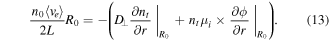
From the stationary ion continuity equation, we have 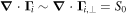 . Perpendicular ion flux is separated in two parts (see figure 16): lateral mobility
  and the diffusion flux
  . Integration of all ion fluxes through the whole tube using Gauss's law gives:
In the presence of a strong radial electric field (and especially in a cold plasma), the ion drift velocity is larger than the thermal velocity, thus  =
= 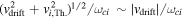 =
=  (all at R0). Recalling that
  , equation (13) rewrites as,
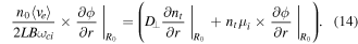
Now using the chain rule,  , one will get the following first order ODE at the radius r = R0:
The perpendicular mobility can also be written as a conductivity depending on the current nature (collision, inertial, viscosity, anomalous, ...). With the initial condition of nt(ϕ = ϕp) = ne since there is no sheath nor spatial potential variation at plasma potential, one will get:
where V is the probe potential and  . Here we assumed that the flux tube potential equals the probe one. Although generally, ϕt = f(V) ≥ V > ϕp, with f a cumbersome function [21].
Equation (16) exhibits an exponential decay of the density with V. This strong depletion of the flux tube as soon as the biased potential of the tube is higher than the surrounding plasma potential is needed to see the bump rising. For lower decay (for ex. ∼1/(V − ϕp) or  ) the bump does not appear because of the expansion of the sheath which increases the lateral surface of the flux tube and hence the total perpendicular current more rapidly that the density is depleted. This also explains why at higher probe potential value, when the exponential decay saturates, the current rises up again due to sheath expansion. Actually there is a competition between the diffusion D⊥ across the lateral surface of the tube versus the perpendicular current due to ion mobility μi as it can be seen in equation (16).
After that, to fit the sheath expansion above Vp in a magnetic field parallel to the probe, one uses the Laframboise [9] model which showed that the portion of plasma density actually touching a probe and thus collected, neff., is given by the relation,
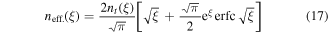
for ξ = e(V − ϕp)/kBTe. Finally, the collected current on the probe is simply given by

where Se is given by equation (9), and the number of electron Larmor radii (Nelr.) is given as fitting parameter.
This model is compared with the experimental data in figure 17 for a magnetic field of 57, 70 and 100 mT in a 200 W-RF and 1.2 Pa helium plasma (the probe was parallel to  ). For V < ϕp the exponential
  part of the electronic current is considered.

Figure 17. Comparison of the 1D fluid model with the experiment. Probe had ϑ = 0° inclination angle in 200 W-RF plasma at 1.2 Pa for several  . The ion part is fitted using OML theory (i.e. Ii2 is a linear function).
Download figure:
Standard image High-resolution image
The fitting of bumped characteristics leads to anomalous transport coefficients [2] (see table 2). Indeed, μi ≈ 20 m2 V−1 s−1 and D⊥ ≈ 40 m2 s−1 are the outputs for the three depicted curves. This highlights the fact that the flux tube evolves in a forced regime: because the parallel current saturates at the electron saturation current, this regime involves anomalous transverse transport coefficients in order to satisfy current conservation in the flux tube.
Table 2. Outputs values for temperature, density, mobility and diffusion obtained from the fitting of a bumped I(V) (see figure 17), measured with a probe align with magnetic field lines (i.e. ϑ = 0°).
| B (mT) | 80 | 70 | 57 |
| μi (m2 V−1 s−1) | 19.5 | 26 | 20 |
| D⊥(m2 s−1) | 39 | 52 | 50 |
| n0 (1015 m−3) | 8.0 | 6.0 | 3.1 |
| Te (eV) | 2.7 | 2.5 | 3.5 |
The number of Larmor radii, Nelr. goes from 0.1 to 5 with increasing  in equation (9). The limit density in the flux tube,
  is close to n0/10: that means that the measurement heavily depletes the magnetic flux tube. Moreover, the model suggests that the plasma potential is on the top of the bump as proposed by Dote and Mihaila: the pumping mechanism starts when V > ϕp according to the theory. Since electrons are way much mobile than ions along B, as soon as the probe potential is above the plasma potential, electrons of the flux tube are flushed towards the probe. Moreover, as pointed out by equation (3), the flux tube itself has its own potential (slightly above the bulk plasma potential) since it is connected to the probe and thus somehow biased.
Finally, according to this theory, the prior parameter is actually the probe surface facing the magnetic field lines (i.e. the width of the magnetic flux tube). Therefore, a bump could appear on a plane probe characteristics or a spherical probe characteristics as well, if the facing surface is small enough corresponding more or less to a disk surface having a radius of the order of  .
.
5. Conclusion
Langmuir probe measurements in the presence of a magnetic field are of a paramount importance in plasma physics. Understanding and exploiting I(V) characteristics from a cylindrical Langmuir probe in such conditions is difficult, especially due to the presence of a bump in the curves for grazing incidences of the cylindrical probe with respect to the magnetic field lines. In this paper, the evolution of the I(V) characteristics with respect to several discharge parameters (magnetic field amplitude, probe inclination, and pressure) was studied, in order to provide a better understanding of cylindrical Langmuir probe measurements in magnetized plasmas.
We showed that the presence of the magnetic field changes the general shape of the I(V) curves, because of the breaking-up of the plasma isotropy: the particles are not collected by the probe from all possible directions anymore but from a flux tube, connected to it from one end, and to the reactor's wall to the other. That is why the general shape of the characteristics tends to an asymmetric double probe (or tanh-shaped) one. We also showed that for grazing incidences of the probe with respect to B, a bump arises between the exponential part and the electron saturation current one. The bump vanishes as the probe inclination is increased, or if the magnetic field amplitude is reduced. It is also dependent on collisional processes, because its amplitude decreases, when the gas pressure increases. Finally, increasing the RF-power at the antenna heightens the bump amplitude, and can even make one appearing on the characteristics.
We argued that a probe measurement pumps electrons from their flux tube while ions are expelled in the perpendicular direction (the electron current is mainly parallel to magnetic field lines). This density depletion as soon as probe potential V overcomes the plasma one ϕp (i.e. as the probe starts to attract electrons) can explain the presence of the bump. This hypothesis is strengthened by the pressure effects on the probe measurements: increasing the gas pressure (thus increasing collisions and therefore, perpendicular diffusion fluxes), makes the bump vanish. By using a fluid model, we corroborated the pumping mechanism of density (due to a competition between mobility and diffusion) and validated the assumption of density depletion in the flux tube connected to the probe. Nevertheless this assumption is not enough to make appear the bump, the density decay in the flux tube must be stronger than the perpendicular expansion of the flux tube with V, that is why the exponential decay from our model is needed.
We have finally compared different methods for extracting both ne and Te from bumped characteristics, which are not very usual in the context of probe measurements. We showed that the classical method of plasma potential determination (where dI/dV is maximum) stays the most reproducible method to access this important parameter, although previous studies argued that the plasma potential coincides with the bump one. A lot of work is still needed to provide a complete theory that exploits bumped characteristics, especially to know the good collecting surfaces of the probe, and the good mobility and diffusion parameters to put in the model.
Acknowledgments
This work has been carried out within the framework of the French Federation for Magnetic Fusion Studies (FR-FCM) and of the Eurofusion consortium, and has received funding from the Euratom research and training programme 2014–2018 and 2019–2020 under grant agreement No 633053. The views and opinions expressed herein do not necessarily reflect those of the European Commission.