
Abstract
Image fusion technology combines information from different source images of the same target and performs extremely effective information complementation, which is widely used for the transportation field, medicine field, and surveillance field. Specifically, due to the limitation of depth of field in imaging device, images cannot focus on all objects and miss partial details. To deal with this problem, an effective multi-focus image fusion method is proposed in this paper. We interpret the production of the focus map as a two-class classification task and solve this problem by using a method based on the cascade-forest model. Firstly, we extract the specific features from overlapping patches to represent the clarity level of source images. To obtain the focus map, feature vectors are fed into the pre-trained cascade-forest model. Then, we utilize consistency check to acquire the initial decision map. Afterward, guided image filtering is used for edge-reservation to refine the decision map. Finally, the result is obtained through pixel-wise weighted average strategy. Extensive experiments demonstrate that the proposed method achieves outstanding visual performance and excellent objective indicators.
1 Introduction
Image fusion technology combines information from different source images of the same target, which is more conducive to comprehensive access to the target and the scene information. It can significantly improve the deficiencies of a single sensor and improve the clarity of the resulting image. As shown in Fig. 1, image fusion is widely employed in different imaging systems, including multi-focus medical image fusion [1, 2]. Due to the limitation of depth-of-field (DOF) of optical lenses in imaging devices [3, 4], it is difficult to obtain images directly in which all targets are accurately focused. However, lacking image information may seriously affect the understanding of image details. Numerous multi-focus image fusion methods were proposed during the past few decades, which can be roughly divided into transform domain-based methods and spatial domain-based methods [5].

Image fusion in imaging systems. Image fusion technology is widely used in transportation, medicine, and surveillance
For the transform domain-based methods, the multi-scale transform (MST) methods [6] are continuously classic. Early typical the MST-based method is the Laplacian pyramid (LP) transform [7, 8]. Afterward, some representative methods contain the gradient pyramid (GP)-based methods [9] and the morphological pyramid (MP)-based methods [10]. The wavelet transform (WT)-based methods [11] can counteract the defect of LP-based methods. Moreover, the typical MST-based methods were proposed, such as the discrete wavelet transform (DWT) [12, 13], the dual-tree complex wavelet transform (DTCWT) [14], and the non-subsampled contourlet transform (NSCT) [15]. To achieve the better fusion results, sparse representation (SR) was employed in [16, 17], which achieved quite attractive performance.
For the spatial domain-based methods, the weighted average (WA)-based [18] was the most uncomplicated method and utilized directly weighted average of the gray value of pixels about source images. Hereafter, the guided filter (GF)-based methods [19] and the rolling guidance filter (RGF)-based methods [20] were proposed. Since spatial domain-based methods mainly adopt patches as the fuse target [21], patches with different sizes will get different results. Therefore, [22, 23] adaptively selected the size of patches according to the image property. Recently, machine learning (ML) was introduced for image fusion technology, especially the artificial neural network (ANN) which significantly improved the fusion effect as in [24]. Hereafter, [25] pioneered the convolution neural network (CNN) for multi-focus image fusion, it fed two complete source images instead of image patches into the model. CNN’s inherent feature learning characteristics were exploited for feature extraction and classification.
However, the transform domain-based methods often introduce redundant information. To contrast, the MST-based methods are overly susceptible to mis-registration [26]. Furthermore, the loss of source images’ detail is an inevitable problem. For the spatial domain-based methods, although they can achieve an outstanding performance, there are still shortcoming. Owing to the limitation of fusion rule, it is impossible to obtain an excellent classification result [25]. Meanwhile, block artifacts and contrast reduction are long-standing problems for most of the spatial domain methods.
Taking the aforementioned drawbacks into account, we present a novel cascade-forest-based fusion method. The Cascade-forest as a decision tree ensemble method is a part of deep-forest [27], which was proposed by [27] as a classification model. The main innovation of this paper is an efficient improvement of the cascade-forest-based ensemble method for multi-focus image fusion. Our paper mainly affords three contributions, which can be outlined as follows:
This paper proposes a novel multi-focus image fusion method based on the cascade-forest model. Experiments show that our method achieves excellent performance.
Spatial domain-based methods often suffer from the limitation of fusion rule. To address this problem, we interpret the production of the focus map as a two-class classification task and utilize the cascaded-forest model as an effective fusion rule.
For most spatial domain-based methods, they often produce undesirable artifacts around the boundaries between the focused and non-focused regions. To address this problem, we employ the guided image filter to refine the initial decision map for better edge-reservation. In this way, the boundary of fused images achieves a smooth edge transition and fewer artifacts.
The remainder of the paper is organized in the following manner. Related work is discussed in Section 2. We elaborate the proposed method in Section 3. The comparison results are discussed in Section 4. At last, some conclusions are drawn in Section 5.
2 Related work
2.1 The cascade-forest model
The cascade-forest as ensemble learning approach consists of basic learners. To obtain an ensemble model with excellent performance, an individual learner (also called a basic learner) should be “good and different.” According to error-ambiguity decomposition:
where Err denotes the ensemble error, \(\overline {\text {Err}}\) denotes the mean error of individuals, and I denotes mean diversity of individuals. Zhou and Feng [27] open a door towards an alternative to deep neural networks (DNN). The cascade-forest is one of the major parts of [27], which gives a powerful ability that can be comparable to DNN. Layer-by-layer processing, feature transformation and sufficient model complexity are the most critical three ideas for the cascade-forest model, as shown in Fig. 2. Suppose we have two classes that need to be predicted. Consider there are four different ensemble algorithms. Black and blue are random forest and completely random forest, respectively. Let \(F_{IN}\epsilon \mathbb {R}^{m\times 1}\) as the input feature vector and m represent the dimensions of the input features. Features after the first cascade layer concatenates with FIN as features \(F_{1}\in \mathbb {R}^{(d+m)\times 1}\).

The cascade-forest structure. Suppose we have two classes that need to be predicted. Consider there are four different ensemble algorithms. Black and blue are random forest and completely random forest, respectively. Each level of the cascade forest is an ensemble of distinctive classification algorithms. Each algorithm will generate a prediction of the distribution of classes. The final prediction is obtained by layer-by-layer processing
where \(\phantom {\dot {i}\!}H_{\text {CASF}_{1}}(\cdot)\) denotes the first cascade operation, and ⊕ means concatenation operation. \(F_{1}\in \mathbb {R}^{(d+m)\times 1}\) is used as the input features to the second cascade layer, where d represents the dimension of the output features. Then, we can obtain the following operation:
where \(\phantom {\dot {i}\!}H_{\text {CASF}_{2}}(\cdot)\) denotes the second cascade operation. Supposing we have N layers, the output features FN can be acquired by:
where \(\phantom {\dot {i}\!}H_{\text {CASF}_{N}}(\cdot)\) denotes the N cascade operation. At last, the prediction value can be obtained by
where Ave(·) indicates the average operation and Max(·) denotes the maximum operation. The last prediction will be one or zero.
With a cascade structure, the cascade-forest can process data layer-by-layer. Therefore, it allows the cascade-forest to perform the representation learning. Secondly, the cascade-forest can autonomously control the number of cascade layers so that the model can adjust complexities based on the amount of data. Even with small data, the cascade-forest model performs well. More importantly, by concatenating features, the cascade-forest model makes a feature transformation and retains the original features to continue processing. In a nutshell, the model can be concerned as “ensemble of ensembles.”
The model, presented in Fig. 2, is noticed in detail that each level is an ensemble of distinctive classification algorithms. In this paper, we apply four different classification algorithms. Each algorithm will generate a prediction of the distribution of classes. For instance, by calculating the proportion of different classes of training samples that was predicted by each base classifier, then the class vector is obtained through averaging all base classifiers in the same classification algorithm. Extreme gradient boosting (XGBoost) [28] is integrated by classification and regression trees(CART), which is based on boosting ensemble learning and joint decision-making by multiple associated decision trees. Boosting training of the base learner adopting re-weighting and re-sampling. The goal of XGBoost does not directly optimize the entire model. It optimizes the model in steps. The first tree is optimized, and then the second tree is optimized until the last tree is optimized.
Besides, we utilize a completely random forest and a random forest [27]. As we all know, random forest randomly selects n numbers of features from input features as a candidate and then selects the best one through calculating GINI value for splitting. Instead, completely random forest only randomly selects one feature for spite from input features.
Furthermore, in the classification task, there are negative class (zero) and positive class (one). Logistic regression is a typical two-class classification model. We employ logistic regression to increase the diversity of ensemble learning. The objective function of logistic regression is described as:
Among Eq. (6)
where k indicates the number of input samples, q(i)ε(0,1) denotes the label of samples, m represents the dimension of input feature, hΘ(x(i)) is called sigmoid function, \(\frac {\lambda }{2k}\sum _{j=1}^{m}\Theta _{j}^{2}\) is the regularization of loss function, λ is hyper-parameter, x is the input feature vector, and \(\Theta \in \mathbb {R}^{m\times 1}\) as a vector represents the optimization parameters of the model.
In summary, the cascade-forest includes four different types of algorithms to enhance the diversity discussed before. Combining four distinctive algorithms achieves excellent performance. The outstanding classification effect of the cascade-forest has been confirmed in [27].
2.2 Guided filter
Due to the neighborhood processing in spatial focusing measurements, the boundaries between the focused and non-focused regions are usually inaccurate. Especially in the spatial domain, this problem will result in undesirable artifacts around the transition boundary. Similar to [25] and [17], we make use of the GF [29, 30] to refine the initial decision map. The GF has excellent characteristics of edge-reservation, which can be expressed as follows:
where Q indicates the output image, I indicates the guided image, ak and bk are the invariant coefficients of the linear function when the window center is located at k, and wk is a local window with size of (2w+1)×(2w+1). Supposing that P is the result before Q filtering, then Qi=Pi−Ni, where Ni represents the noise. The filtering result is equivalent to the minimization of the following equation:
Then, results can be expressed as:
and
In this expression, μk and \(\sigma _{k}^{2}\) represent the mean and variance of image I in the local box wk, respectively. \(\bar {P_{k}}\) is the mean of P in the local box, and |w| indicates the amount of pixels in wk. The initial decision map I is used as the guidance image for filtering, and then obtain the final decision map.
2.3 Cascade-forest for image fusion
Multi-focus image fusion synthesizes source images about the same target with distinctive focal settings. Thence, we regard the source images as consisting of many different image patches. To obtain high-quality fused results, we must carefully determine each patch of source images. Then, by determining the source image, patches are clear or blurred to acquire a focus map. We can regard determination as a classification issue. As [25] elaborated, feature extraction corresponds to the activity level measurement while classification can be regarded as the role of fusion rule. The classification task means to obtain a focus map, which is crucial for the following image fusion [21]. It is known that clear and blurred patches are relative. Thereafter, the source images are decomposed into patches of a specific size, and four features that can represent clarity are extracted from image patches. More information about these features is discussed in the next section. These features can effectively distinguish between clear and blurred images, which helps train the model. We obtain the final prediction through layer-by-layer processing of the cascade-forest to enhance representation learning. For the final prediction which as a class label vector, accuracy is extremely critical. More importantly, cascaded-forest can acquire more accurate label vectors, which makes it more competitive than other traditional methods, and the cascade-forest-based method can generate higher-quality fusion images.
3 Proposed method
Figure 3 shows the diagrammatic sketch of the suggested method. Image fusion is completed mainly through the following steps:
- 1.
Designing and training the Cascade-forest model
Fig. 3 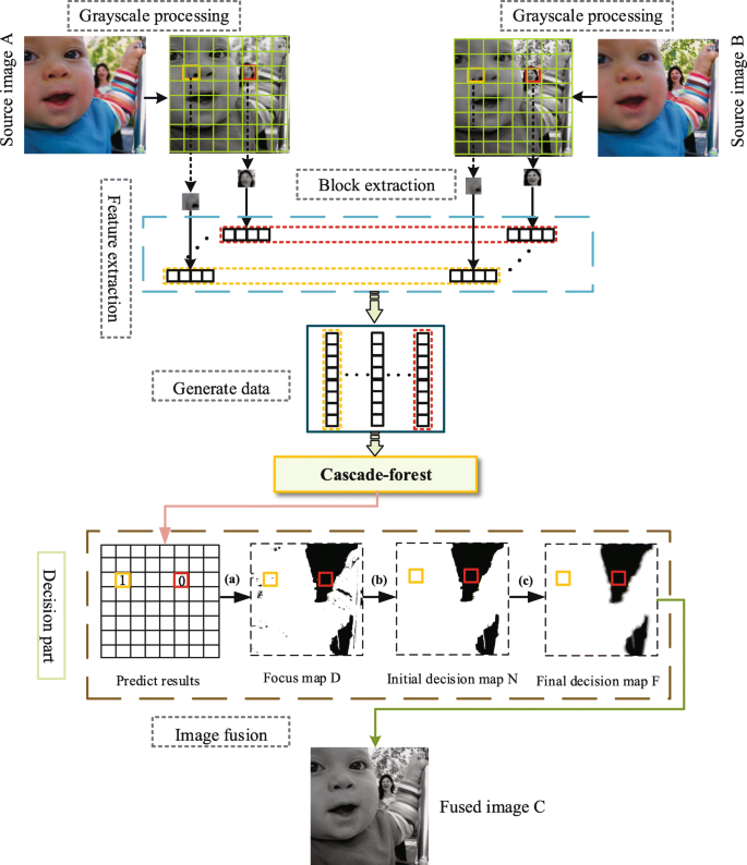
The schematic drawing of the cascade-forest-based method. a Utilize the predict results to generate the focus map. b Remove noise area less than a certain threshold. c Guide image filtering
- 2.
Utilizing the predict results to obtain the focus map
- 3.
Consistency check
- 4.
Guided filtering to acquire the final decision map
- 5.
Generating the fused image through pixel-wise weighted average strategy

3.1 Cascade-forest model design and train
In this paper, image fusion with two source images is considered [31]. Image fusion with more than two images can be discussed separately. As mentioned before, we regard the production of the focus map as a two-class classification topic. As shown in Fig. 3, for each training image, we convert it into gray-scale space. Then, we perform Gaussian filtering on it to obtain its blurred version. Therefore, we acquire the first level of blurred images from the original images. To obtain a variety of relative blurred images, we need to perform multiple levels of Gaussian filtering on the images. In this paper, five different levels of Gaussian filtering are employed to obtain images with distinct blurring levels. We set the standard deviation of the Gaussian filter to 2, and the size of the window is set to 7×7. The current level blurred images are obtained from the previous level blurred images. Hereafter, both original and blurred images are divided into patches following a certain step. Some image patches with less information are discarded (e.g., the variance is less than zero). Then, suitable features are extracted from image patches. The clarity of images is a vital indicator of image quality, and it corresponds to the subjective experience of the people. The extracted four features are Visibility (VIS), Spatial Frequency (SF), Energy of Gradient (EOG), and Variance (VAR). The result of VIS is the difference between intensity of patch pixels and average intensity of an image patch, and intensity represents the pixel value, which can be expressed as
where \(IM\in \mathbb {R}^{J\times L}\) is an image patch, μIM is the average intensity of IM, IM(j,i) indicates the pixel value of the corresponding position, J and L represent the rows and columns of the image patch, respectively, and SF describes the changing characteristics on the image value in space. The higher of the spatial frequency, the clearer of the image patch. It can be defined as
where
Here, SF includes the row frequency and column frequency of image patches. Thence, RF indicates row frequency while CF indicates column frequency. EOG is applied to detect the focal settings of images. The formula is described as
The smaller the gradient energy is, the more blurred the patch is. VAR as an evaluation function to measure the gray level contrast of image patches
where μIM denotes the average gray value of image patches. The clearer the image is, the smaller the function value is.
Patches from source images after feature extraction are assembled, what the cascade-forest does is determining whether patches are relatively clear or relatively blurred. More specifically, for each image patch, Pa and Pb represent the feature vector that after feature extraction. Pa belongs to source image A while Pb belongs to source image B. For example, Pa =(fa1,fa2,fa3,fa4) and Pb =(fb1,fb2,fb3,fb4). When Pa is clearer than Pb, the training sample {Pa,Pb} is set to 1 as a positive sample. In contrast, the training sample {Pa,Pb} is set to 0 as a negative sample when Pb is clearer than Pa. In the training model phase, we select 56 high-quality original images, including all-in-focus and non-all-in-focus. Similar task like [25], it applies 50,000 images from the ImageNet dataset (http://www.image-net.org/). The augment of training data increases the time cost of model training and complicate the training skills of the model. We take the above factor into account and the Cascade-forest can tackle with this issue well. In the end, the training set consists of 250,000 samples that including positive and negative samples. For excellent machine learning models, the validation set is indispensable, and it is the most effective data set to adjust the model. In this paper, we use 15 high-quality images as a validation set, which are fed into the model after the same processing of the training images. There are about 50,000 positive samples and negative samples of the validation set. We have set up four different classifiers as mentioned above. Especially, three classifiers are employed as an ensemble learning method. XGBoost, random forest, and completely random forest are all set to 10 trees, then each tree is grown completely [27]. For reducing the risk of over-fitting, we use fivefold cross-validation to generate the class vector. As for the accuracy of classification, the number of cascaded layers is automatically determined resulting in a completed model.
3.2 Image fusion scheme
3.2.1 Generate focus map
As described in the previous sections, Ia and Ib are respectively considered as two source images with different focus settings. In our method, source images are transformed into gray images when source images are color images. Refining \(\hat {I}_{a}\) and \(\hat {I}_{b}\) as the gray images of Ia and Ib, respectively. Afterwards, \(\hat {I}_{a}\) and \(\hat {I}_{b}\) are segmented into 16×16 image patches. At this stage, overlapped image patches follow the step size of 1. Patches from \(\hat {I}_{a}\) and \(\hat {I}_{b}\) after feature extraction are grouped, and then, they are fed into the pre-trained the cascade-forest model to obtain the classification results of focused and non-focused. The labels of the classification results are 0 or 1. To acquire the focus map, we assign the classification results which represent the focused or non-focused information to all the pixels in the corresponding patches. Figure 4 a shows the focus map that we obtained. As can be seen, when the patches that from image \(\hat {I}_{a}\) is clearer than the patches from image \(\hat {I}_{b}\), pixels of the focus map is set to 1 (white). In contrast, pixels of the focus map are set to 0 (black). As we can see from Fig. 4 a, the focused and non-focused information is accurately distinguished.

Diagrammatic sketch of image fusion process. First, we utilize consistency check to remove noise area of focus map D. Then, guide image filtering is used refine the initial decision map N. Finally, the fused image C is obtained through the pixel-wise processing
3.2.2 Consistency check
Figure 4 a shows the focus map before de-noising. The focus map D is generated with some misclassified pixels, which can be considered as noise. We need to restore and correct these misclassified pixels. In our paper, we reverse these misclassified pixels through removing small areas. In detail, when the noise area is less than the area threshold (0.01×h×w) that we set, we should reverse it (0 changed to 1, 1 changed to 0). In source images, h and w indicate the height and width, respectively. The initial decision map N is shown in Fig. 4 b after removing small areas. As one can see, the decision map becomes more accurate because of the reduced noise area.
3.2.3 Refine the decision map
To reduce undesirable artifacts around the boundaries between the focused and non-focused regions, we use the GF to refine the initial decision map N. The GF has excellent characteristics of edge-reservation. As shown in the following equations.
where GuidedFilter(·) represents the guided filtering. The local box radius w and regularization parameter ε as the two parameters for guided image filter are set to 8 and 0.1, respectively. Figure 4 c illustrates the final decision map F.
3.2.4 Fusion
The final fused image is presented in Fig. 4 d. At last, when we acquire the final decision map F, the fused result C is obtained through the pixel-wise processing principle
where A and B represent source image A and source image B, respectively.
4 Results and discussion
To test the performance of the proposed fusion method, we apply 21 pairs of multi-focus images as test images. As Fig. 5 exhibited, these are a portion of test images. To ensure that test results are fair and comprehensive, test images include some traditional multi-focus images and some images from dataset “Lytro (http://mansournejati.ece.iut.ac.ir/content/lytro-multi-focus-dataset).” Figure 6 shows the intermediate results of six pairs test images in our method.

A part of test images of the proposed method. We show some test images that are taken from different dataset

Intermediate fusion results of portion test images in our method. For each test image, we convert it into gray-scale space. Then, intermediate results of image fusion process are present. The effect of focus map and decision map are significant
We enumerate six representative fusion methods, including spatial domain methods and transform domain methods. They are the CNN [25], GFF [19], SR [16], NSCT [15], NSCT-SR [32], and CVT-based method [33]. All methods involved in the above comparison are applying default parameters associated with corresponding papers.
Results of image fusion are mainly evaluated according to subjective visual and objective metrics. Due to the details about images are difficult to be captured by personal visual, objective evaluation is particularly significant in image fusion. In our paper, we have adopted four objective evaluation metrics, which are MI [34], QAB/F [35], FMI [36], and SD. MI represents the normalized mutual information. QAB/F represents the reserved value of edge information. FMI represents the feature mutual information. SD represents standard deviation. As regards to the above four evaluation metrics, higher value indicates the better performance.
4.1 Comparison studies
To verify the validity of the proposed method, we demonstrate visual comparisons and quantitative comparisons of different multi-focus fusion methods. Therefore, three pairs of test images were randomly selected from test images as examples to show the difference between our method and others.
As shown in Fig. 7, different fusion results of “Disk” source images are presented. The border area of each fused image between focused and non-focused is displayed in the upper left corner to clearly distinguish the difference. Figure 7 c–f generates some improper artifacts at the boundary of the clock, especially the CVT-based method. As we can see from the magnification area that the boundary region of the clock has an unnatural effect. These artifacts cause a negative impact on the quality of the fused images. Figure 7 g obtained from the GF-based method is blurred on the boundary region as well. Afterward, the CNN-based method obtained Fig. 7 h with the favorable overall effect. However, there is no denying that the details were not handled well. Figure 7 i shows the result obtained from our method. It can be observed that the result of our method provides better performance in terms of visual effects. Table 1 shows quantitative comparisons of distinct methods of image “Disk.” It can be further verified from the four evaluation metrics that our method has a relatively outstanding performance.

Fusion results of “Disk” source images. Fusion results of different methods of “Disk” source images are presented. The border area of each fused image between focused and non-focused is displayed in the lower left corner to clearly distinguish the difference. Intermediate fusion results of our methods are shown as focus map and decision map
Figure 8 shows subjective comparisons of the fused results obtained from distinct image fusion methods. Then, Table 2 presents the corresponding quantitative comparisons. Magnified regions show distinctive details. The fused images of Fig. 8 d–f are more ambiguous on the fusion boundary of the magnified region. Figure 8 c as the result of the SR-based method, the image quality is much better, it still has some artifacts in the fusion boundary region. Figure 8 g and h are visually well enough. However, the lack of details of source images results in insufficient image quality. Figure 8 i represents our method, which achieves the fusion result with high reliability and superior performance. Table 2 shows that our method has the highest objective evaluation as compared to other methods.

Fused results of “Toy” source images. Fusion results of different methods of “Toy” source images are presented. The border area of each fused image between focused and non-focused is displayed in the lower left corner to clearly distinguish the difference. Intermediate fusion results of our methods are shown as focus map and decision map
Besides, Fig. 9 displays the subjective results of the “Profile,” the magnification area is extracted from each image. It can be seen that Fig. 9 d with inferior quality. Figure 9 f reduces the artifacts generated with Fig. 9 e and obtained better image quality. Figure 9 c puts up a more excellent performance. Figure 9 g and h present the fused images obtained from the GFF-based method and the CNN-based method, respectively. Although Fig. 9 g and h show more outstanding performance than those of previous fusion methods, the fusion area of the “nos” still failed to achieve the desired effect. However, Fig. 9 g obtained by our method shows a prominent performance. The edge in the image is better preserved, and the details of source images are transmitted to the fused result. According to the data of Table 3, the proposed method has better objective evaluation. The CVT-based methods as a traditional method requires more improvements. The NSCT-SR-based methods overcomes the shortcoming of the NSCT-based methods and obtains a better objective evaluation. The objective evaluation of the SR-based methods and the GFF-based methods is better than that mentioned above. Afterwards, CNN-based methods with an innovative thought achieves excellent performance. In contrast, the objective evaluation of our method is the highest in terms of four metrics.

Fusion results of “Profile” source images. Fusion results of different methods of “Profile” source images are presented. The border area of each fused image between focused and non-focused is displayed in the upper left corner to clearly distinguish the difference. Intermediate fusion results of our methods are shown as focus map and decision map
4.2 Parameters comparison of the proposed method
Fusion methods which adopt different parameters setting will inevitably result in fused images with distinctive performance. First of all, different steps of overlapping extract blocks can affect the results of the proposed method. It is known that too-large step will have a block effect on image fusion. As it is shown in Fig. 10 a–c, we can perceive that when the step is 2 or step is 3, the focus map has a manifest block effect. The blocking effect has a negative impact on the performance of the image. Figure 10 d–f shows the results, acquired by utilizing different steps, that the area within the fusion boundary is enlarged and placed in the lower-left corner. Table 4 shows the average of the evaluation indicators for 21 test images with different steps. When the step size is 1, the fused image without block effect has the best performance.

Influence of distinct steps on fused images. Number represents the step sizes. Different steps of overlapping extract blocks will be affecting the results of the proposed method
As [25] elaborated, the size of the image block corresponds to the amount of information contained. However, if we assign the image patches size too large, image patches are usually not accurate enough. The larger size tends to comprise both focused and non-focused regions. On the contrary, when the size of the patch is set too small, patches may not guarantee the accuracy of the classification. Besides, it also greatly increases the time cost of the experiments. Based on the above discussions, we verify with 21 test images. As shown in Fig. 11, the performance of the proposed method follows the changes of image patch size. Nevertheless, there is no significant increase or decrease in each evaluation metric. It indicates our method is insensitive to the size of the image patch.

The influence of patch size on four metrics. The size of the image block corresponds to the amount of information contained. Too-large patch sizes are usually resulting in inaccurate classification. Too-small patch sizes increase the time cost of the experiments. We obtained the optimal parameters by verifying different patch sizes
5 Conclusions
In this paper, we propose an efficient multi-focus image fusion method for improving imaging systems. Considering the influence of fusion rules, we introduce the cascade-forest into multi-focus image fusion. And we adopt effective activity level measurement. Activity level measurement and fusion rule represent feature extraction and classification algorithm, respectively. To improve the model, not only are four effective features extracted, but also four excellent algorithms are integrated. Artifacts are eliminated by considering the boundaries between the focused and non-focused regions. Through analyzing and comparing, the validity of the suggested method is verified.
Availability of data and materials
Please contact author for data requests.
Abbreviations
- ANN:
-
Artifcial neural network
- CART:
-
Classifcation and regression trees
- CNN:
-
Convolutional neural network
- CVT:
-
Curvelet
- DL:
-
Deep learning
- DNN:
-
Deep neural networks
- DOF:
-
Depth-of-field
- DTCWT:
-
Dual-tree complex wavelet transform
- DWT:
-
Discrete wavelet transform
- EOF:
-
Energy Of gradient
- GF:
-
Guided filter
- GP:
-
The gradient pyramid
- LP:
-
Laplacian pyramid
- ML:
-
Machine learning
- MP:
-
Morphological pyramid
- MST:
-
Multi-scale transform
- NSCT:
-
Nonsubsampled contourlet transform
- RGF:
-
Rolling guidance filter
- SF:
-
Spatial frequency
- SR:
-
Sparse representation
- SVM:
-
Support vector machine
- VAR:
-
Variance
- VIS:
-
Visibility
- WA:
-
Weighted average
- WT:
-
Wavelet transform
- XGBoost:
-
Extreme gradient boosting
References
K. L. Naga Kishore, A. V. Vinod Kumar, N. Nagaraju, in International Research Journal of Engineering and Technology (IRJET). An effective multi-focus medical image fusion using dual tree compactly supported shear-let transform based on local energy means, (2016), pp. 53–61.
Y. K. S. Kumar, Sandeep, M. Bhattacharya, in Proceedings of the International Conference on Image Processing, Computer Vision, and Pattern Recognition (IPCV). Curvelet based multi-focus medical image fusion technique: Comparative study with wavelet based approach, (2011), p. 03.
X. Dai, H. Zhang, T. Liu, H. Shu, L. Luo, Legendre moment invariants to blur and affine transformation and their use in image recognition. Pattern. Anal. Applic.17(2), 311–326 (2014).
H. Zhu, M. Liu, H. Ji, Y. Li, Combined invariants to blur and rotation using zernike moment descriptors. Pattern. Anal. Applic.13(3), 309–319 (2010).
T. Stathaki, Image Fusion: Algorithms and Applications (Academic Press, 2008).
Z. Zhang, R. S. Blum, in Proceedings of the IEEE. A categorization and study of multiscale-decomposition-based image fusion schemes, (1999), pp. 671–679. https://doi.org/10.1109/5.775414.
P. J. Burt, E. H. Adelson, in Readings in Computer Vision. The laplacian pyramid as a compact image code (Elsevier, 1987), pp. 671–679. https://doi.org/10.1016/b978-0-08-051581-6.50065-9.
W. Wang, F. Chang, A multi-focus image fusion method based on laplacian pyramid. J. Comput.6(12), 2559–2566 (2011).
V. S. Petrovic, C. S. Xydeas, Gradient-Based Multiresolution Image Fusion (IEEE Press, 2004). https://doi.org/10.1109/tip.2004.823821.
A. Toet, A morphological pyramidal image decomposition. Pattern Recogn. Lett.9(4), 255–261 (1989).
D. A. Godse, D. S. Bormane, 3. Wavelet based image fusion using pixel based maximum selection rule, (2011), pp. 63–72.
H. Wang, J. Peng, W. Wu, Fusion algorithm for multisensor images based on discrete multiwavelet transform. IEE Proc. Vis. Image Signal Process.149(5), 283–289 (2002).
H. Li, B. S. Manjunath, S. K. Mitra, in Image Processing, 1994. Proceedings. ICIP-94., IEEE International Conference. Multisensor image fusion using the wavelet transform, (2002), pp. 235–245. https://doi.org/10.1006/gmip.1995.1022.
J. J. Lewis, R. J. O’Callaghan, S. G. Nikolov, D. R. Bull, N. Canagarajah, Pixel- and region-based image fusion with complex wavelets. Inf. Fusion. 8(2), 119–130 (2007).
Q. Zhang, B. L. Guo, Multifocus image fusion using the nonsubsampled contourlet transform. Signal Process.89(7), 1334–1346 (2009).
B. Yang, S. Li, Multifocus image fusion and restoration with sparse representation. IEEE Transactions on Instrumentation and Measurement. 59(4), 884–892 (2010).
Q. Li, X. Yang, W. Wu, K. Liu, G. Jeon, Multi-focus image fusion method for vision sensor systems via dictionary learning with guided filter. Sensors. 18(7), 84–92 (2018).
A. Chianese, F. Marulli, V. Moscato, F. Piccialli, in Indoor Positioning and Indoor Navigation (IPIN), 2013 International Conference On. A “smart” multimedia guide for indoor contextual navigation in cultural heritage applications, (2013), pp. 1–6. https://doi.org/10.1109/ipin.2013.6851448.
S. Li, X. Kang, J. Hu, Image fusion with guided filtering. IEEE Trans. Image Process.22(7), 2864–2875 (2013).
L. Jian, X. Yang, Z. Zhou, K. Zhou, K. Liu, Multi-scale image fusion through rolling guidance filter. Futur. Gener. Comput. Syst.83:, 310–325 (2018).
S. Li, J. T. Kwok, Y. Wang, Multifocus image fusion using artificial neural networks. Pattern Recogn. Lett.23(8), 985–997 (2002).
I. De, B. Chanda, Multi-focus image fusion using a morphology-based focus measure in a quad-tree structure. Inf. Fusion. 14(2), 136–146 (2013).
X. Bai, Y. Zhang, F. Zhou, B. Xue, Quadtree-based multi-focus image fusion using a weighted focus-measure. Inf. Fusion. 22:, 105–118 (2015).
G. Mamatha, S. A. Rahim, C. P. Raj, Feature-level multi-focus image fusion using neural network and image enhancement. Glob. J. Comput. Sci. Technol. (2012).
Y. Liu, X. Chen, H. Peng, Z. Wang, Multi-focus image fusion with a deep convolutional neural network. Inf. Fusion. 36:, 191–207 (2017).
W. Wu, X. Yang, Y. Pang, J. Peng, G. Jeon, A multifocus image fusion method by using hidden markov model. Opt. Commun.287:, 63–72 (2013).
Z. -H. Zhou, J. Feng, Deep forest: Towards an alternative to deep neural networks. arXiv preprint arXiv:1702.08835 (2017).
T. Chen, C. Guestrin, in ACM SIGKDD International Conference on Knowledge Discovery and Data Mining. Xgboost: A scalable tree boosting system, (2016), pp. 785–794. https://doi.org/10.1145/2939672.2939785.
K. He, J. Sun, X. Tang, in European Conference on Computer Vision. Guided image filtering (Springer, 2010), pp. 1–14.
Y. Chai, X. Cao, in 2018 IEEE 3rd Advanced Information Technology, Electronic and Automation Control Conference (IAEAC). Stereo matching algorithm based on joint matching cost and adaptive window (IEEE, 2018), pp. 442–446. https://doi.org/10.1109/iaeac.2018.8577495.
W. Zhao, D. Wang, H. Lu, in IEEE Transactions on Circuits and Systems for Video Technology. Multi-focus image fusion with a natural enhancement via joint multi-level deeply supervised convolutional neural network, (2018). https://doi.org/10.1109/tcsvt.2018.2821177.
Y. Liu, S. Liu, Z. Wang, A general framework for image fusion based on multi-scale transform and sparse representation. Inf. Fusion. 24:, 147–164 (2015).
L. Tessens, A. Ledda, A. Pizurica, W. Philips, in Acoustics, 2007. ICASSP 2007. Proceedings of the IEEE International Conference on Acoustics, Speech, and Signal Processing. Extending the depth of field in microscopy through curvelet-based frequency-adaptive image fusion (IEEE, 2007). https://doi.org/10.1109/icassp.2007.366044.
M. Hossny, S. Nahavandi, D. Creighton, Comments on information measure for performance of image fusion. Electron. Lett.44(18), 1066–1067 (2008).
C. Xydeas, V. Petrovic, Objective image fusion performance measure. Electron. Lett.36(4), 308–309 (2000).
M. B. A. Haghighat, A. Aghagolzadeh, H. Seyedarabi, A non-reference image fusion metric based on mutual information of image features. Comput. Electr. Eng.37(5), 744–756 (2011).
Acknowledgments
Thanks to all those who have suggested and given guidance for this article.
Funding
The research in our paper is sponsored by National Natural Science Foundation of China (no. 61701327), China Postdoctoral Science Foundation (no. 2018M640916), Science Foundation of Sichuan Science and Technology Department (no. 2018GZ0178), Fujian Provincial Key Laboratory of Information Processing and Intelligent Control (Minjiang University) (no. MJUKF-IPIC201805)
Author information
Authors and Affiliations
Contributions
All the authors of this article contributed to this article. LH carried out the design and summary of the study. XMY, LL, WW, AA, and GJ participated in the experimental design and results analysis and helped write the manuscript. All authors read and approved the final manuscript.
Corresponding author
Ethics declarations
Competing interests
The authors declare that they have no competing interests.
Additional information
Publisher’s Note
Springer Nature remains neutral with regard to jurisdictional claims in published maps and institutional affiliations.
Rights and permissions
Open Access This article is distributed under the terms of the Creative Commons Attribution 4.0 International License (http://creativecommons.org/licenses/by/4.0/), which permits unrestricted use, distribution, and reproduction in any medium, provided you give appropriate credit to the original author(s) and the source, provide a link to the Creative Commons license, and indicate if changes were made.
About this article

Cite this article
He, L., Yang, X., Lu, L. et al. A novel multi-focus image fusion method for improving imaging systems by using cascade-forest model. J Image Video Proc. 2020, 5 (2020). https://doi.org/10.1186/s13640-020-0494-8
Received:
Accepted:
Published:
DOI: https://doi.org/10.1186/s13640-020-0494-8