


1 Introduction
Interactions between planar shock waves of opposite families (i.e., deflecting the free stream flow in opposite directions) have been a topic of interest in the field of gas dynamics for past decades (Ben-Dor Reference Ben-Dor2007). It is well known that, for a range of flow conditions, these shock interactions form a bi-stable system for which either the regular interaction (RI) or the Mach interaction (MI) materialise. The former, depicted in figure 1(a), involves five discontinuities: two incident shock waves  $C_{1}$ and
  $C_{2}$, two reflected shock waves
  $C_{3}$ and
  $C_{4}$, and a slipline
  $s$. Following the work of Edney (Reference Edney1968), the RI is classified as a type I interference. The compatibility condition for this interaction pattern involves equal static pressure and flow direction in regions (3) and (4), whilst other flow properties differ (only in the particular case of a symmetric interaction both states (3) and (4) are identical and no slipline exists). In the event of an MI, in turn, incident shock waves
  $C_{1}$ and
  $C_{2}$ no longer intersect due to a quasi-normal shock segment appearing in the flow. This wave pattern is classified as a type II interference (Edney Reference Edney1968). Schematics of the MI are included in figure 1(b), in which the quasi-normal shock segment, commonly known as the Mach stem, is labelled as
  $m$. Its presence entails two sliplines
  $s_{1}$ and
  $s_{2}$ that enclose the non-homogeneous region (5) of subsonic flow. A necessary stability requirement is that the slipline pair forms a virtual convergent duct, which allows the subsonic flow in (5) to accelerate. However, this requirement is not sufficient; the presence of (at least) one Prandtl–Meyer expansion fan (PME) is paramount to establish a virtual throat and a divergent duct segment between the slipline pair to enable the enclosed flow to reach supersonic velocities. The resulting Mach stem height is such that all the mass flow through it passes through the virtual slipline throat at sonic conditions. As opposed to the RI, the Mach stem height as well as the spatial extent of the MI are thus linked to a characteristic length scale that relates the incident shock foot locations with the origin of the PME(s) (Hornung & Robinson Reference Hornung and Robinson1982; Li & Ben-Dor Reference Li and Ben-Dor1997; Mouton & Hornung Reference Mouton and Hornung2007; Tao et al. Reference Tao, Liu, Fan, Xiong, Yu and Sun2017).

Figure 1. Schematic of (a) the regular interaction, (b) the Mach interaction and (c) shock polar representation in the pressure-deflection plane for  $M_{\infty }=3$. Here,
  $\unicode[STIX]{x1D717}_{2}^{r}$ and
  $\unicode[STIX]{x1D717}_{2}^{m}$ indicate a general solution outside the dual-solution domain for the regular and the Mach interaction, whilst flow states within the dual-solution domain are highlighted in blue for the former and red for the latter. Sonic conditions in (c) are labelled with an
  $\times$.
It is common practice to use shock polar theory to establish steady-state stability boundaries between the RI and the MI in the parameter space (Li, Chpoun & Ben-Dor Reference Li, Chpoun and Ben-Dor1999). A typical shock polar representation in the pressure-deflection plane is included in figure 1(c) for free stream Mach number  $M_{\infty }=3$, specific heat ratio
  $\unicode[STIX]{x1D6FE}=1.4$ and upper flow deflection
  $\unicode[STIX]{x1D717}_{1}=25^{\circ }$. Here, the detachment condition
  $\unicode[STIX]{x1D717}_{2}^{d}$ denotes the maximum flow deflection imposed by
  $C_{2}$ for which the polars
  $r_{1}$ and
  $r_{2}$ intersect (in this limit case, they are tangent). Beyond this value, there is no longer an RI configuration capable of providing compatible states (3) and (4), and so the MI materialises. On the contrary, the von Neumann criterion
  $\unicode[STIX]{x1D717}_{2}^{n}$ defines a lower flow deflection for which the three polars,
  $i$,
$i$,  $r_{1}$ and
  $r_{2}$, intersect at one location. Further reducing
  $\unicode[STIX]{x1D717}_{2}$ prevents the slipline pair
  $s_{1}$–
 $s_{2}$ from being convergent, which impedes the formation of a stable MI and thus the RI solution prevails thereafter. It is interesting to note that at von Neumann both RI and MI provide identical flow states (3) and (4) and therefore they would be in mechanical equilibrium at this condition. Another feature in figure 1(c) is the occurrence of a dual-solution domain (DSD), shaded in light grey and spanning between
  $\unicode[STIX]{x1D717}_{2}^{n}\leqslant \unicode[STIX]{x1D717}_{2}\leqslant \unicode[STIX]{x1D717}_{2}^{d}$, for which the two solutions, RI and MI, are both physically possible. As first hypothesised by Hornung, Oertel & Sandeman (Reference Hornung, Oertel and Sandeman1979), this allows for a potential flow hysteresis, that is, the solution that materialises and the RI
 $\rightleftarrows$MI transition conditions can depend on the flow history.
Asymmetric shock interactions are present in a wide range of high speed aerodynamics applications (Li et al. Reference Li, Chpoun and Ben-Dor1999; Délery & Dussauge Reference Délery and Dussauge2009). Supersonic inlets are a clear example, comprising a set of oblique shock waves that compress the flow to suitable pressures for combustion. Avoiding  $\text{RI}\rightarrow \text{MI}$ transition is of paramount importance due to the associated entropy rise, total pressure loss and high risk of engine unstart. Even though steady flow theory provides useful insight on the shock pattern developing inside the inlet, it fails at predicting the premature
  $\text{RI}\rightarrow \text{MI}$ transition observed when disturbances are present in the free stream flow (Hornung & Robinson Reference Hornung and Robinson1982; Chpoun et al. Reference Chpoun, Passerel, Li and Ben-Dor1995; Ivanov, Khotyanovsky & Nikiforov Reference Ivanov, Khotyanovsky, Kudryavtsev and Nikiforov2001) eventually preventing the occurrence of any flow hysteresis. On these grounds, only low-noise wind tunnel conditions (Ivanov et al. Reference Ivanov, Kudryavtsev, Nikiforov, Khotyanovsky and Pavlov2003) and disturbance-free numerical computations (Chpoun & Ben-Dor Reference Chpoun and Ben-Dor1995; Ivanov, Gimelshein & Beylich Reference Ivanov, Gimelshein and Beylich1995; Vuillon, Zeitoun & Ben-Dor Reference Vuillon, Zeitoun and Ben-Dor1995; Ivanov et al. Reference Ivanov, Ben-Dor, Elperin, Kudryavtsev and Khotyanovsky2002) permitted the penetration of the RI inside the steady-state DSD in agreement with theoretical predictions.
A specific class of flow phenomena involving asymmetric shock interactions is the reflection of a shock wave at a wall with a turbulent boundary layer, the so called shock-wave/turbulent-boundary-layer interaction (SWTBLI), also present in supersonic intakes and nozzle flows (Babinsky & Harvey Reference Babinsky and Harvey2011). If the adverse pressure gradient imposed by the shock is strong enough to cause boundary layer separation, the location and strength of the separation shock becomes highly unsteady and so does its interaction with the incident shock (Délery & Dussauge Reference Délery and Dussauge2009; Touber & Sandham Reference Touber and Sandham2011). Recent large-eddy simulations (LES) of SWTBLI performed by Matheis & Hickel (Reference Matheis and Hickel2015) at a free stream Mach number  $M_{\infty }=2$ demonstrate that such unsteadiness may cause premature
  $\text{RI}\rightarrow \text{MI}$ transition and sustain the MI pattern for mean flow conditions beyond its steady-state stability boundary. This clearly highlights the potential impact of flow disturbances in the shock interaction topology. Previous fundamental research on disturbed shock interactions has been limited to the effect of impulsive disturbances on symmetric shock systems, mainly either in the form of incoming velocity perturbations (Ivanov et al. Reference Ivanov, Markelov, Kudryavtsev and Gimelshein1998), shocks, expansion waves and contact discontinuities in the free stream (Kudryavtsev et al. Reference Kudryavtsev, Khotyanovsky, Ivanov, Hadjadj and Vandromme2002), laser pulses (Khotyanovsky, Kudryavtsev & Ivanov Reference Khotyanovsky, Kudryavtsev and Ivanov2006), dense particles (Mouton & Hornung Reference Mouton and Hornung2008), water vapour (Sudani et al. Reference Sudani, Sato, Karasawa, Noda, Tate and Watanabe2002) or impulsive wedge rotation (Markelov, Pivkin & Ivanov Reference Markelov, Pivkin and Ivanov1999; Felthun & Skews Reference Felthun and Skews2004; Naidoo & Skews Reference Naidoo and Skews2011). However, practically relevant scenarios involving asymmetric shock structures perturbed in a continuous manner (i.e., representative for unsteady internal flows) remain to date still unexplored.

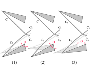
Figure 2. Unsteady effects on the incident shock  $C_{2}$ for the lower wedge excitation mechanisms considered: (a) pitch, (b) periodic deflection oscillation and (c) periodic streamwise oscillation.
In the present paper we therefore conduct a set of inviscid computations with the purpose of providing insight on the dynamics of unsteady asymmetric shock interactions affected by a continuous excitation. Two wedges are used to asymmetrically deflect the free stream flow and introduce the incident shock waves and two centred PME in the computational domain. After a steady state is reached, the shock system is excited according to three different excitation scenarios depicted, respectively, in figure 2(a–c): pitching of the lower wedge across the steady-state DSD, a periodic (sinusoidal) oscillation of the lower wedge deflection around a mean value both within and outside of the steady-state DSD, and a periodic (sinusoidal) streamwise oscillation of the lower wedge without pitch. The response of the system is analysed with a strong focus on the bi-directional RI $\rightleftarrows$MI transition process and the underlying mechanism by which the MI is found to be more robust than the RI under flow perturbations.
The paper is organised as follows: in § 2 we describe our computational set-up, the numerical model and the post-processing algorithm developed for the transient analysis, and we assess the grid dependency of the computations. In § 3 we present the results of our numerical simulations conducted at  $M_{\infty }=3$ and
  $\unicode[STIX]{x1D717}_{1}=25^{\circ }$, hereafter referred to as the baseline conditions. Results for the lower wedge pitch are discussed in § 3.1 along with a shock polar analysis in the shock frame of reference for the
  $\text{RI}\rightarrow \text{MI}$ transition. In turn, §§ 3.2 and 3.3 are focused on the periodic oscillation of the lower wedge deflection and lower wedge streamwise location, respectively. The paper is finally concluded in § 4 along with further remarks.

Figure 3. Schematic diagram of the computational domain.
2 Computational set-up
2.1 Problem definition
A sketch of the investigated computational domain is given in figure 3. We consider two wedges of equal hypotenuse  $w$ asymmetrically deflecting the free stream flow at Mach
  $M_{\infty }=3$ and generating a pair of intersecting waves
  $C_{1}$,
  $C_{2}$ and centred PME. The wedges are not included in the computational domain, however. Instead, we account for their effect through time dependent boundary conditions satisfying the Rankine–Hugoniot relations across the incident shocks
  $C_{1}~((0)\rightarrow (1))$ and
  $C_{2}~((0)\rightarrow (2))$, and Prandtl–Meyer expansion theory for the PME in (3) and (4). Note that since each trailing edge, and thus the PME origins, is placed on top of an horizontal domain boundary, states (3) and (4) relate to flow conditions along horizontal expansion rays. Concerning shock generator geometry, one characteristic length scale is the wedge hypotenuse
  $w$, which is set to
  $w=1$ for all computations. However, the resulting wave system is most sensitive to the geometrical ratio of vertical wedge separation distance (
 $2g$) to wedge hypotenuse,
  $2g/w$. This parameter determines whether or not reflected shocks
  $C_{3}$ and
  $C_{4}$ impinge on the wedges, and thus potentially leading to domain unstart, but also imposes a relation between incident shock foot locations and the origin of the centred PME. As already mentioned, this influences the spatial extent and the steady-state Mach stem height of the MI configuration. Unless otherwise stated,
  $2g/w$ is set to 0.84 as commonly used in the literature (Ivanov et al. Reference Ivanov, Ben-Dor, Elperin, Kudryavtsev and Khotyanovsky2002; Kudryavtsev et al. Reference Kudryavtsev, Khotyanovsky, Ivanov, Hadjadj and Vandromme2002). Rotation and oscillation of the lower wedge deflection occur around point O as indicated in figure 2(a–c), and, except for the streamwise oscillation, both wedge trailing edges are positioned at the same
  $x$ location (
 $x_{ut}=x_{lt}$ in figure 3). Lastly, the upstream length of the domain,
  $L_{1}=w$, establishes free stream (0) conditions at the left boundary throughout the computations, and
  $L_{2}=1.4w$ ensures that the flow at the outlet (5) is always supersonic.
2.2 Numerical method
We solve the two-dimensional unsteady Euler equations in conservative form
 $$\begin{eqnarray}\frac{\unicode[STIX]{x2202}\boldsymbol{U}}{\unicode[STIX]{x2202}t}+\frac{\unicode[STIX]{x2202}\boldsymbol{F}}{\unicode[STIX]{x2202}x}+\frac{\unicode[STIX]{x2202}\boldsymbol{G}}{\unicode[STIX]{x2202}y}=0,\end{eqnarray}$$
where
 $$\begin{eqnarray}\boldsymbol{U}=\left[\begin{array}{@{}c@{}}\unicode[STIX]{x1D70C}\\ \unicode[STIX]{x1D70C}u\\ \unicode[STIX]{x1D70C}v\\ E\end{array}\right],\quad \boldsymbol{F}=\left[\begin{array}{@{}c@{}}\unicode[STIX]{x1D70C}u\\ \unicode[STIX]{x1D70C}u^{2}+p\\ \unicode[STIX]{x1D70C}uv\\ u(E+p)\end{array}\right],\quad \boldsymbol{G}=\left[\begin{array}{@{}c@{}}\unicode[STIX]{x1D70C}v\\ \unicode[STIX]{x1D70C}uv\\ \unicode[STIX]{x1D70C}v^{2}+p\\ v(E+p)\end{array}\right].\end{eqnarray}$$
 The equations are non-dimensionalised using the free stream velocity  $u_{\infty }$ and the wedge hypotenuse
  $w$, which combined define the characteristic time scale
  $w/u_{\infty }$ of the problem. To close the system, the equation of state for a perfect gas is used
 $$\begin{eqnarray}p=(\unicode[STIX]{x1D6FE}-1)\left(E-\unicode[STIX]{x1D70C}\frac{u^{2}+v^{2}}{2}\right),\end{eqnarray}$$
 with the specific heat ratio  $\unicode[STIX]{x1D6FE}=1.4$. The system of governing equations is discretised on a Cartesian grid with a conservative finite volume scheme. The in-house solver INCA has been used for the computations (Hickel, Egerer & Larsson Reference Hickel, Egerer and Larsson2014). Fluxes are computed first at the cell centres, then projected into the right eigenvector space where a local Lax–Friedrichs flux vector splitting and a third-order weighted essentially non-oscillatory (WENO) reconstruction of the flux through the cell face is performed, and finally they are projected back to the conserved quantities (Shu Reference Shu1998). A third-order explicit Runge–Kutta scheme is used for time integration; see Hickel et al. (Reference Hickel, Egerer and Larsson2014) for implementation details.
2.3 Post-processing
For rapid excitations, unsteady effects manifest and the instantaneous lower wedge deflection is no longer representative of the flow deflection  $\unicode[STIX]{x1D717}_{2}$ across
  $C_{2}$ near the interaction point (i.e.,
  $C_{2}$ is curved, see figure 2). Thus, to properly characterise transition it is imperative to measure quantities of interest, i.e., lower flow deflection
  $\unicode[STIX]{x1D717}_{2}(t)$, static pressure rise
  $p/p_{\infty }(t)$ and entropy jump
  $\unicode[STIX]{x0394}s(t)$, at the interaction location. A custom post-processing algorithm was developed for this purpose. Incident shock waves
  $C_{1}$ and
  $C_{2}$ are tracked by searching for the local maximum of the density gradient magnitude
  $\sqrt{(\unicode[STIX]{x2202}\unicode[STIX]{x1D70C}/\unicode[STIX]{x2202}x)^{2}+(\unicode[STIX]{x2202}\unicode[STIX]{x1D70C}/\unicode[STIX]{x2202}y)^{2}}$ along each row of the grid starting from the left. Depending on whether the shock topology is an MI, the Mach stem is formed. In that case, a marked entropy jump occurs, see figure 9(a), accompanied by a clear formation of a minimum and a maximum of vorticity at the upper and lower triple point locations, respectively. Subgrid resolution for the location of vorticity extrema is achieved by local parabolic reconstruction. The vertical distance between the resulting points thus defines the instantaneous Mach stem height
  $h_{ms}$; see figure 9(b). Other quantities of interest are determined in their vicinity; e.g, instantaneous
  $\unicode[STIX]{x1D717}_{2}$ measurements are taken at a distance of
  $0.01w$ in the negative
  $y$-direction from the lower triple point, whilst the pressure rise across the wave system
  $p/p_{\infty }$ is recorded
  $0.01w$ downstream of both triple points, respectively. The instantaneous entropy jump
  $\unicode[STIX]{x0394}s$ is defined as
  $s_{i}-s_{\infty }$ where
  $s_{i}$ is measured at
  $0.01w$ downstream of the local Mach stem (over the fictional horizontal line that bisects both triple points) and
  $s_{\infty }$ is the free stream value. Magnitudes are averaged with neighbouring cells to avoid oscillations. In the case of an RI, the entropy jump is small and
  $C_{1}$ and
  $C_{2}$ intersect. This is considered to be the interaction location, and instantaneous
  $\unicode[STIX]{x1D717}_{2}$,
  $p/p_{\infty }$ and
  $\unicode[STIX]{x0394}s$ measurements follow in a similar fashion as explained for the MI case.
2.4 Grid sensitivity
The flow is discretised on a uniform grid with spacing  $h$ in both spatial directions. In order to assess the impact of the grid size on the shock dynamics and the corresponding bi-directional transition process, a grid convergence analysis was performed. For the baseline conditions, both an initial RI and MI were independently considered by setting
  $\unicode[STIX]{x1D717}_{2,0}=12^{\circ }$ and
  $\unicode[STIX]{x1D717}_{2,0}=19^{\circ }$, respectively. After the steady state was reached, transition to the opposite shock pattern was enforced by linearly changing the lower wedge deflection at a constant rate; i.e., increased to enforce
  $\text{RI}\rightarrow \text{MI}$ transition and decreased in the opposite case. Similar to Felthun & Skews (Reference Felthun and Skews2004), the rotational velocity of the wedge is defined in terms of the Mach number of the wedge tip
  $M_{tip}$ divided by the free stream value
  $M_{\infty }$, which is equivalent to the ratio of the wedge tip velocity to free stream velocity. For the grid convergence analysis,
  $M_{tip}/M_{\infty }$ was set to 0.01. The instantaneous lower flow deflection in the vicinity of the interaction was recorded at transition for four different grid spacings:
  $w/h=200,400,800$ and
  $1600$, with the corresponding results shown in figure 4. As observed, a clear flow deflection convergence is obtained for
  $w/h=1600$ regardless of the direction of transition so this value was used for all further computations.

Figure 4. Results of the grid sensitivity study.
3 Results
3.1 Pitch of lower wedge
The first excitation mechanism corresponds to the pitching of the lower wedge across the steady-state DSD. For the baseline conditions ( $M_{\infty }=3$ and
  $\unicode[STIX]{x1D717}_{1}=25^{\circ }$), the steady-state DSD extends from the von Neumann condition
  $\unicode[STIX]{x1D717}_{2}^{n}=14.14^{\circ }$ until detachment at
  $\unicode[STIX]{x1D717}_{2}^{d}=17.43^{\circ }$; see figure 1(c). Both RI and MI are considered as the starting shock topology by setting the initial lower wedge deflection to
  $\unicode[STIX]{x1D717}_{2,0}=12^{\circ }$ for the former and
  $\unicode[STIX]{x1D717}_{2,0}=19^{\circ }$ for the latter. After reaching a converged steady-state solution, the lower wedge deflection is changed at a linear rate to enforce transition; see § 2.4. Rotational velocities corresponding to
  $M_{t}/M_{\infty }=0.1$, 0.01, 0.001 and 0.0001 are considered. A summary of relevant parameters can be found in table 1.

Figure 5. Lower flow deflection  $\unicode[STIX]{x1D717}_{2}$ at transition as a function of the rotational velocity of the lower wedge: (▾, ▿) numerical data for
  $\text{MI}\rightarrow \text{RI}$ transition, (▴) numerical data for
  $\text{RI}\rightarrow \text{MI}$ transition, (●)
  $\text{RI}\rightarrow \text{MI}$ transition predictions based on shock polar theory evaluated in the (moving)
  $C_{2}$ frame of reference, and (
 $\unicode[STIX]{x1D717}_{2}^{n}$) steady-state von Neumann and (
 $\unicode[STIX]{x1D717}_{2}^{d}$) detachment conditions with corresponding DSD shaded in grey. Numerical data was obtained for
  $2g/w=0.84$. The flow deflection for the fastest
  $\text{MI}\rightarrow \text{RI}$ transition is labelled with an empty triangle (▿) because the Mach stem was still present when the lower flow deflection at the interaction location was
  $\unicode[STIX]{x1D717}_{2}=0^{\circ }$.
The post-processing method explained in § 2.3 proved to be robust and accurate at tracking the evolution of the quantities of interest over the integration time. For every rotational velocity considered,  $\unicode[STIX]{x1D717}_{2}$ at transition was recorded when the Mach stem height became larger than zero for
  $\text{RI}\rightarrow \text{MI}$ transition, or became equal to zero for
  $\text{MI}\rightarrow \text{RI}$. Results are included in figure 5 as up-pointing and down-pointing triangles, respectively. As expected, unsteady effects become important for large rotational velocities, meaning that
  $\unicode[STIX]{x1D717}_{2}$ at transition differs significantly from predictions based on steady flow assumptions. Under these conditions, the MI can penetrate far into the RI domain. As the magnitude of the rotational velocity decreases, however, unsteady effects progressively vanish and the value of
  $\unicode[STIX]{x1D717}_{2}$ at transition approaches a constant. For
  $\text{RI}\rightarrow \text{MI}$ transition, see up-pointing triangles in figure 5, this value is clearly the steady-state theoretical detachment boundary
  $\unicode[STIX]{x1D717}_{2}^{d}$ associated with the baseline conditions. However,
  $\unicode[STIX]{x1D717}_{2}$ at transition does not approach the theoretical von Neumann deflection
  $\unicode[STIX]{x1D717}_{2}^{n}$ in the
  $\text{MI}\rightarrow \text{RI}$ transition case, as shown by the down-pointing triangles in the same figure. Instead, the data point corresponding to the slowest case falls approximately
  $0.4^{\circ }$ inside the DSD. We believe this could be a geometry effect related to the selected value of
  $2g/w$, which imposes a limitation on the minimum
  $\unicode[STIX]{x1D717}_{2}$ for which an MI is stable. As mentioned, a necessary stability requirement is that the mass flow through the Mach stem should also pass through the virtual throat formed by both sliplines (
 $s_{1}$ and
  $s_{2}$ in figure 1b) at sonic conditions. If for a particular wedge arrangement this is not possible, the system response is either a constantly increasing Mach stem until unstart, or constantly decreasing until transition to RI. The impelling cause that drives towards one or the other still remains an open question; in our computations the latter occurs. In order to further explore the influence of the geometry parameter
  $2g/w$, two additional
  $\text{MI}\rightarrow \text{RI}$ transitions at
  $M_{tip}/M_{\infty }=0.0001$ with
  $2g/w$ ratios of 1.05 and 0.63 were simulated (that is
  $0.84\pm 25\,\%$; see cases P09 and P10 in table 1). The results show a shift in the measured
  $\unicode[STIX]{x1D717}_{2}$ at transition from
  $14.51^{\circ }$ to
  $14.60^{\circ }$ and
  $14.45^{\circ }$, respectively. In line with this finding, relevant geometry effects have been also reported in the recent work of Grossman & Bruce (Reference Grossman and Bruce2018) on SWBLI at
  $M_{\infty }=2$.
Table 1. Summary of relevant parameters for the pitch analysis:  $\unicode[STIX]{x1D717}_{2,0}$ corresponds to the wedge deflection in the initial steady-state;
  $2g/w$ is the ratio of vertical trailing edge distance to wedge hypotenuse (see figure 3);
  $M_{tip}/M_{\infty }$ relates the wedge tip Mach number to the free stream value;
  $\unicode[STIX]{x1D717}_{2}^{t}$ and
  $\unicode[STIX]{x1D719}_{2}^{t}$ the measured lower flow deflection and
  $C_{2}$ incidence at transition;
  $(\text{d}h_{ms}/\text{d}t)/u_{\infty }$ the Mach stem characteristic growth rate; and
  $\unicode[STIX]{x1D717}_{2,c}^{d}$ is the corrected detachment condition given by the shock polar analysis in the (moving)
  $C_{2}$ frame of reference. All angles are expressed in degrees.

We define the characteristic velocity scale associated with the  $\text{RI}\rightarrow \text{MI}$ transition process as the maximum Mach stem growth rate,
  $(\text{d}h_{ms}/\text{d}t)/u_{\infty }$, occurring when the MI emerges from the interaction location. In a similar fashion as for the transitional
  $\unicode[STIX]{x1D717}_{2}$, the Mach stem growth becomes independent of the wedge motion as
  $M_{t}/M_{\infty }$ decreases, converging to a constant non-zero magnitude (see table 1). This highlights once more the inherent transient character of the transition process. The duration of such growth is also affected by the selected value of
  $2g/w$ as this ratio influences the target steady-state Mach stem height. This is illustrated in figure 6(a) where the evolution of the Mach stem height with respect to the measured lower flow deflection
  $\unicode[STIX]{x1D717}_{2}$ for the slowest
  $\text{RI}\rightarrow \text{MI}$ case, represented by a solid line and labelled as P04 in table 1, shows an abrupt change in trend in the vicinity of point
  $d$. This occurrence segregates the transient process into a segment mostly related to the
  $\text{RI}\rightarrow \text{MI}$ transition and a subsequent segment related to the quasi-steady evolution of the MI due to the progressive wedge motion. For larger rotational velocities, as the wedge-motion velocity scale (characterised by
  $M_{tip}/M_{\infty }$) becomes of the order of the characteristic Mach stem growth rate
  $(\text{d}h_{ms}/\text{d}t)/u_{\infty }$, this change in trend becomes less abrupt. Another characteristic feature associated with the
  $\text{RI}\rightarrow \text{MI}$ transition is the fact that the free stream Mach number felt by the Mach stem temporarily increases due to its relative motion towards the free stream flow. This causes an instantaneous overshoot in the time evolution of the entropy rise across the shock system, see figure 9(a), that accentuates for fast rotations.

Figure 6. Evolution of (a) the Mach stem height, and (b) the pressure jump across the wave system with respect to the measured lower flow deflection  $\unicode[STIX]{x1D717}_{2}$ in the vicinity of the interaction location. Here, —— indicates
  $\text{RI}\rightarrow \text{MI}$ transition; - - - -
  $\text{MI}\rightarrow \text{RI}$ transition (see, respectively, cases P04 and P08 in table 1); and in (b) the colours blue and orange denote pressure measurements obtained downstream of the upper and lower triple point, respectively (the solid blue line is hardly visible as it falls below the solid orange line). Theoretical pressure jumps predicted by steady-state shock polar theory are additionally included in (b) as
 $\text{RI}\rightarrow \text{MI}$ transition, with
  $\text{MI}\rightarrow \text{RI}$ pressure evolution behind the upper and lower triple point, respectively. The red arrow in (b) points towards the pressure peak observed when the Mach stem collapses at the interaction location.
Figure 7. Sequence of instantaneous density gradient magnitude (non-dimensionalised with  $w/\unicode[STIX]{x1D70C}_{\infty }$) corresponding to points a–d in figure 6(a). Solid yellow lines denote the sonic condition
  $M=1$; red arrows point at the kink in both reflected shocks as a consequence of the interaction with the pressure wave generated during
  $\text{RI}\rightarrow \text{MI}$ transition.
To illustrate the overall flow topology in the  $\text{RI}\rightarrow \text{MI}$ transition process, figure 7(a–d) includes a sequence of flow visualizations corresponding to points a–d in figure 6(a). Upon first glance, some characteristic unsteady features, such as the increase in spatial extent of the subsonic pocket, embedded within the yellow line denoting sonic conditions, and the associated Mach stem growth, are clearly visible. Of particular interest is the flow field depicted in figure 7(a), which shows a pressure wave that emanates from the interaction location during the
  $\text{RI}\rightarrow \text{MI}$ transition, similar to that reported by Felthun & Skews (Reference Felthun and Skews2004) for a symmetric interaction. This emerging wave results in a kink in both reflected shocks (see the red arrows in figure 7a) that segregate, as indicated by the sonic contour, the RI strong-shock solution from the emerging MI weak-shock solution. Continuous pressure measurements behind the shock system, included as solid blue and orange lines in figure 6(b), confirm this occurrence and show approximately a 23 % pressure drop across the wave. This is in good agreement with the theoretical pressure drop between detachment and von Neumann conditions given by the steady-state shock polar analysis in figure 1(c). Note that the propagation velocity of the pressure wave differs above and below the emerging slipline pair due to the distinct flow properties in these regions. In the absence of both PME, the Mach stem would grow monotonically until unstarting the whole computational domain. However, the interaction with the expansion rays results in a converging–diverging slipline configuration that permits the acceleration beyond Mach unity of the enclosed flow (notice the clear sonic throat in figures 7c and 7d). A sixth-order polynomial fit to each slipline allows an estimation of the instantaneous stream-duct inlet-to-throat ratio
  $A/A^{\ast }$ (based on the Mach stem height and the minimum distance between sliplines) and reveals a shift from
  $A/A^{\ast }=1.65$ to
  $A/A^{\ast }=1.43$ between figures 7(c) and (d). The latter value agrees well with the theoretical estimate
  $A/A^{\ast }=1.39$ given by steady one-dimensional isentropic nozzle flow theory at an inlet Mach number corresponding to that after a normal shock at
  $M_{\infty }=3$. Such agreement suggests once more that the transient phase related to
  $\text{RI}\rightarrow \text{MI}$ transition is completed, in line with the change in trend around point
  $d$ of the Mach stem growth in figure 6(a). This is further supported by other unsteady flow features vanishing as the MI develops. For instance, a shift in the Mach stem curvature from a forward to a backward bend is observed as predicted by steady-state shock polar theory. A consequence of this process is the generation of weak acoustic waves that reach both sliplines and promote the formation of Kelvin–Helmholtz instabilities. However, once the Mach stem is fully established (figure 7d), these acoustic waves are no longer present and so slipline instabilities clearly develop further downstream.
Regarding the slowest  $\text{MI}\rightarrow \text{RI}$ transition case at
  $2g/w=0.84$, case P08 in table 1, the corresponding Mach stem height and pressure jump evolution are also included as dashed lines in figures 6(a) and 6(b). As expected from numerical computations absent of free stream disturbances, the interaction hysteresis first hypothesised by Hornung et al. (Reference Hornung, Oertel and Sandeman1979) becomes apparent. We define the characteristic velocity scale of the
  $\text{MI}\rightarrow \text{RI}$ transition process as the largest Mach stem shrink rate in absolute magnitude
  $\Vert \text{d}h_{ms}/\text{d}t\Vert /u_{\infty }$. Values are included in table 1 for all rotational velocities considered, again showing a convergence towards a non-zero value as
  $M_{tip}/M_{\infty }$ decreases. This is a direct consequence of the Mach stem being finite at the precise instant the MI becomes unstable, which also explains the clear change in trend in the Mach stem height evolution (dashed line in figure 6a) around
  $h_{ms}/w=0.05$. Therefore, regardless of the wedge rotation rate, the Mach stem collapse at the interaction location is inherently unsteady and leads to an instantaneous over-pressure at transition (indicated with a red arrow in figure 6b). Since a mismatch with the pressure level associated with the equivalent RI solution appears, this is accommodated by a weak pressure wave that emanates from the interaction location in a similar fashion as in the
  $\text{RI}\rightarrow \text{MI}$ case. Instantaneous flow impressions included in figures 8(a) and 8(b) illustrate the aforementioned. Similar to what is reported by Felthun & Skews (Reference Felthun and Skews2004), we also observe a slight increase in the Mach stem height (prior to the monotonic shrinking) due to a weak expansion wave generated at the lower domain boundary when the shock foot motion is initiated.

Figure 8. Instantaneous density gradient magnitude illustrating the collapse of the Mach stem during  $\text{MI}\rightarrow \text{RI}$ transition, see case P08 in table 1. Solid yellow lines denote the sonic condition
  $M=1$.

Figure 9. Time evolution of (a) the maximum entropy jump  $\unicode[STIX]{x0394}s$ across the wave system, and (b) ——, the
  $x$-coordinate, and – ⋅ – ⋅ –, the
  $y$-coordinate of the interaction location for case P01 in table 1. The quasi-inertial region is shaded in grey and the time instant at which
  $\text{RI}\rightarrow \text{MI}$ transition occurs is indicated by - - - -.
Before concluding this section, we would like to highlight a particular feature revealed when considering the spatial evolution of the interaction location over time. As shown in figure 9(b) for the fastest rotational velocity  $M_{tip}/M_{\infty }=0.1$, case P01 in table 1, the interaction location moves along
  $C_{1}$ with essentially constant velocity before transition occurs, see the shaded area in the figure. Since this was observed to be the case for all
  $\text{RI}\rightarrow \text{MI}$ transitions triggered by the lower wedge pitch, we could incorporate the shock motion in current shock polar theory by conducting a coordinate transformation to the (moving) frame of reference of the RI interaction location. Its velocity in both
  $x$ and
  $y$ directions was taken as the slope of the linear least squares regression to each curve in figure 9(b) within the shaded area, respectively. Corrected detachment conditions were recalculated and then transformed back into the original frame of reference of the computational domain in order to allow comparison with numerical data. Results for all rotational velocities are included as red circles in figure 5 and under
  $\unicode[STIX]{x1D717}_{2,c}^{d}$ in table 1. As observed, the agreement with numerical data improves significantly. This highlights the impact of rapid rotation on the shock system and the inability of steady shock polar theory to properly predict transition in the absence of unsteady considerations. We attribute the quantitative discrepancy for large rotational velocities to the complex unsteady motion of
  $C_{2}$, which also involves pitching due to the progressive change in shock strength. Thus, although the interaction location moves along
  $C_{1}$ with an apparent constant velocity, flow unsteadiness is still present leading to an overall under-predicted transitional
  $\unicode[STIX]{x1D717}_{2}$ as observed in figure 5. For the
  $\text{MI}\rightarrow \text{RI}$ transition cases, a similar analysis could not be conducted due to the substantial triple point acceleration.
3.2 Oscillation of lower wedge deflection
The second excitation mechanism investigated is the sinusoidal oscillation of the lower wedge deflection. We consider two values for the mean lower wedge deflection  $\unicode[STIX]{x1D717}_{2,i}$; one within the theoretical DSD and one outside it, in the RI domain. For the former,
  $\unicode[STIX]{x1D717}_{2,i}=15.78^{\circ }$ is selected with an oscillation amplitude of
  $2^{\circ }$ so that the boundaries of the steady-state DSD in terms of flow deflection (
 $\unicode[STIX]{x1D717}_{2}^{n}=14.14^{\circ }$ and
  $\unicode[STIX]{x1D717}_{2}^{d}=17.43^{\circ }$; see figure 1c) are crossed during every period. The influence of initializing the solution with either a converged RI and MI is examined. For the case outside the steady-state DSD in the RI domain,
  $\unicode[STIX]{x1D717}_{2,i}=13.89^{\circ }$ is set with an oscillation amplitude of
  $4^{\circ }$. Regarding the excitation frequency, we use the available time scale of our set-up,
  $w/u_{\infty }$, scaled by a factor based on previous work on SWTBLI. In particular, we were inspired by the LES computations of Matheis & Hickel (Reference Matheis and Hickel2015) at a free stream Mach number
  $M_{\infty }=3$ for which the incoming turbulent boundary layer thickness to shock generator hypotenuse ratio,
  $\unicode[STIX]{x1D6FF}/w$, is 78.82. A base excitation frequency of
  $f_{1}=0.125u_{\infty }/w$ is therefore chosen to obtain good agreement with the low-frequency dynamics of the separation shock in their computations. In order to assess the effect of increasing excitation frequency in the response of the wave system, higher frequencies
  $f_{2}=2f_{1}=0.25u_{\infty }/w$ and
  $f_{3}=4f_{1}=0.5u_{\infty }/w$ are additionally investigated.
Table 2. Summary of relevant parameters for the oscillation of the lower wedge deflection:  $\unicode[STIX]{x1D717}_{2,i}$ corresponds to the mean wedge deflection in degrees;
  $A$ denotes the amplitude of oscillation in degrees;
  $f$ is the oscillation frequency;
  $\unicode[STIX]{x1D711}$ is the phase of the sinusoid in degrees and; subscripts
  $+$ and
  $-$ denote, respectively, the maximum and minimum value recorded during the first period of oscillation. See table 1 for additional remarks.


Figure 10. Results for the lower wedge deflection oscillation around  $\unicode[STIX]{x1D717}_{2,i}=15.78^{\circ }$ with an amplitude of
  $2^{\circ }$ and excitation frequencies of: (a–d)
  $f_{1}=0.125u_{\infty }/w$, and (e–h)
  $f_{2}=0.25u_{\infty }/w$. Solid and dash-dotted lines refer to initial RI and MI, respectively (the opacity of the latter is additionally set to 50 % for clarity). The start time of oscillation is denoted by
  $t_{0}$, and the time axis is non-dimensionalised with the excitation frequency
  $f$. Pressure measurements downstream of the upper and lower triple points are included in blue and orange, respectively. Dashed horizontal blue lines highlight the values at steady-state detachment (upper) and von Neumann (lower) conditions for
  $M_{\infty }=3$ and
  $\unicode[STIX]{x1D717}_{1}=25^{\circ }$.
For the oscillatory motion initiated within the steady-state DSD, the motion direction is set such as to bring the wave pattern towards its stability boundary; i.e., the wedge deflection initially increases for a starting RI and decreases for an MI. In a similar fashion as in § 3.1, we define the characteristic velocity scales associated with the  $\text{RI}\rightarrow \text{MI}$ and
  $\text{MI}\rightarrow \text{RI}$ transition as the maximum Mach stem growth,
  $(\text{d}h_{ms}^{+}/\text{d}t)/u_{\infty }$, and maximum Mach stem shrink rate,
  $(\text{d}h_{ms}^{-}/\text{d}t)/u_{\infty }$ (i.e., maximum absolute value of negative Mach stem growth). In this case, they are both measured within the first period of oscillation of the lower flow deflection
  $\unicode[STIX]{x1D717}_{2}$ at the interaction point. A summary of relevant parameters is given in table 2 including the corresponding maximum wedge tip speed in terms of
  $M_{tip}/M_{\infty }$.
Figure 10(a–d) shows the time evolution of the Mach stem height,  $\unicode[STIX]{x1D717}_{2}$, static pressure and entropy rise across the shock system for
  $\unicode[STIX]{x1D717}_{2,i}=15.78^{\circ }$ and
  $f_{1}=0.125u_{\infty }/w$, labelled as case D01 in table 2. All quantities are measured in the vicinity of the interaction location as discussed in § 2.3, and solid and dashed lines refer to an initially converged RI and MI wave pattern, respectively. In the case of a starting RI (solid line), the Mach stem appears during the first period of oscillation and never disappears thereafter. This observation can be explained as follows. First, the lower wedge oscillation initially brings the RI configuration outside its stability boundary. Close to the peak deviation from the mean deflection
  $\unicode[STIX]{x1D717}_{2,i}$, the RI is most unstable and
  $\text{RI}\rightarrow \text{MI}$ transition occurs. For the considered excitation frequency
  $f_{1}$, the resulting Mach stem growth is accentuated with
  $\text{d}h_{ms}^{+}/\text{d}t$ exceeding the corresponding maximum wedge tip speed
  $M_{tip}/M_{\infty }$; see table 2. The Mach stem keeps growing until the MI is no longer stable, which, due to the existence of the DSD, occurs exclusively when the lower flow deflection
  $\unicode[STIX]{x1D717}_{2}$ at the interaction location is close to its minimum. If such flow deflection prevails over a prolonged time, the Mach interaction monotonically shrinks as observed in § 3.1. However, because of the periodic excitation, stable conditions for the MI are recovered before the Mach stem collapses, which prevents
  $\text{MI}\rightarrow \text{RI}$ transition and allows the Mach stem to grow again. As a result, the mean Mach stem height increases progressively over several periods until a mean steady state identical to that obtained for an initial MI is reached (compare solid and dashed lines in figure 10a). Pressure and entropy measurements included in figures 10(c) and 10(d), respectively, confirm this occurrence and illustrate the characteristic dissipative nature of an MI.
A sequence of instantaneous impressions of the density gradient magnitude corresponding to the first period of oscillation of case D01 is included in figure 11(a–d)(see also Movie 1 available as supplementary material at https://doi.org/10.1017/jfm.2020.28). Time instances are marked as red squares in figure 10(a–d). As the oscillation progresses, an alternation between a convergent and divergent slipline orientation is observed in line with the characteristic streamwise (upstream and downstream) motion of the Mach stem and the associated Mach stem growth. In a similar fashion as discussed in § 3.1 for case P04, a kink in both reflected shocks appears after  $\text{RI}\rightarrow \text{MI}$ transition occurs due to the presence of a pressure wave accommodating the pressure mismatch between the RI and the emerging MI; see figure 11(a). It is interesting to note, however, that the steady-state pressure level at detachment is not reached prior to the
  $\text{RI}\rightarrow \text{MI}$ transition (maximum pressure excursion does not lead to the uppermost dashed blue line in figure 10c). As emphasised in the previous section, this is a consequence of the inability of current steady-state shock polar theory to characterise time-dependent interactions.

Figure 11. Sequence of instantaneous density gradient magnitude for the lower wedge deflection oscillation of  $2^{\circ }$ amplitude around
  $\unicode[STIX]{x1D717}_{2,i}=15.78^{\circ }$ for an initially steady RI. Excitation frequencies correspond to: (a–d)
  $f_{1}=0.125u_{\infty }/w$; and (e–h)
  $f_{2}=0.25u_{\infty }/w$. Time instances are marked sequentially as red squares in figures 10(a–c) and 10(d–f), respectively, for
  $f_{1}$ and
  $f_{2}$. The solid yellow line denotes the sonic condition.
Our results thus demonstrate that, for mean flow conditions within the steady-state DSD, periodic flow deflection perturbations across the  $C_{2}$ incident shock are capable of (i) triggering
  $\text{RI}\rightarrow \text{MI}$ transition, and (ii) sustain the MI thereafter. This is a result of the Mach stem dynamics during a period of excitation, exhibiting a large initial growth rate that prevents it from collapsing. A sensitivity study on the excitation frequency reveals, however, a change in the shock interaction response as the excitation frequency increases. For an excitation frequency twice as large as the base frequency,
  $f_{2}=2f_{1}=0.25u_{\infty }/w$ (case D02 in table 2),
  $\text{RI}\rightarrow \text{MI}$ transition still occurs but the collapse of the Mach stem at the interaction location (and thus transition to RI) follows; see figure 10(e–h). In this case, a slower (less impulsive) Mach stem growth than that for case D01 is measured. As documented in table 2, the maximum growth
  $(\text{d}h_{ms}^{+}/\text{d}t)/u_{\infty }$ no longer exceeds the corresponding maximum wedge tip speed
  $M_{tip}/M_{\infty }$ nor the maximum shrink rate
  $(\text{d}h_{ms}^{-}/\text{d}t)/u_{\infty }$. Thus, the fraction of the excitation period for which the Mach stem shrinks is sufficient to permit its collapse. The resulting
  $\text{RI}\rightarrow \text{MI}\rightarrow \text{RI}$ alternation observed within the first period of oscillation becomes periodic with the MI manifesting approximately 46 % of the excitation period. A sequence of instantaneous impressions of the density gradient magnitude is included in figure 11(e–h) to illustrate the corresponding flow topology. Time instances of the flow impressions are, respectively, indicated by red squares in figure 10(e–h) during the first period of oscillation. In a similar fashion as for cases P05–P10 considered in § 3.1, the maximum Mach stem shrink rate
  $\text{d}h_{ms}^{-}/\text{d}t$ is recorded right before
  $\text{MI}\rightarrow \text{RI}$ transition occurs, which leads to the formation of a similar pressure wave that accommodates the pressure difference between both shock configurations (see figures 11g and 11h).
It is worth mentioning that in cases D04–D06 featuring an initial MI, transition to RI never occurred within the simulated time. In fact, the Mach stem remains in all cases far from collapsing at the interaction location, with the maximum deviation from the mean decreasing with increasing excitation frequency. This clearly shows that a much lower excitation frequency is required to enforce  $\text{MI}\rightarrow \text{RI}$ transition than the opposite (Kudryavtsev et al. Reference Kudryavtsev, Khotyanovsky, Ivanov, Hadjadj and Vandromme2002; Khotyanovsky et al. Reference Khotyanovsky, Kudryavtsev and Ivanov2006), and thus suggests that any single-time event allowing the Mach stem to fully develop would lead to a sustained MI thereafter. Results for the excitation frequency
  $f_{3}$ are only included in table 2 for brevity, as they exhibit qualitatively the same behaviour as those for
  $f_{2}$.

Figure 12. Evolution of the Mach stem height  $h_{ms}$ and lower flow deflection below the
  $C_{2}$–
 $C_{4}$ intersection for the lower wedge deflection oscillation of
  $4^{\circ }$ amplitude around the mean
  $\unicode[STIX]{x1D717}_{2,i}=13.89^{\circ }$ outside the DSD. Here,
  $\cdots \cdots$, denotes numerical results for the excitation frequency
  $f_{1}=0.125u_{\infty }/w$; ——, for
  $f_{2}=0.25u_{\infty }/w$; and – ⋅ – ⋅ –, for
  $f_{3}=0.5u_{\infty }/w$, respectively. The start time of oscillation is
  $t_{0}$, and the time axis is non-dimensionalised with the excitation frequency
  $f$. Dashed horizontal blue lines highlight the values at detachment (upper) and von Neumann (lower) conditions.
In view of the above, it is furthermore investigated whether a similar periodic disturbance can also sustain an MI for mean flow conditions that are below the steady-state von Neumann boundary, as found in the simulations by Matheis & Hickel (Reference Matheis and Hickel2015) for an SWTBLI at  $M_{\infty }=2$. In order to investigate if a similar scenario can be supported by unsteady inviscid simulations, additional computations were conducted for the current baseline conditions together with a lower mean wedge deflection
  $\unicode[STIX]{x1D717}_{2,i}=13.89^{\circ }$ slightly below the steady-state von Neumann condition (
 $\unicode[STIX]{x1D717}_{2}^{n}=14.14^{\circ }$, see figure 1c). The excitation frequencies considered correspond to those defined earlier in this section but combined with an amplitude of oscillation of
  $4^{\circ }$ instead of
  $2^{\circ }$, such that the maximum instantaneous wedge deflection exceeds the steady-state detachment boundary
  $\unicode[STIX]{x1D717}_{2}^{d}=17.43^{\circ }$. Corresponding time scales are listed in table 2 for all the excitation frequencies, with the resulting Mach stem height and
  $\unicode[STIX]{x1D717}_{2}$ evolution over time presented in figures 12(a) and 12(b), respectively. As shown, none of the cases result in a sustained MI over the integrated time. Instead, a periodic
  $\text{RI}\rightarrow \text{MI}\rightarrow \text{RI}$ alternation develops similar to that obtained for cases D02 and D03.
3.3 Streamwise oscillation of lower wedge without pitch
Table 3. Summary of relevant parameters for the streamwise oscillation of the lower wedge without pitch:  $\unicode[STIX]{x1D717}_{2,i}$ corresponds to the fixed wedge deflection in degrees;
  $A$ denotes the amplitude of oscillation in terms of the wedge hypotenuse
  $w$ and; subscripts
  $+$ and
  $-$ denote, respectively, the maximum and minimum value recorded during the first period of oscillation for which the entropy level characteristic of an MI is reached. See table 1 for additional remarks.

Both excitation mechanisms considered above are based on the variation of the lower wedge deflection around its trailing edge, point O in figure 3, which remained fixed throughout the computations. We now consider the periodic oscillation of the lower wedge location while its deflection remains unaltered. This excitation mechanism may also be seen as a surrogate of the low-frequency motion of the separation shock foot in SWTBLI (Touber & Sandham Reference Touber and Sandham2011). Baseline conditions together with  $\unicode[STIX]{x1D717}_{2}=15.78^{\circ }$ are considered in a similar fashion as in § 3.2, with both the RI and MI as starting wave patterns. A starting RI located outside the steady-state DSD with
  $\unicode[STIX]{x1D717}_{1}=13.89^{\circ }$ is additionally investigated. The motion of the lower wedge is governed by a sinusoidal oscillation of its trailing edge along the lower boundary of the domain with the mean streamwise location equal to the upper wedge trailing edge
  $x_{ut}$. The excitation frequencies used to characterise the motion also correspond to those defined in § 3.2, and the impact of two different amplitudes of oscillation,
  $0.05w$ and
  $0.10w$, is assessed. The former amplitude leads to a maximum streamwise Mach number ratio
  $M_{tip}/M_{\infty }$ of 0.039, 0.079 and 0.157 for
  $f_{1}$,
  $f_{2}$ and
  $f_{3}$, respectively, whilst those corresponding to the largest oscillation amplitude
  $0.10w$ are twice as large; see table 3. Oscillation time scales for this case are also defined as in § 3.2 but measured within the first period of oscillation for which the entropy jump through the wave system reaches characteristic values of an MI at
  $M_{\infty }=3$.

Figure 13. Results for the streamwise oscillation of the lower wedge at an amplitude of  $0.05w$ and: (a–d) an initial RI pattern, and (e–h) an initial MI pattern; both starting within the steady-state DSD (
 $\unicode[STIX]{x1D717}_{2}=15.78^{\circ }$). Here,
  $\cdots \cdots$, denotes numerical results for the excitation frequency
  $f_{1}=0.125u_{\infty }/w$; ——, for
  $f_{2}=0.25u_{\infty }/w$; and – ⋅ – ⋅ –, for
  $f_{3}=0.5u_{\infty }/w$, respectively. Panels (c) and (f) show the average pressure between measurements taken downstream of both triple points. See caption of figures 10 and 12 for additional remarks.
Results for the  $0.05w$ oscillation amplitude are shown in figure 13(a–h) for all excitation frequencies. When the initial shock pattern corresponds to an RI, see figure 13(a–d), all except the lowest excitation frequency trigger transition to an MI. It is interesting to note the particular Mach stem dynamics exhibited in case S03 (dash-dotted lines in figure 13a–d). As shown, an MI configuration is eventually sustained but only after seven periods of oscillation in which the
  $\text{RI}\rightarrow \text{MI}\rightarrow \text{RI}$ alternation occurs. Such alternation, however, is not periodic (the time interval for which the MI is present increases monotonically over consecutive oscillations) which indicates the presence of hysteresis in the flow (an animation for this particular case, Movie 2, is also available in the supplementary material). The evident asymmetry in the evolution of
  $\unicode[STIX]{x1D717}_{2}$ at the interaction location (figure 13b) further suggests that the streamwise oscillation of the shock generator results in much more complex
  $C_{2}$ shock dynamics than the corresponding oscillation of its incidence. This is additionally supported by the larger deviations in flow deflection and static pressure from the theoretical estimates based on a steady-state shock polar analysis. Under these circumstances, transition appears to be governed by the instantaneous
  $M_{\infty }$–
 $\unicode[STIX]{x1D717}_{1}$–
 $\unicode[STIX]{x1D717}_{2}$ combination in the (moving) interaction frame of reference no longer able to accommodate an RI configuration. If such conditions are met, and the Mach stem growth rate is sufficiently large, the MI solution materialises and prevails thereafter. Our results thus demonstrate that low amplitude longitudinal oscillations are also capable of triggering
  $\text{RI}\rightarrow \text{MI}$ transition, and that they are more effective at retaining the MI pattern for large excitation frequencies than deflection oscillations.
Additional computations with a  $0.10w$ oscillation amplitude were conducted for the same excitations frequencies, with the resulting time evolution of the Mach stem height shown in figure 14 for all cases. Numerical data in figure 14(a) involves an initial RI embedded within the steady-state DSD, for the same initial conditions as in the
  $0.05w$ case, whereas that in figure 14(b) corresponds to an initial MI. As it can be observed, the MI was unambiguously sustained for all perturbations except for the highest frequency of oscillation in figure 14(a). Such a rapid change of boundary conditions prevents the MI from establishing, which leads to a continuous
  $\text{RI}\rightarrow \text{MI}\rightarrow \text{RI}$ alternation during every period. This same alternation manifests for all amplitudes and excitation frequencies considered when the initial wave pattern corresponds to an RI outside the steady-state DSD (
 $\unicode[STIX]{x1D717}_{2,0}=13.89^{\circ }$).

Figure 14. Non-dimensional Mach stem height ( $h_{ms}/w$) evolution for an amplitude of oscillation of
  $0.10w$ and: (a) an initial RI pattern; and (b) an initial MI pattern, both embedded within the theoretical DSD (
 $\unicode[STIX]{x1D717}_{2}=15.78^{\circ }$). Here,
  $\cdots \cdots$, denotes numerical results for the excitation frequency
  $f_{1}=0.125u_{\infty }/w$; ——, for
  $f_{2}=0.25u_{\infty }/w$; and – ⋅ – ⋅ –, for
  $f_{3}=0.5u_{\infty }/w$, respectively.
4 Conclusions
Unsteady asymmetric shock interactions were numerically investigated on a double wedge configuration. Transition between the RI and the MI was triggered by three excitation mechanisms: the pitching of the lower wedge traversing the theoretical DSD, the sinusoidal oscillation of the lower wedge deflection with a mean value both within and outside the DSD, and the streamwise oscillation of the lower wedge location with fixed wedge deflection. Characteristic unsteady flow features such as the Mach stem growth, pressure evolution across the shock system and corresponding flow deflections and entropy rise, were investigated with a focus on the bi-directional RI $\rightleftarrows$MI transition process. For periodic excitations, the influence of initializing the solution with either a converged RI and MI was additionally examined.
Regarding pitching of the lower wedge, our results show the impact of impulsive rotations on the transition limits and reveal, as the rotational velocity is decreased, a mismatch in the  $\text{MI}\rightarrow \text{RI}$ transition limit with respect to theoretical predictions. This occurrence is probably associated with the particular geometrical wedge arrangement (
 $2g/w$) imposing a limitation on the minimum Mach stem height for which the MI pattern can be sustained. Furthermore, in an attempt to exploit the prediction capabilities of shock polar theory applied to unsteady problems, a shock polar analysis in the (moving) frame of reference of the RI interaction location was conducted for all
  $\text{RI}\rightarrow \text{MI}$ transition cases, improving the agreement with respect to fast pitching numerical data significantly.
Furthermore, our simulations confirm that periodic excitations can trigger  $\text{RI}\rightarrow \text{MI}$ transition and potentially sustain the MI for mean flow conditions within the steady-state DSD. This is a consequence of the impulsive Mach stem growth right after transition, which prevents the remaining oscillatory motion of the lower incident shock from inducing transition back to the RI pattern. A transient growth of the mean Mach stem height is observed over several periods of oscillation until a mean steady state identical to that obtained for an initial MI is reached. A sensitivity study on the excitation frequency reveals, however, a change in the shock interaction response as the excitation frequency increases. Under these circumstances, such an impulsive Mach stem growth is not permitted which allows
  $\text{MI}\rightarrow \text{RI}$ transition to occur. Instead of an MI sustained, we then observe a characteristic
  $\text{RI}\rightarrow \text{MI}\rightarrow \text{RI}$ alternation that appears to become periodic as the oscillation progresses. It should be noted that such alternation occurs at much higher excitation frequencies for the periodic oscillation of the lower incident shock foot than for the periodic oscillation of the lower flow deflection, indicating that the former mechanism is more effective at sustaining the MI pattern.
Regarding the excitations imposed on an initial MI, it is clear that much lower frequencies are required to trigger  $\text{MI}\rightarrow \text{RI}$ than the opposite since no transition to the RI was observed for the excitation frequencies considered. This suggests that any single-time event encountered in real life conditions for which the Mach stem is allowed to fully develop would lead to a sustained MI thereafter. In view of all the above, we thus conclude that the MI configuration is more robust against periodic perturbations than the corresponding RI configuration for mean flow conditions within the steady-state DSD. This is in agreement with previous experiments in wind tunnels with a high level of free stream disturbances for which the MI configuration was observed to prevail within most of the extent of the steady-state DSD with hardly any visible hysteresis.
Our computations do not confirm, however, the possibility of a periodic oscillation sustaining the MI for mean flow conditions outside the steady-state DSD on the RI domain. This is consistent with case SWBLI6 of Matheis & Hickel (Reference Matheis and Hickel2015) in which, for the same free stream Mach number and similar mean flow deflections outside the steady-state DSD,  $\text{RI}\rightarrow \text{MI}$ transition due to the dynamics of the separation shock was not observed. Computations for which they did observe such a phenomenon were conducted at
  $M_{\infty }=2$ and mean flow deflections for which no steady-state DSD exists, and for which additional acoustic perturbations emitted by the turbulent boundary layer may play a decisive role.
Declaration of interests
The authors report no conflict of interest.
Supplementary movies
Supplementary movies are available at https://doi.org/10.1017/jfm.2020.28.


 Open access