Finite horizon continuous-time Markov decision processes with mean and variance criteria

Abstract

This paper studies mean maximization and variance minimization problems in finite horizon continuous-time Markov decision processes. The state and action spaces are assumed to be Borel spaces, while reward functions and transition rates are allowed to be unbounded. For the mean problem, we design a method called successive approximation, which enables us to prove the existence of a solution to the Hamilton-Jacobi-Bellman (HJB) equation, and then the existence of a mean-optimal policy under some growth and compact-continuity conditions. For the variance problem, using the first-jump analysis, we succeed in converting the second moment of the finite horizon reward to a mean of a finite horizon reward with new reward functions under suitable conditions, based on which the associated HJB equation for the variance problem and the existence of variance-optimal policies are established. Value iteration algorithms for computing mean- and variance-optimal policies are proposed.

Appendix

In this section, we provide proofs of related results in Sections 3 and 4.

1.1 A.1 Proofs of related results in Section 3

Proof of Lemma 3.1

From Lemma 2.1(b) and Assumption 3.1, it follows that

$$\begin{array}{@{}rcl@{}} & & |V^{\pi}(t,x)| \\ &\leq & M \mathbb{E}_{(t,x)}^{\pi} \left[{{\int}_{t}^{T}} w(X_{s}) ds + w(X_{T}) \right] \\ &\leq & M {{\int}_{t}^{T}} \left[ e^{c_{0}(s-t)}w(x) + \frac{b_{0}}{c_{0}} (e^{c_{0}(s-t)} -1) \right] d s + M \left[ e^{c_{0}(T-t)}w(x) + \frac{b_{0}}{c_{0}} (e^{c_{0}(T-t)} -1) \right] \\ &=& \frac{M}{c_{0}} \left[ (c_{0} e^{c_{0}(T-t)}+ e^{c_{0}(T-t)}-1) (w(x)+ \frac{b_{0}}{c_{0}}) - b_{0} (T-t + 1)\right], \end{array} $$

which implies that V ^π is in $\mathbb {B}_{w}([0,T] \times E)$. □

Proof of Lemma 3.2

By properties (2.3)–(2.4), we see that

Thus, V ^f satisfies (3.1). Now, multiplying by $e^{-{{\int }_{0}^{t}} q(v,x,f(v,x))dv}$ both sides of the above equality yields

$$\begin{array}{@{}rcl@{}} && e^{-{{\int}_{0}^{t}} q(v,x,f(v,x))dv} V^{f}(t,x) \\ &=& e^{-{{\int}_{0}^{T}} q(v,x,f(v,x))dv} g(T,x) +{{\int}_{t}^{T}} e^{-{{\int}_{0}^{z}} q(v,x,f(v,x))dv} \left[ r(z, x,f(z,x)) \right.\\ && \left.+ {\int}_{E\setminus\{x\}} q(dy| z,x,f(z,x)) e^{-{{\int}_{0}^{z}} q(v,x,f(v,x))dv} V^{f}(z,y) \right] dz. \end{array} $$

Differentiating both sides of the above equality with respect to t, we have

$$\begin{array}{@{}rcl@{}} & & e^{-{{\int}_{0}^{t}} q(v,x,f(v,x))dv} {V^{f}_{t}}(t,x) - q(t,x,f(t,x)) e^{-{{\int}_{0}^{t}} q(v,x,f(v,x))dv} V^{f}(t,x) \\ &=& - e^{-{{\int}_{0}^{t}} q(v,x,f(v,x))dv} \left[ r(t, x,f(t,x)) + {\int}_{E\setminus\{x\}} q(dy|t,x,f(t,x)) V^{f}(t,y)\right]. \end{array} $$

Dividing by $e^{-{{\int }_{0}^{t}} q(v,x,f(v,x))dv}$ both sides of the above equality yields

$$\begin{array}{@{}rcl@{}} {V^{f}_{t}}(t,x) + r(t,x, f(t,x)) + {\int}_{E} V^{f}(t,y) q(dy| t,x,s,f(t,x)) = 0, \ (t,x) \in [0,T) \times E. \end{array} $$

The proof is complete. □

Proof of Theorem 3.1

Under Assumptions 2.1 and 3.2, using a similar argument to the proof of the Dynkin’s formula in Guo et al. (2015a) for denumerable states, we can show that,

$$\begin{array}{@{}rcl@{}} & & \mathbb{E}_{(t,x)}^{\pi} \left[ {{\int}_{t}^{T}} {\int}_{E} |q(dy |s,X_{s},W_{s}) u(s,y)| ds \right] \\ & \leq & (T-t) \|u\|_{w}\left[e^{c_{0}(T-t)} (c_{0} w(x) + b_{0}) + 2 L_{1} e^{c_{1}(T-t)}\left( \bar{w}(x)+\frac{b_{1}}{c_{1}}\right) \right] \\ &<& +\infty, \end{array} $$

(A.1)

and

$$\begin{array}{@{}rcl@{}} \mathbb{E}_{(t,x)}^{\pi} \left[{\int}_{t}^{T}|u_{t}(s, X_{s})|ds \right] \leq (T-t) \|u_{t}\|_{\bar{w}} \left[ e^{c_{1}(T-t)}\bar{w}(x) + \frac{b_{1}}{c_{1}}(e^{c_{1}(T-t)} -1) \right] <\infty. \end{array} $$

(A.2)

On the other hand, it follows from Lemma 2.1(c) that, for almost every s > t ≥ 0,

$$\begin{array}{@{}rcl@{}} d\mathbb{P}_{(t,x)}^{\pi}(X_{s} \in D)=\mathbb{E}_{(t,x)}^{\pi}\left[q(D|s,X_{s},W_{s})\right]ds, \mathbb{P}_{(t,x)}^{\pi}(X_{t} \in D)=\delta_{\{x\}}(D), x \in E, D \in {\mathcal{B}}(E). \end{array} $$

(A.3)

Thus, by Eqs. A.1–A.3, using Fubini’s theorem and the integration by part, we have

$$\begin{array}{@{}rcl@{}} &&\mathbb{E}_{(t,x)}^{\pi} \left[{{\int}_{t}^{T}} {\int}_{E} q(dy |s,X_{s},W_{s})u(s,y)d s \right]\\ &=&{\int}_{E} {{\int}_{t}^{T}}\mathbb{E}_{(t,x)}^{\pi}\left[ q(dy |s,X_{s},W_{s})\right] u(s,y) ds \\ &=&{\int}_{E} {{\int}_{t}^{T}} u(s,y) d\mathbb{P}_{(t,x)}^{\pi}(X_{s} \in dy) \\ &=&{\int}_{E} u(T,y) \mathbb{P}_{(t,x)}^{\pi}(X_{T} \in dy)- u(t,x)- {\int}_{E} {{\int}_{t}^{T}} u_{t}(s,y) \mathbb{P}_{(t,x)}^{\pi}(X_{s} \in dy)ds\\ &=&\mathbb{E}_{(t,x)}^{\pi} \left[u(T, X_{T}) \right]- u(t,x)- \mathbb{E}_{(t,x)}^{\pi} \left[{\int}_{t}^{T}u_{t}(s,X_{s})ds\right], \end{array} $$

which yields the result. □

Proof of Theorem 3.2

• (a) By Theorem 3.1, we have

  $$\begin{array}{@{}rcl@{}} & & \mathbb{E}_{(t,x)}^{\pi} \left[ u(T,X_{T}) \right] -u(t,x)\\ &=& \mathbb{E}_{(t,x)}^{\pi} \left[{\int}_{t}^{T}\left( u_{t}(s, X_{s}) + {\int}_{E} u(s,y)q(dy|s, X_{s}, W_{s})\right)ds \right] \\ & \leq & -\mathbb{E}_{(t,x)}^{\pi} \left[{{\int}_{t}^{T}} r(s, X_{s}, W_{s})ds \right], \end{array} $$

  and so

  $$\begin{array}{@{}rcl@{}} \mathbb{E}_{(t,x)}^{\pi} \left[{\int}_{t}^{T} r(s, X_{s}, W_{s})ds +g(T, X_{T}) \right] \leq u(t,x) \ \ \forall (t,x)\in [0,T] \times E, \end{array} $$

  which implies part (a).

• (b) From Lemma 3.2, we see that V ^f(t, x) is a solution in $\mathbb {B}_{w}([0,T] \times E)$ to the differential equation, and is differentiable in almost everywhere t ∈ [0, T]. To show V ^f(t, x) is in $\mathbb {C}_{w, \bar {w}}^{0,1}([0,T] \times E)$, it remains to verify ${V^{f}_{t}}$ is $\bar {w}$-bounded. Indeed, by Lemma 3.2, Assumptions 2.1, 3.1 and 3.2, we have

  $$\begin{array}{@{}rcl@{}} | V^f_t(t,x)| &\leq & M w(x) + \| V^f \|_w {\int}_E w(y) |q(dy|t,x,f(t,x))| \\ &\leq & M w(x) + \| V^f \|_w \left[ {\int}_E w(y) q(dy|t,x,f(t,x)) + 2 q^{*}(x) w(x) \right] \\ &\leq & M L_1 \bar{w}(x) + \| V^f \|_w \left[ c_0 L_1 \bar{w}(x)+b_0 + 2 L_1 \bar{w}(x) \right] \\ &\leq & \bar{w}(x) \left[ M L_1 + \| V^f \|_w (c_0 L_1+ b_0 + 2 L_1) \right].\end{array} $$

  Now, if u(t, x) is also a solution in $\mathbb {C}_{w, \bar {w}}^{0,1}([0,T] \times E)$ of the differential equation, then by part (a), we must have V ^f(t, x) = u(t, x) for all (t, x) ∈ [0, T] × E.

□

Proof of Theorem 3.3

• (a) The monotonicity of the sequence {u_n}_n≥ 0 is proved by a mathematical induction. We first show that u₁ ≥ u₀. Indeed, under Assumptions 2.1, and 3.1, for every (t, x) ∈ [0, T] × E, a direct calculation gives

  $$\begin{array}{@{}rcl@{}} && u_{1}(t,x)\\ &\!\geq& - M w(x) e^{-m(x)(T-t)} - M w(x){\int}_{0}^{T-t}e^{-m(x)s}d s +{\int}_{0}^{T-t}e^{-m(x)s} \sup\limits_{a\in A(t,x)} \\ &&\times\left[{\int}_{E}u_{0}(t+s,y)q(dy|t+s,x,a)+m(x)u_{0}(t+s,x)\right]d s \\ &\!\geq & - M w(x) e^{-m(x)(T-t)} - M w(x){\int}_{0}^{T-t}e^{-m(x)s}d s \\ & & \!- \frac{M}{c_{0}} {\int}_{0}^{T-t}e^{-m(x)s} \left[ (c_{0}e^{c_{0}(T-t-s)}+ e^{c_{0}(T-t-s)}-1)(c_{0} w(x)+ b_{0}) \right] ds + \frac{M}{c_{0}} {\int}_{0}^{T\!-t}\\ &&\times \left[ (c_{0}e^{c_{0}(T-t-s)}+e^{c_{0}(T-t-s)}-1) (w(x)+ \frac{b_{0}}{c_{0}}) - b_{0} (T-t-s + 1)\right] d e^{-m(x)s} \\ &\!=& - M w(x) e^{-m(x)(T-t)} - M w(x){\int}_{0}^{T-t}e^{-m(x)s}d s \\ & & - \frac{M}{c_{0}} {\int}_{0}^{T-t}e^{-m(x)s} \left[ (c_{0}e^{c_{0}(T-t-s)}+ e^{c_{0}(T-t-s)}-1)(c_{0} w(x)+ b_{0}) \right] ds\\ && +\frac{M}{c_{0}} e^{-m(x)(T-t)} \left[c_{0} (w(x)+ \frac{b_{0}}{c_{0}}) - b_{0} \right] \\ && -\frac{M}{c_{0}} \left[ (c_{0}e^{c_{0}(T-t)}+e^{c_{0}(T-t)}-1) (w(x)+ \frac{b_{0}}{c_{0}}) - b_{0} (T-t + 1)\right] \\ && -\frac{M}{c_{0}} {\int}_{0}^{T-t} e^{-m(x)s} \left[ (-{c_{0}^{2}} e^{c_{0}(T-t-s)}) -c_{0} e^{c_{0}(T-t-s)}) (w(x)+ \frac{b_{0}}{c_{0}}) + b_{0} \right] d s \\ &\!=& -\frac{M}{c_{0}} \left[ (c_{0}e^{c_{0}(T-t)}+e^{c_{0}(T-t)}-1) (w(x)+ \frac{b_{0}}{c_{0}}) - b_{0} (T-t + 1)\right] = u_{0}(t,x). \end{array} $$

  Now, assume that u_n+ 1 ≥ u_n for some n ≥ 0. Then, the monotonicity of the operator G yields that Gu_n+ 1 ≥ Gu_n, i.e., u_n+ 2 ≥ u_n+ 1. Thus, by induction, u_n+ 1 ≥ u_n for all n ≥ 0. This implies the existence of the point-wise limit u^∗.

Moreover, by a similar calculation as in the proof of u₁ ≥ u₀ and an induction argument, one can show that

$$\begin{array}{@{}rcl@{}} |u_{n}(t,x)| &\leq& \frac{M}{c_{0}} \left[ (c_{0}e^{c_{0}(T-t)}+e^{c_{0}(T-t)}-1) (w(x)+ \frac{b_{0}}{c_{0}}) - b_{0} (T-t + 1)\right] \\ &\leq& \frac{M}{c_{0}} \left[(c_{0}e^{c_{0}(T-t)}+e^{c_{0}(T-t)}-1) (1+ \frac{b_{0}}{c_{0}}) \right] w(x) \ \ \ \forall (t,x)\in [0,T] \!\times\! E, n\geq0, \end{array} $$

which indicates that u^∗ is in $\mathbb {B}_{w}([0,T]\times E)$.

• (b) On the one hand, by the monotonicity of G, Gu^∗≥ Gu_n = u_n+ 1 for all n ≥ 0. Hence, Gu^∗≥ u^∗. On the other hand, for all $(z,x,a)\in \mathbb {K}$, the monotone convergence theorem yields

  $$\begin{array}{@{}rcl@{}} & & \lim\limits_{n\rightarrow \infty}\sup\limits_{a\in A(z,x)}\left[ r(z,x,a) + m(x) {\int}_{E}u_n(z,y)Q(dy|z,x,a)\right]\\ &\geq& r(z,x,a) + m(x) {\int}_{E}u^{*}(z,y)Q(dy|z,x,a), \end{array} $$

  which gives

  $$\begin{array}{@{}rcl@{}} & & \lim\limits_{n\rightarrow \infty}\sup\limits_{a\in A(z,x)}\left[ r(z,x,a) + m(x) {\int}_{E}u_n(z,y)Q(dy|z,x,a)\right]\\ &\geq& \sup_{a\in A(z,x)}\left[ r(z,x,a) + m(x) {\int}_{E}u^{*}(z,y)Q(dy|z,x,a)\right]. \end{array} $$

  Thus, using the monotone convergence theorem again, we obtain

  $$\begin{array}{@{}rcl@{}} & & u^{*}(t,x) \\ &=& \lim\limits_{n\rightarrow\infty} u_{n + 1}(t,x) \\ &=& e^{-m(x)(T-t)}g(T,x) + \lim\limits_{n\rightarrow\infty} {\int}_{0}^{T-t}e^{-m(x)s} \sup\limits_{a\in A(t+s,x)} \left[ r(t+s,x,a) \right.\\ & & \left.+ m(x) {\int}_{E} u_n(t+s,y)Q(dy|t+s,x,a)\right]d s \\ &\geq& e^{-m(x)(T-t)}g(T,x) + {\int}_{0}^{T-t}e^{-m(x)s} \sup\limits_{a\in A(t+s,x)} \left[ r(t+s,x,a)\right.\\ && \left.+ m(x) {\int}_{E} u^{*}(t+s,y)Q(dy|t+s,x,a)\right]d s \end{array} $$

  for all (t, x) ∈ [0, T] × E, which gives the reverse inequality u^∗≥ Gu^∗. This shows that Gu^∗ = u^∗. Further, using a similar argument to those in the proof of Lemma 3.2, one can verify u^∗ satisfies the HJB equation (3.3). The last statement is from part (a), Eq. 3.3, and Assumptions 2.1, 3.1, and 3.2.

□

Proof of Theorem 3.4

We prove (a) and (b) together. By Theorem 3.3, we know u^∗ verifies the HJB equation

$$\begin{array}{@{}rcl@{}} \left \{ \begin{array}{lll} u^{*}_{t}(t,x)+\sup\limits_{a\in A(t,x)}\left[r(t,x,a) + {\int}_{E}u^{*}(t,y)q(dy|t,x,a)\right]= 0, \ \\ u(T,x)=g(T,x), \end{array} \right. (t,x) \in [0,T) \times E. \end{array} $$

This implies that for all a ∈ A(t, x),

$$\begin{array}{@{}rcl@{}} u^{*}_{t}(t,x)+ r(t,x,a) + {\int}_{E}u^{*}(t,y)q(dy|t,x,a) \leq 0, \ (t,x)\in [0,T) \times E, \end{array} $$

which together with Theorem 3.2(a) yield that

$$\begin{array}{@{}rcl@{}} V^{\pi}(t,x) = \mathbb{E}_{(t,x)} ^{\pi} \left[{\int}_t^T r(s,X_s,W_s)ds +g(T,X_T) \right] \leq u^{*}(t,x), \ (t,x)\in [0,T) \times E. \end{array} $$

Thus, V ^∗≤ u^∗.

On the other hand, under Assumption 3.3, the measurable selection theorem ensures the existence of $f^{*} \in \mathbb {F}$ satisfying

$$\begin{array}{@{}rcl@{}} r(t,x,f^{*}(t,x)) + {\int}_{E}u^{*}(t,y)q(dy|t,x,f^{*}(t,x))=\sup_{a \in A(t,x)} \left[ r(t,x, a) + {\int}_E u^{*}(t,y)q(dy| t,x,a)\right] \end{array} $$

for every (t, x) ∈ [0, T) × E). Therefore, we obtain

$$\begin{array}{@{}rcl@{}} \left \{ \begin{array}{lll} u^{*}_{t}(t,x)+ r(t,x,f^{*}(t,x)) + {\int}_{E}u^{*}(t,y)q(dy|t,x,f^{*}(t,x))= 0, \ \\ u^{*}(T,x)=g(T,x), \end{array} \right. (t,x) \in [0,T) \times E. \end{array} $$

It then follows from Theorem 3.2(b) that $u^{*}(t,x)=V^{f^{*}}(t,x)\leq V^{*}(t,x)$, which together with V ^∗≤ u^∗ yields that

$$\begin{array}{@{}rcl@{}} V^{f^{*}}(t,x)=u^{*}(t,x)=V^{*}(t,x), \ (t,x) \in [0,T]\times E. \end{array} $$

Since u^∗ is in $\mathbb {C}_{w, \bar {w}}^{0,1}([0,T] \times E)$, V ^∗ is also in $\mathbb {C}_{w, \bar {w}}^{0,1}([0,T] \times E)$. □

1.2 A.2 Proofs of related results in Section 4

Proof of Theorem 4.1

• (a) Using Cauchy-Schwartz inequality, Assumptions 3.1 and 4.1 along with Lemma 4.1, we have

  $$\begin{array}{@{}rcl@{}} & & S^{f}(t,x) \\ &\leq & M^{2} \mathbb{E}_{(t,x)}^{\pi}\left[{{\int}_{t}^{T}} w(X_{s})d s + w(X_{T}) \right]^{2} \\ &\leq& 2 M^{2} \mathbb{E}_{(t,x)}^{\pi}\left[{{\int}_{t}^{T}} w(X_{s})d s \right]^{2} + 2 M^{2}\mathbb{E}_{(t,x)}^{\pi}\left[w^{2}(X_{T}) \right] \\ &\leq & 2 M^{2} \mathbb{E}_{(t,x)}^{\pi}\left[ (T-t) {{\int}_{t}^{T}} w^{2}(X_{s})d s \right]+ 2M^{2} \left[ e^{c_{2}(T-t)}w^{2}(x) + \frac{b_{2}}{c_{2}}(e^{c_{2}(T-t)} -1) \right] \\ &\leq & 2 M^{2} (T-t) {{\int}_{t}^{T}} \mathbb{E}_{(t,x)}^{f} \left[w^{2}(X_{s}) \right]d s + 2 M^{2} e^{c_{2}(T-t)}(w^{2}(x) + \frac{b_{2}}{c_{2}})\\ &\leq & 2 M^{2} (T-t)^{2} e^{c_{2}(T-t)}(w^{2}(x) + \frac{b_{2}}{c_{2}}) + 2 M^{2} e^{c_{2}(T-t)}(w^{2}(x) + \frac{b_{2}}{c_{2}})\\ &\leq & 2M^{2} [(T-t)^{2} + 1] e^{c_{2}(T-t)}(1 + \frac{b_{2}}{c_{2}})w^{2}(x), \end{array} $$

  which indicates that S^π is in $\mathbb {B}_{w^{2}}([0,T] \times E)$ for each π ∈ Π.

• (b) We rewrite S^f as the following form

  

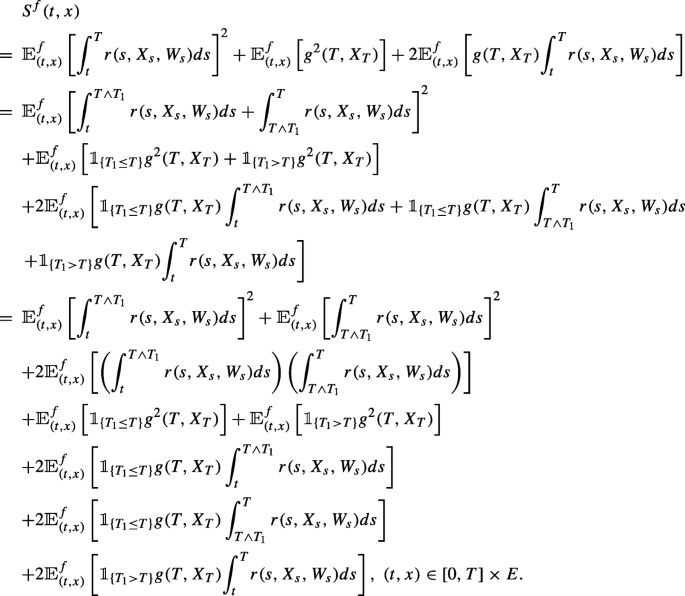
For simplicity of notation, let

We next compute L₁, L₂,…, and L₈. First, since X_s = Z₀ = x for all s < T₁, we obtain

Second, using the properties (2.3) and (2.4) yields

Third, it follows from the properties (2.3) and (2.4) again that

Thus, for every (t, x) ∈ [0, T] × E, we have

$$\begin{array}{@{}rcl@{}} && S^{f}(t,x) \\&=& {{\int}_{t}^{T}} q(z,x,f(z,x)) e^{-{{\int}_{t}^{z}} q(v,x,f(v,x))dv} \left[{{\int}_{t}^{z}} r(s, x,f(s,x))ds \right]^{2} dz\\ && + e^{-{{\int}_{t}^{T}} q(v,x,f(v,x))dv} \left[{{\int}_{t}^{T}} r(s, x, f(s,x))ds +g(T,x)\right]^{2} \\ && + {{\int}_{t}^{T}} {\int}_{E\setminus\{x\}} q(dy| z,x,f(z,x)) e^{-{{\int}_{t}^{z}} q(v,x,f(v,x))dv} \left[ 2 V^{f}(z,y){{\int}_{t}^{z}} r(s, x,f(s,x))d s + S^{f}(z,y) \right]dz. \end{array} $$

Multiplying by $e^{-{{\int }_{0}^{t}} q(v,x,f(v,x))dv}$ both sides of the above equality yields

$$\begin{array}{@{}rcl@{}} && S^{f}(t,x) e^{-{{\int}_{0}^{t}} q(v,x,f(v,x))dv} \\ &=& {{\int}_{t}^{T}} q(z,x,f(z,x)) e^{-{{\int}_{0}^{z}} q(v,x,f(v,x))dv} \left[{{\int}_{t}^{z}} r(s, x,f(s,x))ds \right]^{2} dz\\ && + e^{-{{\int}_{0}^{T}} q(v,x,f(v,x))dv} \left[{{\int}_{t}^{T}} r(s, x, f(s,x))ds +g(T,x)\right]^{2} \\ && + {{\int}_{t}^{T}} {\int}_{E\setminus\{x\}} q(dy| z,x,f(z,x)) e^{-{{\int}_{0}^{z}} q(v,x,f(v,x))dv}\left[2 V^{f}(z,y) {{\int}_{t}^{z}} r(s, x,f(s,x))ds + S^{f}(z,y) \right]dz. \end{array} $$

Differentiating both sides of the above equality with respect to t, we have

$$\begin{array}{@{}rcl@{}} && {S^{f}_{t}}(t,x) e^{-{{\int}_{0}^{t}} q(v,x,f(v,x))dv}+ S^{f}(t,x) e^{-{{\int}_{0}^{t}} q(v,x,f(v,x))dv} (- q(t,x,f(t,x))) \\ &=& -2 r(t,x, f(t,x)) {{\int}_{t}^{T}} q(z,x,f(z,x)) e^{-{{\int}_{0}^{z}} q(v,x,f(v,x))dv} \left[{{\int}_{t}^{z}} r(s, x,f(s,x))ds \right] dz\\ && -2 r(t,x, f(t,x)) e^{-{{\int}_{0}^{T}} q(v,x,f(v,x))dv} \left[{{\int}_{t}^{T}} r(s, x, f(s,x))ds + g(T,x)\right] \\ && -2 r(t,x, f(t,x)) {{\int}_{t}^{T}} {\int}_{E\setminus\{x\}} q(dy| z,x,f(z,x)) e^{-{{\int}_{0}^{z}} q(v,x,f(v,x))dv} V^{f}(z,y) dz\\ && - {\int}_{E\setminus\{x\}} q(dy| t,x,f(t,x)) e^{-{{\int}_{0}^{t}} q(v,x,f(v,x))dv} S^{f}(t,y) \ \ \forall (t,x) \in [0,T] \times E. \end{array} $$

Dividing by $e^{-{{\int }_{0}^{t}} q(v,x,f(v,x))dv}$ both sides of the above equality and using Lemma 3.2 yield

$$\begin{array}{@{}rcl@{}}&& {S^{f}_{t}}(t,x) - q(t,x,f(t,x)) S^{f}(t,x) \\ &=& -2 r(t,x, f(t,x)) \left[ {{\int}_{t}^{T}} q(z,x,f(z,x)) e^{-{{\int}_{t}^{z}} q(v,x,f(v,x))dv} \left( {{\int}_{t}^{z}} r(s, x,f(s,x))ds \right) dz\right.\\ && + e^{-{{\int}_{t}^{T}} q(v,x,f(v,x))dv} \left( {{\int}_{t}^{T}} r(s, x, f(s,x))ds +g(T,x)\right)+ {{\int}_{t}^{T}} {\int}_{E\setminus\{x\}} q(dy| z,x,f(z,x)) \\ && \left.\cdot e^{-{{\int}_{t}^{z}} q(v,x,f(v,x))dv} V^{f}(z,y) dz \right]- {\int}_{E\setminus\{x\}} q(dy| t,x,f(t,x)) S^{f}(t,y) \\ &=& -2 r(t,x, f(t,x)) \left[ e^{-{{\int}_{t}^{T}} q(v,x,f(v,x))dv}g(T,x) + {{\int}_{t}^{T}} e^{-{{\int}_{t}^{z}} q(v,x,f(v,x))dv} \left( r(z, x,f(z,x)) \right.\right.\\ && + \left.\left. {\int}_{E\setminus\{x\}} q(dy| z,x,f(z,x)) V^{f}(z,y)\right) dz \right] - {\int}_{E\setminus\{x\}} q(dy| t,x,f(t,x)) S^{f}(t,y) \\ &=& -2 r(t,x, f(t,x)) V^{f}(t,x) - {\int}_{E\setminus\{x\}} q(dy| t,x,f(t,x)) S^{f}(t,y) \ \ \forall (t,x) \in [0,T) \times E. \end{array} $$

Hence, we obtain the formula

$$\begin{array}{@{}rcl@{}} \left\{ \begin{array}{lll} {S^{f}_{t}}(t,x) + 2 r(t,x, f(t,x)) V^{f}(t,x) + {\int}_{E} q(dy| t,x,f(t,x)) S^{f}(t,y)= 0, \\ S^{f}(T,x)=g^{2}(T,x), \end{array} \right. \ \ (t,x) \in [0,T) \times E. \end{array} $$

Clearly, for every $f \in \mathbb {F}_{h}$, S^f satisfies the differential equation

$$\begin{array}{@{}rcl@{}} \left\{ \begin{array}{lll} {S^{f}_{t}}(t,x) + 2 r(t,x, f(t,x)) h(t,x) + {\int}_{E} q(dy| t,x,f(t,x)) S^{f}(t,y)= 0, \\ S^{f}(T,x)=g^{2}(T,x), \end{array} \right. (t,x) \in [0,T) \times E. \end{array} $$

On the other hand, it is easy to verify that S^f is in $\mathbb {C}_{w^{2}, \hat {w}}^{0,1}([0,T] \times E)$ under Assumptions 2.1, 3.1, 4.1 and 4.2.

Finally, note that C_h(t, x, a) := 2r(t, x, a)h(t, x) is w²-bounded under Assumptions 2.1 and 3.1. With w and $\bar {w}$ in lieu of w² and $\hat {w}$ in Theorem 3.2, respectively, it follows from Assumptions 4.1 and 4.2 that

$$\begin{array}{@{}rcl@{}} \hat{V}^{f}(t,x):=\mathbb{E}^{f}_{(t,x)} \left[ {{\int}^{T}_{t}} C_{h}(s, X_{s}, W_{s})d s +g^{2}(T,X_{T}) \right], (t,x) \in [0,T] \times E, \end{array} $$

is the unique solution in $\mathbb {C}_{w^{2}, \hat {w}}^{0,1}([0,T] \times E)$ to the equation

$$\begin{array}{@{}rcl@{}} \left\{ \begin{array}{lll} u_{t}(t,x) + 2 r(t,x, f(t,x)) h(t,x) + {\int}_{E} q(dy| t,x, f(t,x)) u(t,y)= 0, \\ u(T,x)=g^{2}(T,x), \end{array} \right. (t,x) \in [0,T) \times E. \end{array} $$

Hence, we must have $S^{f}(t,x)= \mathbb {E}_{(t,x)}^{f} \left [{{\int }_{t}^{T}} C_{h}(s,X_{s}, f(s,X_{s})ds +g^{2}(T,X_{T}) \right ]$, for every (t, x) ∈ [0, T] × E and $f \in \mathbb {F}_{h}$. □

Proof of Lemma 4.2

• (a) Using a similar argument to the proof of Lemma 8.3.7 in Hernández-Lerma and Lasserre (1999), part (a) follows from Assumption 3.3(c) and Assumption 4.3.

• (b) Fix (t, x) ∈ [0, T] × E. To show A_h(t, x) is compact, it suffices to prove A_h(t, x) is closed because A_h(t, x) ⊂ A(t, x) and A(t, x) is compact. Indeed, let {a_n}⊂ A_h(t, x) such that a_n → a ∈ A(t, x). Then, for each n, we have

  $$\begin{array}{@{}rcl@{}} h_{t}(t,x)+r(t,x,a_{n})+ {\int}_{E} h(t,y)q(dy|t,x,a_{n}) = 0. \end{array} $$

  Since $h \in \mathbb {B}_{w}([0,T] \times E)$ under Assumptions 2.1 and 3.1, by Assumption 3.3, ${\int }_{E} h(t,y) q(dy|t,x,a)$ is continuous in a ∈ A(t, x). Thus, let n →∞ in the above equality, we obtain

  $$\begin{array}{@{}rcl@{}} h_{t}(t,x)+r(t,x,a)+ {\int}_{E} h(t,y)q(dy|t,x,a) = 0, \end{array} $$

  which implies that a ∈ A_h(t, x).

□

Proof of Theorem 4.3

We prove (a) and (b) together. First, note that under Assumptions 2.1, 3.1 and 3.2, Theorem 3.2(b) implies that a policy $f \in \mathbb {F}$ is in $\mathbb {F}_{h}$ if and only if f(t, x) ∈ A_h(t, x) for all (t, x) ∈ [0, T) × E. Now, by Theorem 4.2, we know that v^∗ verifies the HJB equation

$$\begin{array}{@{}rcl@{}} \left\{ \begin{array}{lll} v^{*}_{t}(t,x)+\inf_{a\in A_{h}(t,x)}\left[2 r(t,x,a) h(t,x) + {\int}_{E}v^{*}(t,y)q(dy|t,x,a) \right] = 0, \\ v^{*}(T,x)=g^{2}(T,x), \end{array} \right. (t,x) \in [0,T) \times E. \end{array} $$

Hence, for all $f \in \mathbb {F}_{h}$ and (t, x) ∈ [0, T) × E,

$$\begin{array}{@{}rcl@{}} v^{*}_{t}(t,x)+ 2 r(t,x,f(t,x)) h(t,x) + {\int}_{E}v^{*}(t,y)q(dy|t,x,f(t,x)) \geq 0. \end{array} $$

(A.4)

Under Assumptions 4.1 and 4.2, the Dynkin’s formula in Theorem 3.1 also holds for functions $u \in \mathbb {C}_{w^{2}, \hat {w}}^{0,1}([0,T] \times E)$. Since v^∗ is in $\mathbb {C}_{w^{2}, \hat {w}}^{0,1}([0,T] \times E)$ by Theorem 4.2, using Eq. A.4, the Dynkin’s formula and Theorem 4.1 yields that

$$\begin{array}{@{}rcl@{}} S^{f}(t,x) = \mathbb{E}_{(t,x)}^{f} \left[{{\int}_{t}^{T}} C_{h}(s,X_{s},f(s,X_{s})ds +g^{2}(T,X_{T}) \right] \geq v^{*}(t,x). \end{array} $$

Thus, S^∗(h, t, x) ≥ v^∗(t, x).

On the other hand, under Assumptions 2.1, 3.1, 3.3 and 4.3, the measurable selection theorem and Lemma 4.2 ensure the existence of $f^{*}_{h} \in \mathbb {F}_{h}$ satisfying

$$\begin{array}{@{}rcl@{}} v^{*}_{t}(t,x)+ 2 r(t,x,f^{*}_{h}(t,x)) h(t,x) + {\int}_{E}v^{*}(t,y)q(dy|t,x,f^{*}_{h}(t,x))= 0, (t,x)\in [0,T) \times E. \end{array} $$

It then follows from Theorem 4.1(b) that $v^{*}(t,x)=S^{f^{*}_{h}}(t,x)\geq S^{*}(h,t,x)$, which together with S^∗(h, t, x) ≥ v^∗(t, x) yields that

$$\begin{array}{@{}rcl@{}} S^{f^{*}_{h}}(t,x)=v^{*}(t,x)=S^{*}(h,t,x), \ (t,x) \in [0,T]\times E. \end{array} $$

Since v^∗ is in $\mathbb {C}_{w^{2}, \hat {w}}^{0,1}([0,T] \times E)$, S^∗(h) is also in $\mathbb {C}_{w^{2}, \hat {w}}^{0,1}([0,T] \times E)$. □

References

Bäuerle N, Rieder U (2011) Markov decision processes with applications finance to universitext. Springer, Heidelberg
Boucherie RJ, van Dijk NM (2017) Markov decision processes in practice. Springer, Switzerland
Ghosh MK, Saha S (2012) Continuous-time controlled jump Markov processes on the finite horizon. Optimization, control, and applications of stochastic systems. Birkhäuser, New York
Guo XP, Song XY (2009) Mean-variance criteria for finite continuous-time Markov decision processes. IEEE Trans Automat Control 54:2151–2157
Guo XP, Hernández-Lerma O (2009) Continuous-time Markov decision processes. Springer, Now York
Guo XP, Ye L, Yin G (2012a) A mean-variance optimization problem for discounted Markov decision processes. European J Oper Res 220:423–429
Guo XP, Huang YH, Song XY (2012b) Linear programming and constrained average optimality for general continuous-time Markov decision processes in history-dependent policies. Linear SIAM J Control Optim 50:23–47
Guo XP, Huang XX, Huang YH (2015a) Finite horizon optimality for continuous-time Markov decision processes with unbounded transition rates. Adv Appl Probab 47:1064–1087
Guo XP, Huang XX, Zhang Y (2015b) On the first passage g-mean-variance optimality for discounted continuous-time Markov decision processes. SIAM J Control Optim 53:1406–1424
Hernández-Lerma O, Lasserre JB (1999) Further topics on discrete-time Markov control processes. Springer, New York
Hernández-Lerma O, Vega-Amaya O, Carrasco G (1999) Sample-path optimality and variance-minimization of average cost Markov control processes Sample-path. SIAM J Control Optim 38:79–93
Huang YH, Guo XP (2015) Mean-variance problems for finite horizon semi-Markov decision processes. Appl Math Optim 72:233–259
Jacod J (1975) Multivariate point processes: predictable projection, Radon-Nikodym derivatives, representation of martingales. Z Wahrscheinlichkeitstheorie und Verw Gebiete 31:235–253
Kitaev MY (1985) Semi-Markov and jump Markov controllable models: average cost criterion. SIAM Theory Probab Appl 30:272–288
Mannor S, Tsitsiklis JN (2013) Algorithmic aspects of mean-variance optimization in Markov decision processes. European J Oper Res 231:645–653
Mendoza-Pérez AF, Hernández-Lerma O (2012) Variance-minimization of Markov control processes with pathwise constraints. Optimization 61:1427–1447
Miller BL (1968) Finite state continuous time Markov decision processes with a finite planning horizon. SIAM J Control 6:266–280
Piunovskiy A, Zhang Y (2011) Discounted continuous-time Markov decision processes with unbounded rates: the convex analytic approach. SIAM J control Optim 49:2032–2061
Pliska SR (1975) Controlled jump processes. Stoch Process Appl 3:259–282
Prieto-Rumeau T, Hernández-Lerma O (2009) Variance minimization and the overtaking optimality approach to continuous-time controlled Markov chains. Math Meth Oper Res 70:527–540
Piunovskiy A, Zhang Y (2014) Discounted continuous-time Markov decision processes with unbounded rates and randomized history-dependent policies: the dynamic programming approach. 4OR-Q J Oper Res 12:49–75
Xia L (2016) Optimization of Markov decision processes under the variance criterion. Automatica 73:269–278
Yushkevich AA (1977) Controlled Markov models with countable state space and continuous time. SIAM Theory Probab Appl 22:215–235
Yushkevich AA (1980) On reducing a jump controllable Markov model to a model with discrete time. SIAM Theory Probab Appl 25:58–69
Acknowledgments
This work was supported by NSFC (No.11471341).
Author information
Authors and Affiliations
Corresponding author
Additional information
Publisher’s Note
Springer Nature remains neutral with regard to jurisdictional claims in published maps and institutional affiliations.