Unsupervised adaptation of PLDA models for broadcast diarization

Abstract

We present a novel model adaptation approach to deal with data variability for speaker diarization in a broadcast environment. Expensive human annotated data can be used to mitigate the domain mismatch by means of supervised model adaptation approaches. By contrast, we propose an unsupervised adaptation method which does not need for in-domain labeled data but only the recording that we are diarizing. We rely on an inner adaptation block which combines Agglomerative Hierarchical Clustering (AHC) and Mean-Shift (MS) clustering techniques with a Fully Bayesian Probabilistic Linear Discriminant Analysis (PLDA) to produce pseudo-speaker labels suitable for model adaptation. We propose multiple adaptation approaches based on this basic block, including unsupervised and semi-supervised. Our proposed solutions, analyzed with the Multi-Genre Broadcast 2015 (MGB) dataset, reported significant improvements (16% relative improvement) with respect to the baseline, also outperforming a supervised adaptation proposal with low resources (9% relative improvement). Furthermore, our proposed unsupervised adaptation is totally compatible with a supervised one. The joint use of both adaptation techniques (supervised and unsupervised) shows a 13% relative improvement with respect to only considering the supervised adaptation.

1 Introduction

Speaker diarization is the task intended to annotate an input audio document in terms of the speaker talking at each time. Diarization allows the indexation of audio streams and databases and supports other tasks such as speaker recognition or automatic speech recognition as well. A great effort on diarization research has been motivated by the increasing amount of available data, gathered in the wild. This type of data, too abundant to be manually tagged, becomes truly valuable if trustworthy speaker labels can be inferred. Moreover, diarization is a well-defined problem with multiple available resources, but still far from a general solution.

Some diarization overviews, such as [1, 2], provide a wide point of view of the state of the art in diarization, being the most popular approach, the bottom-up clustering strategy. This strategy consists of two steps: the segmentation of some input audio into fragments with only one active speaker and the posterior clustering of the obtained segments in terms of their speaker representations. These speaker representations have been usually constructed relying on speaker recognition models (Joint Factor Analysis or JFA [3], i-vectors [4], and Probabilistic Linear Discriminant Analysis or PLDA [5], etc.) and combined according to different clustering metrics and strategies: from Agglomerative Hierarchical Clustering (AHC) using Bayesian Information Criterion (BIC) [6] to K-means on eigenvoices [7] or PLDA Variational Bayes (VB) [8, 9].

Diarization must take advantage of the inter-speaker variability while compensating the intra-speaker variability, its main source of degradation. When considering broadcast audio, the intra-speaker variability depends on the show and genre. Unfortunately, there are too many particular effects from these multiple shows and genres to be properly compensated during model training. Hence, the uncompensated variability, specific for each show and genre, can cause an important loss of performance, also known as domain mismatch.

To reduce domain mismatch, modern diarization systems require in-domain data to train and adapt their models. Nevertheless, when these in-domain data are scarce, domain mismatch can only be handled by unsupervised adaptation techniques. This concept is analyzed in [10, 11], where models are successfully adapted using unlabeled in-domain data.

Compared to [11], we present a deeper study on the use of unsupervised model adaptation for speaker clustering in broadcast diarization. Our aim is to propose an effective and efficient solution for practical situations. Traditional supervised approaches require human annotated data which are very expensive to obtain. Nevertheless, we propose here to replace expensive hand-transcribed data by automatically obtained pseudo-speaker labels. For this purpose, we analyze multiple strategies and compare their performance with the traditional supervised approach. Moreover, we also propose hybrid solutions combining supervised and unsupervised techniques for situations in which a few labeled data are available.

In Section 2, we analyze the state of the art in diarization, making emphasis in the broadcast domain. Section 3 is dedicated to an analysis of variability conditions in broadcast data. The diarization reference system is described in Section 4. In Section 5, we explain in detail the concept of unsupervised adaptation, as well as the different strategies to best exploit it. Our experiments are detailed in Section 6. Finally the conclusions are expressed in Section 7.

2 Speaker diarization state of the art

Diarization is the activity of tagging some input audio in such a way that the speech of the different speakers is differentiated. This tagging problem can be understood as the search of the best speaker labels to explain some given audio.

The automatic estimation of these speaker labels has motivated a great interest in diarization towards broadcast data, with multiple contributions in the literature [12–14]. The most popular diarization philosophy is the bottom-up strategy. This approach starts with a large number of acoustic segments, each one ideally containing speech from a single speaker. The final labels are obtained by clustering these segments in terms of their active speaker.

First, an initial segmentation creates homogeneous acoustic fragments with a single active speaker. This acoustic segmentation is also known as Speaker Change Point Detection (SCPD). Considered solutions to the segmentation problem are based on metrics (e.g., BIC [15], ΔBIC [6], Generalized Likelihood Ratio [16], the Kullback-Leibler (KL) divergence [17]), statistical models such as Hidden Markov Models [18], and Deep Neural Networks (DNNs) [19].

The obtained variable-length segments are usually transformed into fixed-dimension representations. These representations are designed to take advantage of the inter-speaker variability while minimizing the within-speaker variability. Speaker recognition state-of-the-art techniques are usually considered for these representations, including Gaussian Mixture Models [20], JFA [3], i-vectors [4], and PLDA [5]. In this area, neural networks also contribute with solutions such as [21, 22].

Afterwards, the clustering stage groups the audio fragments so that those segments from the same speaker are clustered together. The optimal solution for the clustering problem is a brute force approach, comparing all possible arrangements of segments. However, the number of possible combinations significantly increases with the number of segments and clusters, making this solution unfeasible in practice [23]. Therefore, suboptimal solutions must be considered. Some approaches make clustering decisions relying on pairwise relationships between representations, such as AHC [10, 24–26]. Other approaches make use of relationships among multiple segments in a limited area, e.g., Mean-Shift (MS) [27–31]. Decisions can also be made keeping in mind all the acoustic segments, as K-means [7, 32], variational Bayes [33], and fully Bayesian PLDAs [8, 9, 34].

The speaker clustering task in diarization must deal with a set of challenges. The first one is the length of the homogeneous acoustic segments. State-of-the-art speaker recognition representations require a considerable amount of audio to be robust. However, these representations are unreliable when estimated from short segments as in diarization (10 s or less). The uncertainty about the number of speakers is another challenge. This uncertainty influences the tradeoff between cluster and speaker impurity. On the one hand, an overestimation of the speaker number divides real speakers into different clusters, though these clusters are usually purer. On the other hand, the underestimation of speakers is bound to detect the largest clusters, i.e., the most talkative speakers, including spurious audio from the least talkative speakers, who can be lost. This loss of speakers is sometimes unacceptable, specially when these less talkative speakers are the most relevant ones. In fact, the distribution of the amount of speech among speakers is an important factor to properly determine the number of speakers in a recording. The less uniform the distribution, the less data we have to properly represent certain speakers, but the lower amount of speech can be improperly modeled. Broadcast data include extreme cases reaching up to 60–70 speakers in a 1-h show, in which 2–3 speakers can be responsible for 70% of the audio. Another problem is caused by the assumption of homogeneous acoustic conditions along the whole audio. Factors such as background noise or reverberation can temporally alter the audio characteristics along a recording. For example, audio broadcast is recorded in multiple locations such as studio, streets, and sports events. Besides, broadcasted audio sometimes includes background sounds, such as music, applauses, and laughs, deliberately added loud enough to emphasize certain show conditions.

3 Analysis of the broadcast audio scenario

Broadcast environment is widely known due to the large diversity of shows and genres. Each scenario has its own characteristics, completely different from each other, including multiple recording locations, or postprocessing additions, generating a great variability. In fact, there is also within-show variability, because of the different parts of the show. An example can be the news, with studio conditions and outdoor reports.

The Multi-Genre Broadcast (MGB) Challenge 2015 [14] dataset is a suitable choice to analyze variability in broadcast data. The dataset includes about 1600 h of audio taken from the British Broadcasting Corporation, coming from about 500 different shows and divided into three subsets: train, development, and test. This large amount of data makes this dataset a good choice to study how different factors impact performance because of the wide range of shows and genres. Two important factors are the variability in the number of speakers and the distribution of the amount of speech among speakers. The larger the uncertainty in the number of speakers, the larger is the possible error in its estimation and its impact in the performance. This variability is influenced by the distribution of the amount of speech among speakers. The more available audio from one speaker, the easier to identify him or her. Therefore, quiet speakers are poorly represented and can be easily lost.

We present Fig. 1 to show the variability in the speaker count for each show in development and evaluation subsets. The involved shows in the development subset are “Doctor Who” (DW), “UEFA Euro 2008 Match” (UE08M), “The Alan Clark Diaries” (TACD), “Springwatch” (SW), and “Last of the Summer” (LOTS). The evaluation set consists of episodes from “Celebrity Masterchef” (CM) and “The Culture Show Uncut” (TCSU). Each column analyzes a single show, illustrating the spread of the number of speakers along its episodes. As we can see, the number of speakers presents significant differences among the different shows (up to 30 speakers between median values of shows UE08M and TCSU) and within the shows, with deviations up to 20 speakers between episodes of the same show (CM and TCSU).

Fig. 1

Number of speakers per show. Shows DW, UE08M, TACD, SW, and LOTS correspond to development set. CM and TCSU shows belong to evaluation set

In Fig. 2, we illustrate the ratio of speech for the most talkative speaker in each episode from both development and evaluation subsets. Again, a large uncertainty is shown, having differences between shows up to 60% (shows TACD and LOTS) and presenting deviations of 10% from the median. Besides, no correlation can be observed between the variability caused by the number of speakers and the speech distribution variability.

Fig. 2

Proportion of speech for the most active speaker per show. Shows DW, UE08M, TACD, SW, and LOTS correspond to development set. CM and TCSU shows belong to evaluation set

This analysis can be expanded by moving to single episodes. In Fig. 3, we illustrate the ratio of speech activity per speaker for two episodes with a very different speaker distribution. While Fig. 3a depicts an episode with a dominant speaker (almost 70% of the speech), Fig. 3b reflects a more even speech distribution, in which no speaker exceeds a 20% of total speech and 10 speakers make significant contributions (more than 5% of speech).

Fig. 3

Distribution of speech per speaker for two episodes: a An episode with a dominant speaker. b An episode with a more even speech distribution

4 Baseline diarization system

The reference diarization system [34] makes use of the standard bottom-up strategy, first dividing the input audio into segments with only one active speaker and clustering them according to the i-vector [4] PLDA [5] framework. Its schematic block diagram can be seen in Fig. 4.

Fig. 4

Reference diarization system schematic

First the system converts the input audio into a stream of Mel Frequency Cepstral Coefficients (MFCCs). Simultaneusly, Voice Activity Detection (VAD) is carried out. In our system, the VAD mask is inferred by means of a DNN. This network analyzes the input features along a short-duration sliding window, moved along the stream of MFCC frames. In each window, the DNN estimates a VAD label per input MFCC feature vector. The considered DNN makes use of Bidirectional Long Short Time Memory (BLSTM) [35] layers, a type of Recurrent Neural Networks which analyze the MFCC stream as a sequence. These BLSTM layers consists of two Long Short Time Memory [36] layers, which analyze the same input sequence but in opposite directions.

Given the features and the VAD mask, we perform a BIC-based [6] segmentation. BIC [15] is a model selection criterion, i.e., a method to choose the model which better describes some given data X. BIC is a likelihood criterion penalized by the model complexity, the number of parameters in the model. For SCPD, we use ΔBIC [6] to determine the model that best describes some given data X. In hypothesis H₀, we model the data with a single Gaussian distribution, as if it comes from a single speaker. H₁ assumes that data X contains frames from two speakers, separated by a single speaker boundary. Each speaker is then modeled by its own Gaussian distribution. In our experiments, these Gaussian distributions for both H₀ and H₁ have full-rank covariance matrix. The formulation for ΔBIC is:

$$ \Delta\text{BIC}(\mathrm{X},{\lambda})=\log(P({\mathrm{X}|H_{1}}))-\log(\mathrm{P}{X|H_{0}})-{\lambda} R $$

(1)

where R represents the penalty term to compensate the excess of parameters in H₁ models with respect to H₀, and λ is a finetuning parameter. The described comparison is repeated along the feature stream using a sliding window, considering multiple samples per analysis window as candidate boundaries.

For each obtained segment, we compute an i-vector. I-vectors are centered, whitened, and length-normalized [37] (normalized so its Euclidean norm is equal to 1), obtaining the set of N i-vectors Φ_n={ϕ_n1,..,ϕ_nN} for episode n.

These i-vectors are then clustered to obtain the final partition Θ_n={θ_n1,..,θ_nN}. The i-vector clustering is performed in terms of a PLDA model. Figure 5 illustrates the clustering step. An initial clustering is constructed with AHC based on PLDA pairwise log-likelihood ratio. A posterior resegmentation is performed by means of a fully Bayesian PLDA with soft speaker labels [9], which redistributes the segments along the clusters given by the initialization. In order to mitigate the initialization influence, multiple evaluations are simultaneously performed. K different initial partitions ${\Theta '}_{n}^{k}$ are obtained by means of the agglomerative clustering. These initializations come from different levels in the AHC dendrogram, containing a different number of speakers. Each initialization ${\Theta '}_{n}^{k}$ is resegmented obtaining the diarization labels $\Theta _{n}^{k}$. The final diarization labels Θ_diar are chosen by maximizing the variational Evidence Lower Bound (ELBO) [38], which measures how well the model fits the given data. Although the prior over Θ should penalize models with more complexity (more speakers), we empirically observed that the ELBO criterion overestimates the number of speakers. Consequently, a modified ELBO with a penalty term to compensate different model complexities [39] is considered instead.

Fig. 5

Clustering step. Given some set of i-vectors Φ_n and a PLDA model $\mathcal {M}_{\text {diar}}$, diarization labels Θ_diar are obtained

4.1 Fully Bayesian PLDA

PLDA is a statistical generative model proposed in [5]. This model represents a population of N i-vectors ϕ_j generated by M speakers, with N_i i-vectors from the speaker i. Each i-vector ϕ_j produced by the speaker i is modeled as

$$ \phi_{j}=\mu + \mathbf{Vy}_{i} + \boldsymbol{\epsilon}_{j} $$

(2)

where μ represents the overall mean of the training dataset. y_i is a speaker dependent latent variable, an eigenvoice. All i-vectors from the same speaker share the same value for this variable, and its expected value given an audio can be used to represent the identity of an individual. This variable is assumed to follow a standard normal distribution. V is the matrix describing the inter-speaker variability subspace of dimension D. Finally, ε_j is the intra-speaker variability term, unique for each i-vector j, and modeled as a zero-mean normal distribution with W⁻¹ full-rank covariance matrix. The Gaussian assumption about the priors makes the conditional probability of the i-vector ϕ_j with respect to the latent variables to follow a Gaussian distribution as:

$$ P({\phi_{j}|\mathbf{y}_{i}})=\mathcal{N}\left({\phi_{j}}|{\mu+\mathbf{V}\mathbf{y}_{i},}{\mathbf{W}^{-1}}\right) $$

(3)

The corresponding Bayesian network for this model is illustrated in Fig. 6a.

Fig. 6

Bayesian network of the employed PLDAs. a Simplified PLDA. b Fully Bayesian PLDA

A Bayesian PLDA is proposed in [8, 9], upgrading the model by formulating the fully Bayesian PLDA with speaker labels modeled by latent variables. This model substitutes the fixed speaker assignment by a set of discrete latent variables Θ={θ₁,θ₂,..,θ_N}. This modification assumes that a set of N i-vectors Φ={ϕ₁,ϕ₂,..,ϕ_N} is produced by M speakers, so that each i-vector comes from an unknown speaker i=1,...,M. All the speakers are modeled by an eigenvoice y_i, conforming the set $\mathbf {Y}=\{\mathbf {y}_{1},..,\mathbf {y}_{M}\}\in \mathbb {R}^{D}$. The assignment of i-vectors to the speakers is controlled by the new latent variable θ_ij. For this purpose θ_ij takes the value of one if the i-vector ϕ_j belongs to the speaker i and zero otherwise. The definition of the likelihood for an i-vector ϕ_j is:

$$ P{(\phi_{j}|\mathbf{Y},\theta_{j})}= \prod_{i=1}^{M}\mathcal{N}(\phi_{j}| \mu + \mathbf{V}\mathbf{y}_{i},\mathbf{W}^{-1}){}^{\theta_{ji}} $$

(4)

where latent variable Θ follows a multinomial distribution. This distribution has a prior on its parameter π_θ, which a priori determines the expected probability of assignment to each cluster. This prior distribution π_θ follows a Dirichlet distribution.

Furthermore, the model parameters (μ, V, W) are substituted by latent variables too. We opt for a Gaussian prior for the mean μ. The matrix V is defined in terms of its columns, each one with a Gaussian prior. Finally, we place a Wishart prior for the matrix W. A more detailed explanation of the model parameter priors is available in [9]. Figure 6b depicts the Bayesian network of this PLDA model.

The complexity of the proposed model makes its training and evaluation not straightforward. Instead, a VB decomposition is proposed approximating the joint posterior distribution P(Z|Φ) by a factorial distribution q(Z), where Z represents the whole set of latent variables in the original model (Y,Θ,π_θ,μ, V and W). For simplicity, q(Z) is formulated as a product of distributions, also known as factors. Each factor is the approximate posterior of a limited subset of latent variables with respect to the given data. The posterior of our proposed PLDA model is factorized as:

$$\begin{array}{*{20}l} &P({\mathbf{Y},\Theta,\boldsymbol{\pi}_{\theta},\mu,\mathbf{V},\mathbf{W},\alpha|\Phi})\\ \approx&q({\mathbf{Y}})q({\Theta})q({\boldsymbol{\pi}_{\theta}})q({\mu,\mathbf{V}})q({\mathbf{W}})q({\alpha}) \end{array} $$

(5)

In this situation, the log-likelihood of the original model consists of the sum of two terms,

$$ \ln P({\Phi})=\mathcal{L}\left(q({\mathbf{Z}}) \right) + \text{KL}\left(q(\mathbf{Z}) ||P({\mathbf{Z}|\Phi})\right) $$

(6)

the Variational Lower Bound, also known as ELBO, and the KL divergence of the true posterior with respect to its approximation. Both the training of this model and the evaluation are carried out by the iterative reevaluation of the described factors, maximizing the ELBO. While training needs the reevaluation of all the factors, during evaluation only those factors related to the speaker labels q(Θ) (q(Y),q(Θ) and q(π_θ)) are required to be iteratively updated.

This variational Bayes method provides a useful tool for diarization. We can assume that the best diarization labels Θ_diar are those which best explain the given i-vectors Φ, measured by the ELBO. By reevaluating the factor q(Θ) (and the related q(Y)q(π_θ)) we can maximize the ELBO term. A collateral effect of this VB solution is that it performs its own estimation of the number of speakers. The VB decomposition distributes i-vectors among the different hypothetical clusters. In the meanwhile, the VB solution can consider a cluster not responsible for any contribution, deciding that the given data is well explained using fewer clusters. These empty clusters are discarded.

The variational Bayes decomposition allows a closed-form solution for a simplified version of the original model. Unfortunately, it also creates a strong dependence on the initialization values for the latent variables, especially the clustering ones. We include a solution to mitigate this drawback, deterministic annealing [40]. This technique smooths the ELBO function. This concept assumes the real and smoothed ELBO should have close global maxima. Under this assumption, latent variables converge according to a simpler version of the ELBO function, being fine-tuned afterwards as the smoothing gets relaxed.

5 Methods for domain mismatch reduction

PLDA performance is known to suffer from strong degradation when facing a domain mismatch between training and evaluation conditions. The same kind of mismatch we previously observed in broadcast data when studying the differences among episodes, shows, and genres. The large number of different domains makes training particular models unfeasible, so domain adaptation is the best option.

Adaptation in models with speaker awareness (e.g., PLDA) requires some speaker labels Θ_ADAPT, as illustrated in Fig. 7a. This is also referred as supervised adaptation. However, in many situations, perfect labeled in-domain data is either limited or just unavailable. For those situations, in [11], it was proposed the unsupervised adaptation with pseudo-speaker labels (Fig. 7b). The necessary speaker labels Θ_ADAPT were estimated only considering the evaluation data.

Fig. 7

Schematic for the a supervised and b unsupervised adaptation. $\mathcal {M}_{\text {REF}}$ represents the source model and $\mathcal {M}_{\text {ADAPT}}$ the adapted model. Φ_ADAPT and Θ_ADAPT are the i-vectors and labels to adapt, respectively

In [11], it was presented our basic unsupervised adaptation block, based on the adaptation approach proposed in [9]. Given a PLDA model trained with out-of-domain data, we want its parameters tuned to explain another domain making use of some unlabeled data. Due to the fact that our model follows a Bayesian approach, we must obtain the tuned distributions for the parameters μ, V and W, as well as for their priors (α). Because we use unlabeled data, some inferred labels must be used. These labels are not totally reliable, so our adaptation approach must also take into account some out-of-domain data as well. A maximum likelihood solution for our adaptation approach is not analytically tractable; thus, we make use of an approximation by means of VB. According to this approximation, the joint posterior distribution is factorized as follows:

$$\begin{array}{*{20}l} P({\mathbf{Y},\mathbf{Y}_{d},\Theta, \pi_{\theta},\mu,\mathbf{V},\mathbf{W},\alpha | \Phi,\Phi_{d}}) \approx \\ q({\mathbf{Y},\mathbf{Y}_{d}})q({\Theta})q({\pi_{\theta}})q({\mu,\mathbf{V}})q({\mathbf{W}})q({\alpha}) \end{array} $$

(7)

where Φ represents the in-domain i-vectors. These i-vectors are explained by the latent variable Θ, which plays the role of the adaptation labels Θ_ADAPT. The latent variable Θ is explained in terms of its prior π_θ. Y is the speaker-dependent latent variable for the in-domain i-vectors. Φ_d symbolizes the out-of-domain i-vectors, explained with perfect labels. Y_d is the speaker latent variable to explain these i-vectors. Moreover, the model parameters (μ,V and W) are also latent variables, some of them with its own prior latent variable (α).

The adaptation is done by maximizing the ELBO term of the whole solution. Although factors q can follow any distribution, the maximization of the lower bound forces optimal factor distributions q^∗, which have a closed form formulation [38]. This formulation imposes that factors are distributions whose parameters depend on the remaining factorized distributions, forcing them to be tied. Therefore, the final model is obtained by the iterative update of the factors.

The adaptation process starts with some initial values for the speaker label latent variable Θ. The optimal factor q^∗(Y,Y_d)k for the speaker latent variables Y and Y_d is then estimated as:

$$\begin{array}{*{20}l} &\ln q^{*}({\mathbf{Y},\mathbf{Y}_{d}})= \\ &\mathrm{E}[\ln P({\Phi,\Phi_{d},\mathbf{Y},\mathbf{Y}_{d},\Theta,\pi_{\theta},\mu,\mathbf{V},\mathbf{W},\alpha})]{} \end{array} $$

(8)

taking the expectations with respect to all the latent variables except for Y and Y_d.

Once we have updated the speaker dependent factor, we now start updating those related with the parameters. First we update the optimal factor q^∗μ,V

$$\begin{array}{*{20}l} &\ln q^{*}({\mu,\mathbf{V}})= \\ &\mathrm{E}[\ln P({\Phi,\Phi_{d},\mathbf{Y},\mathbf{Y}_{d},\Theta,\pi_{\theta},\mu,\mathbf{V},\mathbf{W},\alpha})]{} \end{array} $$

(9)

whose expectation involves all latent variables with the exception of μ and V. Then, we update the optimal factor for the variable W

$$\begin{array}{*{20}l} &\ln q^{*}({\mathbf{W}})= \\ &\mathrm{E}[\ln P({\Phi,\Phi_{d},\mathbf{Y},\mathbf{Y}_{d},\Theta,\pi_{\theta},\mu,\mathbf{V},\mathbf{W},\alpha})]{} \end{array} $$

(10)

calculating the expectation with respect to all the latent variables except for W.

Because we are in a Bayesian solution, we similarly update those factors related with priors (q^∗α and q^∗π_θ), estimating the expectations with respect to all the variables except for the factor variable.

Finally, the last factor to be updated is the speaker label optimal factor q^∗Θ, calculated as:

$$\begin{array}{*{20}l} &\ln q^{*}({\Theta})= \\ &\mathrm{E}[\ln P({\Phi,\Phi_{d},\mathbf{Y},\mathbf{Y}_{d},\Theta,\pi_{\theta},\mu,\mathbf{V},\mathbf{W},\alpha})]{} \end{array} $$

(11)

where we again make the expectation for all variables except Θ. This factor is responsible for the newer version of the speaker labels, necessary to keep iterating the optimization process.

The initial values for the speaker labels Θ have a significant impact on the performance. In [11], we proposed a method to obtain these initial labels from the same audio to diarize by means of naïve clustering techniques. This work was an exploratory work about how to unsupervisedly extract speaker information for its posterior use in adaptation.

In this work, we study multiple adaptation approaches based on this unsupervised adaptation block. This adaptation is conditioned by two elements: the initial labels for the adaptation and the source model to adapt. With respect to the initial labels, our proposed approaches study the impact of speaker awareness in the pseudo-speaker label estimation. Two main options, cosine similarity, which lacks of any knowledge about the speaker subspace, and PLDA likelihood ratio are tested. Efficient clustering techniques are considered, such as AHC and MS [28–31].

Regarding the source model, we study its influence during the adaptation step depending on whether it is aware of the evaluation domain or not. In the scenario where the source model has partial knowledge about the evaluation domain, we also analyze the impact of how this awareness is obtained. On the one hand, we can consider just unlabeled data for a previous adaptation. On the other hand, this previous adaptation can also count with scarce human labeled information.

All these approaches are validated by direct comparison with the traditional supervised adaptation, performed with the same limited data. The proposed modalities are very oriented to broadcast scenarios, where the tradeoff between expenses and labeled resources is an important factor in decision making. The proposed alternatives are as follows:

• Independent unsupervised strategy

  Our first proposal is the independent unsupervised adaptation strategy, which individually performs the adaptation, episode by episode. A conceptual representation is illustrated in Fig. 8. For each episode n, we adapt the out-of-domain PLDA model $\mathcal {M}_{\text {OOD}}$ only taking into account the i-vectors Φ_n from episode n. The result is the adapted model $\mathcal {M}_{n}$.

  Fig. 8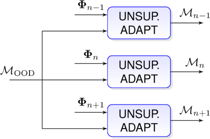

  

  Schematic for unsupervised independent adaptation for the episodes n−1, n, and n+1. $\mathcal {M}_{\text {OOD}}$ represents the out-of-domain model and $\mathcal {M}_{n-1}, \mathcal {M}_{n}$, and $\mathcal {M}_{n+1}$, and the adapted models for each episode. Φ_n−1,Φ_n and Φ_n+1 are the i-vectors from each episode

• Longitudinal unsupervised strategy

  Broadcast content from a show usually involves multiple episodes (i.e., a season). These multiple episodes are a priori likely to have similar acoustic information (same speakers and similar acoustic conditions). Therefore, we can take into account more than one episode to perform the PLDA adaptation, supervised or not. In the longitudinal approach, episode n is adapted considering the result of the adaptation $\mathcal {M}_{n-1}$ from the previous episode n−1 as a reference model. This strategy is illustrated in Fig. 9. By this way, we expect that successive adaptations could retain show-dependent information to improve the performance.

  Fig. 9

  

  Schematic for unsupervised longitudinal adaptation for the episodes n−1, n, and $n+1.\mathcal {M}_{\mathrm {n-2}}, \mathcal {M}_{n-1}, \mathcal {M}_{n}$, and $\mathcal {M}_{n+1}$ represent the adapted models for episodes n−2,n−1, n, and n+1. Φ_n−1,Φ_n, and Φ_n+1 are the i-vectors from each episode

• Independent semi-supervised strategy

  We also propose semi-supervised architectures, assuming that a few labeled data are available. In real applications, a perfectly labeled small subset of data may be available. Therefore, we want to test whether we can combine the knowledge acquired from a small subset of supervised data (e.g., one or two episodes) with the one obtained by the unsupervised adaptation.

  Our first hybrid proposal considers a model adaptation stage in terms of the supervised labeled data followed by an unsupervised domain adaptation, independent for each episode. In this approach, the out-of-domain model $\mathcal {M}_{\text {OOD}}$ is first adapted with the in-domain perfectly labeled data, obtaining the in-domain model $\mathcal {M}_{\text {ID}}$. This model is later specifically adapted to each episode using the unsupervised adaptation block. The architecture is shown in Fig. 10.

  Fig. 10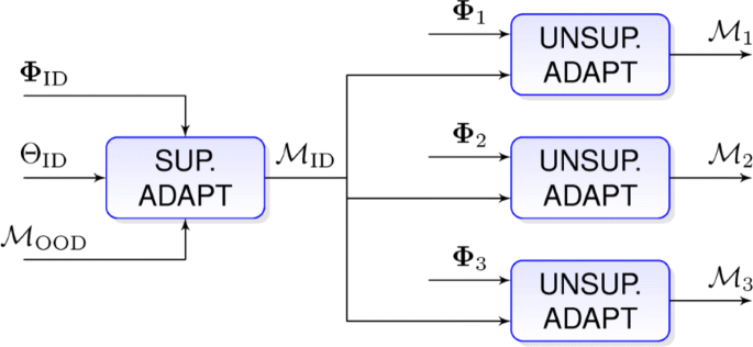

  

  Semi-supervised adaptation strategy based on the unsupervised independent adaptation approach for the episodes 1, 2, and 3. $\mathcal {M}_{\text {OOD}}$ represents the out-of-domain model, $\mathcal {M}_{\text {ID}}$ depicts the show in-domain model, and $\mathcal {M}_{1}, \mathcal {M}_{2}$, and $\mathcal {M}_{3}$ the adapted models for each episode. Φ_ID and Θ_ID symbolize the in-domain i-vectors and its speaker labels. Φ₁,Φ₂, and Φ₃ are the i-vectors from each episode

• Longitudinal semi-supervised strategy

  We also test a semi-supervised longitudinal strategy when dealing with multiple episodes from the same show. The out-of-domain model $\mathcal {M}_{\text {OOD}}$ is supervisedly adapted with the limited labeled data (i-vectors Φ_ID and labels Θ_ID), generating an in-domain model $\mathcal {M}_{\text {ID}}$. This model is then adapted in an unsupervised longitudinal way, i.e., the resulting adapted model for episode n will work as reference model for episode n+1. Its schematic is illustrated in Fig. 11.

  Fig. 11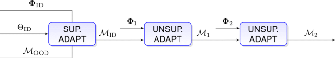

  

  Semi-supervised adaptation strategy based on the longitudinal unsupervised adaptation approach for the episodes 1 and 2. $\mathcal {M}_{\text {OOD}}$ represents the out-of-domain model, $\mathcal {M}_{\text {ID}}$ depicts the show in-domain model and $\mathcal {M}_{1}$ and $\mathcal {M}_{2}$ the adapted models for each episode. Φ_ID and Θ_ID symbolize the in-domain i-vectors and its speaker labels. Φ₁ and Φ₂ are the i-vectors from each episode

6 Results and discussion

In this section, we present our experiments and results. This analysis has been carried out considering the MGB 2015 [14]. First, we explain the performance metric DER. Then, we establish the baseline results with the system shown in Section 4. Later, we analyze the different proposed strategies based on our unsupervised adaptation, starting with the totally unsupervised strategies and studying the semi-supervised approaches afterwards.

6.1 Diarization error rate

Diarization error rate (DER) is the standard metric for the diarization task in recent times. This measure considers the ratio of the misclassified amount of audio L_ERROR with respect to the total amount of speech in the audio L_Ω.

$$ \text{DER}=\frac{L_{\text{ERROR}}}{L_{\Omega}} $$

(12)

The misclassification in the diarization process can be assigned to one of the following reasons:

• Some speech is considered non speech (miss error).

• Some non-speech is thought to contain voice (false alarm error).

• Some speech is assigned to a mistaken speaker (speaker error).

• Some period of time is not recognized to contain speech from more than one speaker (overlap error).

The sources of error are totally independent, so we can introduce them into the DER formula, and decompose the global term into different error terms to be added:

$$\begin{array}{*{20}l} \text{DER}=&\frac{L_{\text{MISS}} + L_{\mathrm{F.A.}} + L_{\text{SPK}} + L_{\text{OV}}}{L_{\Omega}} \end{array} $$

(13)

$$\begin{array}{*{20}l} =&E_{\text{MISS}} + E_{\mathrm{F.A.}} + E_{\text{SPK}} + E_{\text{OV}} \end{array} $$

(14)

where E_MISS,E_F.A.,E_SPK, and E_OV are the DER error terms for Miss Error, False Alarm Error, Speaker Error and Overlap Error respectively.

For evaluation purposes, we make use of the scoring tool released by the organization. This tool is based on the National Institute of Standards and Technology md-eval scoring tool, contained in the Speech Recognition Scoring Toolkit [41]. The configuration considers a 0.25-s collar around reference borders and excludes from the evaluation any audio with overlapped-speech.

6.2 Performance of the reference system

Our baseline system is the one described in Section 4. The diarization system considers 20-coefficient MFCCs as acoustic features, without derivatives. Short time cepstral mean and variance normalization is performed. According to these features, we use a 256-Gaussian 100-dimension i-vector extractor, trained with the train subset. A 50-dimension PLDA model is trained with the development subset, the only subset with oracle speaker labels. The results were obtained with a DNN-based VAD. This VAD consists of a 3-BLSTM-layer neural network, with 256 neurons per layer. This network is trained on the development set, inferring the VAD labels for segments of audio up to 3 s, i.e., analyzing sequences of 300 frames. Table 1 shows the results with the diarization reference system according to this configuration, analyzing the system with AHC PLDA, with and without VB resegmentation. We also include the three best results in the original MGB 2015 evaluation [14] for comparison.

Table 1 DER(%) for the reference system

Table 1 shows the poor performance of the agglomerative clustering and the significant benefits of the VB resegmentation. These results are slightly worse than those obtained by Cambridge, the winner system of the evaluation. According to its description, Cambridge system specially outperforms its competitors thanks to its VAD estimation, obtained by a DNN trained on a careful data selection from the unreliable train subset. This VAD obtains 4.3% error in the dev.full subset [43] outperforming ours, which obtains 13.1% error on the same subset. In general, the poor performance of all teams reveals the difficulty of the challenge. Moving to a more detailed analysis with our own results, not all the shows behave similarly.

Results in Table 2 present a deeper analysis of the baseline results show by show. They reveal the different behavior of the out-of-domain initial model depending on the show it is applied to, having a relevant impact on the final results (some shows are up to five times more accurate than others). While some shows are very well diarized, others obtain much poorer performances.

Table 2 DER (%) results per show with baseline system

6.3 Independent unsupervised adaptation

The previous results have shown the influence of domain mismatch when PLDA models are considered. We now evaluate the novel independent totally unsupervised adaptation strategy. We propose exploring the four possible pseudo-speaker label initializations described in [11]: two clustering modalities, AHC and MS, working with two similarity metrics, cosine similarity (COS) and PLDA log-likelihood ratio (PLDA). The results for this experiment are shown in Table 3.

Table 3 DER(%) for the unsupervised adaptation in the evaluation set

The direct comparison of Table 2 (its last line) and Table 3 show the benefits of the unsupervised adaptation. The first step in the diarization system (the agglomerative clustering with PLDA log-likelihood ratio) evidences approximate 10–20% relative improvements when adapted models are considered, regardless the pseudo-speaker labels. Besides, these results are improved by means of the variational Bayes refinement (VBPLDA resegmentation), also considering the adapted models. However, not all the pseudo-speaker labels are equally useful. Some of these labels lead to local DER minima from which the variational Bayes posterior resegmentation does not provide any extra improvement.

All the experiments with cosine similarity pseudo-speaker labels have outperformed the PLDA-based counterparts and perform better than the baseline. In fact, PLDA-based pseudo-speaker labels are harmful for adaptation purposes, getting degraded with respect to the baseline results. Moreover, in all cases MS has obtained better results than AHC.

6.4 Longitudinal unsupervised adaptation

Some of the results included in Table 3 show a significant improvement with respect to our baseline. This improvement is obtained despite considering a small amount of in-domain information (up to one hour of audio). Taking into account, multiple episodes (all the episodes from a show) with our longitudinal proposal we expect to get bigger improvements. Table 4 shows the results of the longitudinal unsupervised adaptation approach for the evaluation set. AHC and MS are studied with cosine similarity. The longitudinal adaptation is done along all the episodes from a show.

Table 4 DER(%) results for the unsupervised adaptation with longitudinal model propagation in the evaluation set

The results in Table 4 also outperform the reference, especially when MS is used. However, as in the independent adaptation, AHC behaves significantly worse than MS. For both cases, AHC and MS, the longitudinal unsupervised adaptation shows a small degradation versus the independent counterpart. This small degradation can be attributed to the consecutive adaptations with noisy data. In consequence, it is important to determine if this longitudinal strategy overcomes the independent one considering less episodes in a row. For this reason, we analyze the results episode by episode, shown in Fig. 12. We illustrate the difference between DER results obtained with the independent approach versus the longitudinal one (Δ_DER=DER_INDEP−DER_LONG) for each episodes from both shows.

Fig. 12

ΔDER (%) performance episode by episode for the two shows of the evaluation set. Defined as ΔDER=(DER_INDEP−DER_LONG). AHC refers to the agglomerative clustering pseudo-speaker labels. a Show 6: Masterchef celebrity. b Show 7: The culture show uncut

Figure 12 reveals that the longitudinal approach compared to the independent adaptation suffers from a degradation which affects similarly all the episodes. Besides, the analysis indicates this behavior is shared for both the agglomerative hierarchical pseudo-speaker labels and the MS ones. The results indicate that the degradation already appears in the second episode from both shows. Therefore, a longitudinal adaptation in few episodes is not expected to take any advantage.

6.5 Use of in-domain-labeled data and semi-supervised adaptation

In previous sections, we have reported a significant improvement of the DER measure due to the unsupervised adaptation with pseudo-speaker labels, especially with those created with MS and cosine similarity. However, we cannot compare these results with the traditional supervised adaptation because MGB dataset does not provide extra in-domain-labeled data for this purpose. Therefore, we propose an alternative dataset arrangement. We divide the evaluation set into two parts. The first one is dedicated to supervised adaptation, containing the first episode from each show to evaluate. The new evaluation subset contains all the remaining episodes from the same shows. This modification of the evaluation subset makes unfair any comparison with the previous results and those obtained in the original MGB 2015 challenge. Hence, both the baseline system and the fully unsupervised approaches must be reevaluated.

With the new distribution of data, we compare the classical supervised adaptation, with our new proposed alternatives, both the independent and the longitudinal approach. In this experiment, we have evaluated supervised adaptation with only 1-h episode for each show as in-domain information. The results are shown in Table 5.

Table 5 DER (%) results of supervised and unsupervised (independent and longitudinal) adaptation with the new data distribution in the evaluation set

The results in Table 5 show that our proposed unsupervised adaptations (independent and longitudinal approaches) outperform the supervised adaptation with the baseline system when a few in-domain data are used (1-h episode from each show). Again, the independent unsupervised adaptation approach gets the best results, obtaining up to 9% relative improvement. This result is specially noticeable because in-domain information automatically estimated from the data we are diarizing can be more informative than small amounts of manually annotated in-domain data.

The new data distribution provides perfectly labeled in-domain audio. Hence, semi-supervised approaches can also be analyzed, first applying some supervised adaptation of the models with the available labeled data and then adapt to the evaluation audio in an unsupervised fashion. In Table 6, we compare the baseline system with respect to all the proposed adaptation techniques (supervised, unsupervised independent, unsupervised longitudinal, semi-supervised independent, and semi-supervised longitudinal), evaluated with this new data distribution. Only cosine-similarity MS pseudo-speaker labels are considered.

Table 6 DER (%) results in the evaluation set with multiple adaptations of configuration: none, independent, or longitudinal unsupervised adaptation and with or without previous supervised adaptation

According to Table 6, all our totally unsupervised approaches (independent and longitudinal), obtain some boost in performance by including a supervised adaptation step, becoming semi-supervised approaches. In fact, all the results without any supervised adaptation (the baseline and the totally unsupervised adaptations) are improved similarly (approximately 2% absolute improvement). Hence supervised and unsupervised adaptations are complementary.

7 Conclusions

This paper provides a detailed analysis of domain adaptation as a solution for the problem of domain mismatch, noticeable in broadcast data. Different approaches based on supervised and specially unsupervised PLDA adaptations, including hybrid solutions, were tested. Our main goal is the validation of our novel unsupervised adaptation methods, which allow the substitution of manually obtained speaker labels by automatically obtained pseudo-speaker labels. This technology reduces the need for in-domain labeled data, with its respective reduction of expenses.

The most important result is that our novel unsupervised adaptation approaches are able to outperform a supervised adaptation when perfectly labeled in-domain data is scarce. Our results revealed up to 9% relative improvements when comparing the new totally unsupervised approaches versus a supervised adaptation. Therefore, in-domain information automatically estimated from the data we are diarizing can be more informative than small amounts of manually annotated in-domain data. Besides both adaptations, supervised and our unsupervised one, are totally compatible. The results indicate that improvements are accumulated if both adaptation approaches are applied. Our hybrid adaptations implied up to 13% relative improvement compared to considering only a supervised adaptation. All these improvements offer multiple opportunities. On the one hand, the reduction of the need for manually labeled data is possible, partially substituting hand-transcribed data with unsupervised pseudo-speaker labels. On the other hand, this technique can offer a significant boost of performance by just making a more efficient use of the available data, including the evaluation audio itself.

Despite outperforming the baseline and the supervised adaptation, not all the proposed architectures performed similarly. The results show that those strategies which deal independently with the episodes (independent adaptation) obtained better results than considering all of them (our longitudinal approach). In the context of MGB 2015, the former obtained a relative 16% improvement while the latter got a relative 13% improvement with respect to the baseline. This general loss of performance with respect to the independent adaptation approach indicates that our proposed longitudinal adaptation takes no further advantage of automatically labeled in-domain data, being degraded by the accumulated errors. Further work should find strategies that successfully make use of this available extra information.

Finally, our results reassure that simple techniques such as AHC and MS are accurate enough to generate improvements working as initialization. However, not all these labels are equally useful. All our results indicate that MS performs significantly better than the AHC, and the cosine similarity pseudo-speaker labels outperform PLDA-based ones.

References

S. E. Tranter, D. A. Reynolds, An overview of automatic speaker diarization systems. IEEE Trans. Audio Speech Lang. Process.14(5), 1557–1565 (2006). https://doi.org/10.1109/TASL.2006.878256.
X. Anguera, S. Bozonnet, N. Evans, C. Fredouille, G. Friedland, O. Vinyals, Speaker diarization: a review of recent research. IEEE Trans. Audio Speech Lang. Process.20(2), 356–370 (2012). https://doi.org/10.1109/TASL.2011.2125954.
P. Kenny, P. Ouellet, N. Dehak, V. Gupta, P. Dumouchel, A study of interspeaker variability in speaker verification. IEEE Trans. Audio Speech Lang. Process.16(5), 980–988 (2008). https://doi.org/10.1109/TASL.2008.925147.
N. Dehak, P. Kenny, R. Dehak, P. Dumouchel, P. Ouellet, Front-end factor analysis for speaker verification. IEEE Trans. Audio Speech Lang. Process.19(4), 788–798 (2011). https://doi.org/10.1109/TASL.2010.2064307.
S. J. D. Prince, J. H. Elder, in Proceedings of the IEEE International Conference on Computer Vision. Probabilistic linear discriminant analysis for inferences about identity, (2007). https://doi.org/10.1109/iccv.2007.4409052.
S. S. Chen, P. Gopalakrishnam, in DARPA Broadcast News Worshop. Speaker environment and channel change detection and clustering via the Bayesian information criterion, (1998), pp. 127–132.
C. Vaquero, A. Ortega, A. Miguel, E. Lleida, Quality assessment of speaker diarization for speaker characterization. IEEE Trans. Acoust. Speech Lang. Process.21(4), 816–827 (2013).
J. Villalba, N. Brümmer, in Proceedings of the Annual Conference of the International Speech Communication Association, INTERSPEECH. Towards fully Bayesian speaker recognition: integrating out the Between-Speaker Covariance, (2011), pp. 505–508.
J. Villalba, E. Lleida, in Proceedings of 4the IEEE International Conference on Acoustics, Speech and Signal Processing (ICASSP). Unsupervised adaptation of PLDA by using variational Bayes methods, (2014), pp. 744–748. https://doi.org/10.1109/icassp.2014.6853695.
G. Le Lan, S. Meignier, D. Charlet, A. Larcher, in Odyssey The Speaker and Language Recognition Workshop. First investigations on self trained speaker diarization, (2016), pp. 152–157. https://doi.org/10.21437/odyssey.2016-22.
I. Viñals, A. Ortega, J. Villalba, A. Miguel, E. Lleida, in Proceedings of the Annual Conference of the International Speech Communication Association, INTERSPEECH. Domain adaptation of PLDA models in broadcast diarization by means of unsupervised speaker clustering, (2017), pp. 2829–2833. https://doi.org/10.21437/Interspeech.2017-84.
C. Barras, X. Zhu, S. Meignier, J. L. Gauvain, Multistage speaker diarization of broadcast news. IEEE Trans. Audio Speech Lang. Process.14(5), 1505–1512 (2006). https://doi.org/10.1109/TASL.2006.878261.
V. Gupta, G. Boulianne, P. Kenny, P. Ouellet, P. Dumouchel, in Proceedings of the IEEE International Conference on Acoustics, Speech and Signal Processing (ICASSP). Speaker Diarization of French Broadcast News, (2008), pp. 4365–4368. https://doi.org/10.1109/icassp.2008.4518622.
P. Bell, M. J. F. Gales, T. Hain, J. Kilgour, P. Lanchantin, X. Liu, A. McParland, S. Renals, O. Saz, M. Wester, P. C. Woodland, in IEEE Workshop on Automatic Speech Recognition and Understanding (ASRU), 1. The MGB challenge: evaluating multi-genre broadcast media recognition, (2015), pp. 687–693. https://doi.org/10.1017/CBO9781107415324.004. http://arxiv.org/abs/arXiv:1011.1669v3.
G. Schwarz, Estimating the dimension of a model. Ann. Stat.6(2), 461–464 (1978). https://doi.org/10.1214/aos/1176344136. http://arxiv.org/abs/arXiv:1011.1669v3.
H. Gish, M. -H. Siu, R. Rohlicek, in Proceedings of the IEEE International Conference on Acoustics, Speech and Signal Processing (ICASSP). Segregation of speakers for speech recognition and speaker identification, (1991), pp. 873–876. https://doi.org/10.1109/icassp.1991.150477.
P. Delacourt, C. J. Wellekens, DISTBIC: a speaker-based segmentation for audio data indexing. Speech Commun.32(1), 111–126 (2000). https://doi.org/10.1016/S0167-6393(00)00027-3.
R. Li, T. Schultz, Q. Jin, in Proceedings of the Annual Conference of the International Speech Communication Association, INTERSPEECH. Improving speaker segmentation via speaker identification and text segmentation, (2009), pp. 904–907.
V. Gupta, in Proceedings of the IEEE International Conference on Acoustics, Speech and Signal Processing (ICASSP). Speaker change point detection using deep neural nets, (2015), pp. 4420–4424. https://doi.org/10.1109/ICASSP.2015.7178806.
D. A. Reynolds, R. C. Rose, Robust text-independent speaker identification using Gaussian mixture speaker models. IEEE Trans. Speech Audio Process.3(1), 72–83 (1995). https://doi.org/10.1109/89.365379.
D. Snyder, P. Ghahremani, D. Povey, D. Garcia-Romero, Y. Carmiel, S. Khudanpur, in IEEE Spoken Language Technology Workshop (SLT). Deep neural network-based speaker embeddings for end-to-end speaker verification, (2016), pp. 165–170. https://doi.org/10.1109/slt.2016.7846260.
J. R. Hershey, J. L. Roux, Z. Chen, S. Watanabe, in Proceedings of the IEEE International Conference on Acoustics, Speech and Signal Processing (ICASSP). Deep clustering: discriminative embeddings for segmentation and separation, (2016), pp. 31–35. http://arxiv.org/abs/arXiv:1508.04306v1.
N. Brümmer, E. de Villiers, in ODYSSEY The Speaker and Language Recognition Workshop. The speaker partitioning problem, (2010), pp. 194–201.
M. A. Siegler, U. Jain, B. Raj, R. M. Stern, in Proc. DARPA Speech Recognition Workshop. Automatic Segmentation, Classification and Clustering of Broadcast News Audio, (1997), pp. 97–99.
D. Reynolds, P. Torres-Carrasquillo, in Proceedings of the IEEE International Conference on Acoustics, Speech and Signal Processing (ICASSP), vol. V. Approaches and applications of audio diarization, (2005), pp. 953–956. https://doi.org/10.1109/ICASSP.2005.1416463.
J. Ajmera, C. Wooters, in IEEE Workshop on Automatic Speech Recognition and Understanding (ASRU). A robust speaker clustering algorithm, (2003), pp. 413–416. https://doi.org/10.1109/ASRU.2003.1318476.
D. Comaniciu, P. Meer, Mean shift: a robust approach toward feature space analysis. IEEE Trans. Pattern Anal. Mach. Intell.24(5), 603–619 (2002). https://doi.org/10.1109/34.1000236.
K. Fukunaga, L. Hostetler, The estimation of the gradient of a density function, with applications in pattern recognition. IEEE Trans. Inf. Theory. 21(1), 32–40 (1975). https://doi.org/10.1109/TIT.1975.1055330.
T. Stafylakis, V. Katsouros, G. Carayannis, in Odyssey The Speaker and Language Recognition Workshop. Speaker clustering via the mean shift algorithm, (2010), pp. 186–193.
M. Senoussaoui, P. Kenny, T. Stafylakis, P. Dumouchel, A study of the cosine distance-based mean shift for telephone speech diarization. IEEE Trans. Audio Speech Lang. Process.22(1), 217–227 (2014). https://doi.org/10.1109/TASLP.2013.2285474.
I. Salmun, I. Shapiro, I. Opher, I. Lapidot, PLDA-based mean shift speakers’ short segments clustering. Comput. Speech Lang.45:, 411–436 (2017). https://doi.org/10.1016/j.csl.2017.04.006.
J. Macqueen, in Proceedings of the Fifth Berkeley Symposium on Mathematical Statistics and Probability, 1. Some methods for classification and analysis of multivariate observations, (1967), pp. 281–297. https://doi.org/citeulike-article-id:6083430.
F. Valente, P. Motlicek, D. Vijayasenan, in Proceedings of the IEEE International Conference on Acoustics, Speech and Signal Processing (ICASSP). Variational Bayesian speaker diarization of meeting recordings, (2010), pp. 4954–4957. https://doi.org/10.1109/ICASSP.2010.5495087.
J. Villalba, A. Ortega, A. Miguel, E. Lleida, in IEEE Workshop on Automatic Speech Recognition and Understanding (ASRU). Variational Bayesian PLDA for speaker diarization in the MGB challenge, (2015), pp. 667–674. https://doi.org/10.1109/asru.2015.7404860.
A. Graves, J. Schmidhuber, Framewise Phoneme classification with bidirectional LSTM and other neural network architectures. Neural Netw.18(5-6), 602–610 (2005).
S. Hochreiter, J. Schmidhuber, Long short-term memory. Neural Comput.9(8), 1–32 (1997). https://doi.org/10.1162/neco.1997.9.8.1735.
D. Garcia-Romero, C. Y. Espy-Wilson, in Proceedings of the Annual Conference of the International Speech Communication Association, INTERSPEECH. Analysis of I-vector length normalization in speaker recognition systems, (2011), pp. 249–252.
C. M. Bishop, Pattern Recognition and Machine Learning (Springer, New York, 2006).
I. Viñals, P. Gimeno, A. Ortega, A. Miguel, E. Lleida, in Proceedings of the Annual Conference of the International Speech Communication Association, INTERSPEECH. Estimation of the number of speakers with variational Bayesian PLDA in the DIHARD diarization challenge, (2018), pp. 2803–2807. https://doi.org/10.21437/Interspeech.2018-1841.
K. Katahira, K. Watanabe, M. Okada, Deterministic annealing variant of variational Bayes method. J. Phys. Conf. Ser. Int. Work. Stat. Mech. Inf.95: (2008). 2007 (IW-SMI 2007). https://doi.org/10.1088/1742-6596/95/1/012015.
NIST Speech Group, md-eval (version 21). Speech Recognition Scoring Toolkit (SCTK). https://www.nist.gov/itl/iad/mig/tools. Accessed May 2015.
P. Karanasou, M. J. F. Gales, P. Lanchantin, X. Liu, Y. Qian, L. Wang, P. C. Woodland, C. Zhang, in 2015 IEEE Workshop on Automatic Speech Recognition and Understanding, ASRU 2015 - Proceedings. Speaker diarisation and longitudinal linking in multi-genre broadcast data, (2016), pp. 660–666. https://doi.org/10.1109/ASRU.2015.7404859. Accessed May 2015.
L. Wang, C. Zhang, P. C. Woodland, M. J. F. Gales, P. Karanasou, P. Lanchantin, X. Liu, Y. Qian, Improved DNN-based segmentation for multi-genre broadcast audio. Proc. IEEE Int. Conf. Acoust. Speech Signal Process. (ICASSP), 5700–5704 (2016). https://doi.org/10.1109/ICASSP.2016.7472769.
Acknowledgements
We gratefully thank the reviewers and editors for their effort in the improvement of this work.
Funding
This work has been supported by the Spanish Ministry of Economy and Competitiveness and the European Social Fund through the 2015 FPI fellowship, the project TIN2017-85854-C4-1-R, and Gobierno de Aragón /FEDER (research group T36_17R).
Author information
Authors and Affiliations
Contributions
The contributions of each author are as follows: IV was in charge of the experimental work. He is also the major contributor to the manuscript. JV is the variational Bayes technical advisor, providing the fully Bayesian PLDA source code. AO supervised all the experimental work, supported by AM and EL. They also worked in the analysis of results. All the authors have read and approved the final manuscript.
Corresponding author
Ethics declarations
Competing interests
The authors declare that they have no competing interests.
Additional information
Publisher’s Note
Springer Nature remains neutral with regard to jurisdictional claims in published maps and institutional affiliations.
Rights and permissions
Open Access This article is distributed under the terms of the Creative Commons Attribution 4.0 International License (http://creativecommons.org/licenses/by/4.0/), which permits unrestricted use, distribution, and reproduction in any medium, provided you give appropriate credit to the original author(s) and the source, provide a link to the Creative Commons license, and indicate if changes were made.
About this article
Cite this article
Viñals, I., Ortega, A., Villalba, J. et al. Unsupervised adaptation of PLDA models for broadcast diarization. J AUDIO SPEECH MUSIC PROC. 2019, 24 (2019). https://doi.org/10.1186/s13636-019-0167-7
Received:
Accepted:
Published:
DOI: https://doi.org/10.1186/s13636-019-0167-7