Advanced Neutron Spectroscopy in Fusion Research

Abstract

This paper presents a review of the current state-of-the-art neutron spectroscopy in fusion research. The focus is on the fundamental nuclear physics and measurement principles. A brief introduction to relevant nuclear physics concepts is given and also a summary of the basic properties of neutron emission from a fusion plasma. Compact monitors/spectrometers like diamond, CLYC and the liquid scintillator are discussed. A longer section describes in some detail the more advanced, designed systems like those based on the thin-foil proton recoil and time-of-flight techniques. Examples of spectroscopy systems installed at JET and planned for ITER are given.

Introduction

Neutrons are produced in most high performance magnetic confinement fusion research devices. Their spatial and energy distributions can be used to gain knowledge of the properties of the constituent fusion fuel [1]. On the most fundamental level, single-detector neutron monitors are used to estimate the total fusion power and energy. More advanced instruments, so called neutron cameras, give information on the neutron spatial distribution (in the poloidal plane), thereby providing information on the fusion power and the alpha particle birth profiles. In this paper we will focus on even more specialized measurements of the plasma neutron emission, namely neutron spectroscopy. We will present the basics of neutron measurements, in particular for spectroscopic use, give some examples of the measurement techniques employed and the information that can be gained from such measurements.

Some Pertinent Nuclear Physics

The neutron is a nucleon, i.e., a constituent of the atomic nucleus. As a free particle it is unstable but with a long lifetime of about 11 min (due to the properties of the weak force which governs its decay); thus the decay is not an issue for neutron measurements in fusion. Nucleons (protons, neutrons etc.) are influenced by the strong nuclear force, which is short ranged, acting on distances of femto-meters [fm = 10⁻¹⁵ m] and thus only affects the properties within or close to the radius of the atomic nucleus. Unlike the proton, the neutron is electrically neutral and thus not affected by the electromagnetic force. This puts considerable restrictions on the types of measurement techniques that can be employed for its detection, as we will see later.

Atomic nuclei are systems of A bound nucleons: Z protons (each of charge +e) and N neutrons (charge 0) held together by the strong nuclear force. The nuclear mass number is defined as the sum of the number of protons and neutrons, A = Z + N. The proton number, Z, defines the chemical element; Z = 1 is Hydrogen, Z = 2 is Helium, Z = 3 is Lithium etc. For each element there exist a number of different variants, differing in the number of neutrons, N, they contain; these variants are called isotopes of the particular element.

The standard nuclear isotope notation is ^A_Z X_N, where X is the chemical symbol (i.e., H for hydrogen, He for helium and so on).

Unlike the short-ranged strong force, the electromagnetic force has infinite range. This is important when considering the possibility to initiate nuclear reactions, as at large distances, atomic nuclei (which always have a positive charge of +Z) repel each other through the Coulomb force. Only at the short distances of the nucleus, the strong force takes over and nuclear reactions can occur. For nuclear reaction purposes, the Coulomb repulsion potential can be estimated as:

$$ {\text{V}}_{\text{c}} = ({\text{e}}^{2} /4\pi{\text{e}}_{0} )\left[ {{\text{ Z}}_{1} {\text{Z}}_{2} /\left( {{\text{R}}_{1} + {\text{R}}_{2} } \right)} \right] $$

(1)

where Z are the nuclear charges and R the “strong force radii” of the involved nuclei (where R_i ≈ R_x + 1 [fm] is approximately the radius at which the strong force kicks in; R_x is the nuclear radius, which can be approximated as R_x = 1.2·A^1/3 [fm]).

Thus, for any nuclear reactions involving hydrogen to occur, such as fusion, the Coulomb energy at a distance of a few fm has to be overcome by the kinetic energy of the reacting particles. For deuterium and tritium the Coulomb potential is approximately V_c,dt ~ 400 keV [2] at the distance of the strong force. In reality, this is modified by quantum mechanical effects such that tunneling and resonant behavior and the onset of, for example, d + t fusion reactions is considerably lower. The situation is illustrated in Fig. 1, for p–p and n–p interactions. Note the lack of a Coulomb potential in n–p (n-nucleus) interactions. This fact is a crucial aspect of the possibility to use neutrons to induce fission reactions in heavy nuclei, such as Uranium and Plutonium.

Fig. 1

The combined nuclear and Coulomb potential in the vicinity of a nucleus at r = 0

A few other properties of particle interactions should be introduced for the purpose of the present discussion:

• Cross sections, σ this is a fundamental property of nuclear reactions, and is the effective area of the particles involved in a particular nuclear reaction. Due to the small areas involved, the unit barn [b] has been introduced, where 1 barn = 10⁻²⁸ m² = 100 fm².

• Nuclear binding energy, B The strong force holds nuclei together in the nucleus, while the Coulomb repulsion (between protons) tends to tear it apart. The energy stored as binding energy in the nucleus is defined by the energy (mass) difference between the sum of the constituent nucleons and the nucleus at hand: B = Σ(m_p) + Σ(m_n) − m_AX. This comes about from the famous relation E = mc². Here the common notation to omit the c² in the formulas has been introduced; this notation will be used extensively below.

• Nuclear reaction Q value The Q value is the energy released or required in a nuclear reaction. It is defined as the sum of all particle masses before and after the reaction: Q = Σ(m_before) − Σ(m_after). Note that no reference to possible kinetic energy is involved. A reaction with a positive Q value means that energy is released in the reaction (as kinetic energy of the outgoing particles). A negative Q value, on the other hand, means that energy must be supplied in order for the reaction to occur. Also note that in all cases, the repulsive Coulomb potential must still be overcome in order to initiate the reaction, and this energy will be regained as kinetic energy of the outgoing particles; however, it is not part of the Q value definition.

• Nuclear reactions There are mainly two shorthand ways in which nuclear reactions are described: (i) a + B → C + d which means particles a and B react to produce particles C and d, alternatively written as (ii) B(a,d)C. The former notation is more common in reactions involving fundamental particles, while the latter is often used in nuclear reactions. In the latter notation, the B and C are taken to represent the involved (heavy) nuclei, while a, b are taken to be the lighter particles. Example: ⁶Li(n,t)⁴He is shorthand for the reaction where a neutron interacts with a Lithium-6 nucleus to produce a triton (t; ³H) and an alpha particle (α; ⁴He). Note that in strong nuclear reactions, the nucleon numbers are conserved, such that the number of neutrons and protons are the same before and after the reaction.

• Nuclear excited states In some nuclear reactions the resulting nucleus is left in a state with excess energy, an excited state. This is often noted by C^*, indicating that the nucleus C is not in its ground state, but carrying excess energy: B(a,d)C^*.

• Nuclear decay Nuclei in an excited state, X^*, will undergo decay to reach a stable state, for example by gamma (γ; electromagnetic) radiation to the so called ground state of the nucleus at hand, X_gs. However, depending on the level of excitation and the particular nucleus, some decays occur through particle emission: X* → Y + (n, p, β, α), where the Y could still be in an excited state and undergo subsequent decay. Some heavy nuclei have no stable ground state. This is the case for all nuclei heavier than lead (Pb), although the lifetimes can sometimes be very long. For example, ²³⁸U, which decays through α emission, has an estimated half life of 4.468 billion years. The decay modes of interest for the present discussion are:

  • X* → X_gs + γ (gamma decay; EM interaction; decay half life in the range fs–min)

  • X* → Y + β + ν (beta decay β⁻, β⁺; nuclear transformation; weak interaction; decay half life in the range ms–hr)

Basic Neutron Detection Principles

A thorough review of radiation detection principles and practice is given in Ref. [3]. As mentioned previously, neutrons are electrically neutral, and cannot be detected through electromagnetic interactions. For charged particles, like protons and electrons, interactions with the electrons in the detector material produce moving, free electric charges. Collection and detection of these free charges is often the main method of particle detection. However, for neutrons, no free electrons are produced from traversing neutrons; direct nuclear reactions have to be utilized in order to produce such free charges in this case.

A special beneficial circumstance for neutron detection through nuclear reactions is that no Coulomb barrier prevents the neutron from interacting with a nucleus. Some of the useful nuclear reactions for neutron detection are:

• (a) Nuclear elastic scattering X(n,n′)X′; where X′ is the nuclear recoil. These are “billiard ball” nuclear collisions/reactions, mediated by the strong nuclear force. “Elastic” in this context means that there is no internal nuclear reconfiguration of the nucleus X, i.e., it is in its ground state both before and after the reaction. Two-body kinematics governs the energies of the outgoing particles. A moving charged recoil nucleus can in this case create free electrons in the detector material which can be used for detecting the presence of the initial neutron.

  • Examples: H(n,n)H(p_R), D(n,n)D, ⁴He(n,n)⁴He, ¹²C(n,n)¹²C (where p_R indicates a recoil proton).

  • Detector systems utilizing this method are scintillators, thin-foil proton recoil and time-of-flight systems.

• (b) Nuclear inelastic scattering X(n,n)X* followed by detection of the X* decay radiation. Several different decay modes of the resulting excited nucleus, X*, can be utilized γ, β, n, etc.

  • Examples: ¹¹⁵In(n,n)¹¹⁵In^m; where m = * = metastable state, with a long half life.

  • Detector types utilizing this method are for example activation foils.

• (c) Nuclear reactions X(n,y)Z. These are reactions where two (or more) charged reaction products appear in the final state where y = p, d, α, pn, …

  • Example: ¹²C(n, α)⁹Be, ³He(n,p)³H, ⁶Li(n,t)α.

  • Detector types: diamond semiconductor, ³He tubes, Li glass scintillators.

• (d) Fission X(n, x·n)Y*,Z*; heavy charged fission fragments

  • Examples: X = ²³⁵U, ²³⁸U, Pu

  • Detector types: Fission chambers (FC), Parallel plate avalanche counters (PPAC).

The Fusion Plasma as a Neutron Source: The Direct Emission

A more comprehensive summary of the concepts introduced here is given in for example Ref. [4]. Fusion energy research is focusing on plasmas with the hydrogen isotopes deuterium (D) and tritium (T) as fuel, where the intended fusion reaction is d + t. The attractive properties of this reaction are (i) its high energy release (17.6 MeV per reaction), (ii) its high cross section and (iii) its low threshold energy. Some of these properties are summarized in Fig. 2, showing the fundamental cross sections of relevant fusion reactions (in particular d + d, d + t, t + t) as function of ingoing particle energy and, more relevant for fusion plasmas, the reactivity 〈σv〉 as a function of plasma thermal (kinetic) temperature.

Fig. 2

(left) Cross sections of some nuclear fusion reactions relevant for fusion energy research. The three reactions most relevant for the present work are encircled. (right) The fusion reactivity 〈σv〉 as function of the thermal plasma kinetic temperature (k_BT_i). From Ref. [5]

In fusion experiments with D and T fuel the main fusion reactions (d + d, d + t, t + t) include the following neutron-producing channels (where the value in parenthesis is the neutron energy in the cold plasma limit):

• d + d → ³He + n (2.45 MeV) (Branching ratio = 50%)

• d + t → ⁴He + n (14.0 MeV) (Branching ratio = 100%)

• t + t → ⁴He + n + n (0–8.8 MeV)

In addition, non-fuel nuclei of different kinds can also be involved in neutron producing reactions. For fusion plasmas, such “impurities” can be either particles deliberately injected, for example as part of the plasma heating (³He), they can be the α particle “ash” from the fusion reactions, or unwanted elements that have entered the plasma from the surrounding walls and other structures (⁹Be, ¹²C):

• d + {³He, ⁴He, ⁹Be, ¹²C,…} → n + X

However, in this presentation we will not discuss these latter reactions further, but concentrate on the emission properties of the main fusion reactions.

The neutron emission intensity is directly coupled to the fusion reaction rates in the plasma, since neutrons are produced in 50% of the d + d reactions and in 100% of the d + t reactions. The (local) fusion reaction rate can be written:

$$ {\text{R}} = 1/(1 + \delta_{{\text{ab}}}){\text{n}}_{{\text{a}}}{\text{n}}_{{\text{b}}} \langle \sigma v \rangle \left({\text{m}}^{-3}{\text{s}}^{- 1} \right) $$

(2)

Here, n_a, n_b are the number densities of the fusing ions, 〈σv〉 is the reactivity, i.e., the integral over the velocity distributions of the two fusing ions and their relative velocity, weighted by the fusion cross section, σ:

$$ \langle \sigma {\text{v}}\rangle = \iint {{\text{f}}_{\text{a}} }\left( {{\mathbf{v}}_{\text{a}} } \right){\text{f}}_{\text{b}} \left( {{\mathbf{v}}_{\text{b}} } \right){\mathbf{v}}_{\text{rel}} \sigma \left( {{\mathbf{v}}_{\text{rel}} } \right){\text{d}}{\mathbf{v}}_{\text{a}} {\text{d}}{\mathbf{v}}_{\text{b}} \left( {{\text{m}}^{3} {\text{s}}^{ - 1} } \right) $$

(3)

and δ is the Kronecker delta function: δ _ab = 1 if a = b; δ _ab = 0 if a ≠ b. This delta function must be introduced in order to avoid double counting in single (fuel) species plasmas.

The reactivity 〈σv〉 can be evaluated for thermal plasmas as a function of plasma thermal (kinetic) temperature expressed in energy units as k_BT_i, where k_B is Bolzmann’s constant and T_i is the plasma temperature in [K], as shown in Fig. 2(right).

For a plasma in thermal equilibrium the velocity distributions are given by Maxwell–Bolzmann functions:

$$ {\text{f}}({\text{v}}) = 4\pi{\text{v}}^{2}({\text{m}}/2\pi {\text{k}}_{{\text{B}}}{\text{T}}_{i})^{3/2} \exp \left({-{\text{mv}}^{2}/2{\text{k}}_{{\text{B}}}{\text{T}}_{\text{i}}} \right) $$

(4)

The neutron emission spectrum from such a thermal plasma can be calculated analytically (with some simplifications) and is very close to Gaussian in shape [6, 7]:

$$ {\text{f}}\left( {{\text{E}}_{\text{n}} } \right)_{\text{TH}} \approx (\sigma_{\text{w}} (2\pi)^{1/2} )^{ - 1} \exp ( - ({\text{E}}_{\text{n}} - \langle {\text{E}}_{\text{n}} \rangle )^{2} /2\sigma_{\text{w}}^{2} ) $$

(5)

where TH indicates thermal conditions, σ_w is the standard deviation and the energies are centered around 〈E_n〉 (see below). The width (σ_w) of the neutron energy distribution can be expressed in terms of the kinetic temperature as:

$$ \sigma_{\text{w}} = (2{\text{k}}_{{\text{B}}}{\text{T}}_{\text{i}} \langle {\text{E}}_{{\text{n}}} \rangle {\text{m}}_{{\text{n}}}/ \left({\text{m}}_{1} + {\text{m}}_{2} \right))^{1/2} \approx {\text{C sqrt}}\left({\text{k}}_{{\text{B}}} {\text{T}}_{{\text{i}}} \right) $$

(6)

For d + d reactions the constant in front of the square root is C_dd = 82.6 [keV^−1/2]; for d + t it is C_dt = 177 [keV^−1/2]. Clearly, in thermal plasmas, or in situations where the thermal emission component can be clearly identified and measured, the width of the (thermal) neutron energy distribution gives an estimate of the plasma temperature, T_i. This is one of the primary physics parameters that neutron spectrometry can provide. It should be noted, however, that in an actual measurement, the information provided will be integrated along the instrument’s field-of-view, and thus influenced by local plasma parameters such as density and temperature. Normally, the neutron emission will be heavily biased towards the core of the plasma.

It should be pointed out, that this thermal broadening also sets the “standard” for spectroscopic measurements, such that the resolution of the spectrometer should be matched to the expected thermal broadening of the spectra. The resolution should be good enough to resolve the thermal broadening, but it need not be considerably better than this. In most high-performance fusion experiments, such as JET, ASDEX, etc., plasma thermal temperatures from basic ohmic heating are around 2–3 keV; the corresponding broadening is then given by Eq. 6.

In the presence of non-Maxwellian components of the fuel velocity distribution function, the neutron energy spectrum will include components corresponding to these sources [7]. The origin of such non-thermal components could be the internal alpha heating or external heating sources, like NBI or RF. There is a non-trivial relationship between the non-thermal neutron energy spectrum and the underlying fuel velocity distribution and the connection is in general difficult to calculate analytically. Often Monte Carlo techniques are used in a forward modelling approach, where a model of the fuel ion velocity distribution is used to calculate the corresponding neutron energy distribution.

The underlying fuel velocity distribution can be taken from, for example, plasma modeling codes such as TRANSP or ASCOT. Alternatively, when full-scale plasma modeling is not available or too time consuming, more simplified models can be used where a number of distinct fuel components are used to represent the main processes in the plasma. These ion velocity components are then taken to represent ions in thermonuclear equilibrium, ions injected by the Neutral Beam Heating system, ions accelerated by the Radio-frequency heating system and (in particular in future high performance devices such as ITER and DEMO) ions affected, “knocked-on”, by the high-energy alpha particles. In the latter three cases, the slowing down (through collisions with the thermal plasma) of the primary high-velocity ions must be calculated in order to gain an accurate representation of the component.

Fusion reactions involving ions from the different velocity components are then calculated, generating a number of distinct neutron emission components with characteristic energy distributions. These neutron energy components are for example (i) the thermal component, given by fusion reactions involving two ions from the bulk thermal distribution, (ii) the beam-thermal (or beam-target) component, involving one ion from the neutral beam slowing-down distribution and one from the thermal bulk, (iii) the RF-thermal (RF-target) component, (iv) the beam–beam component etc. The particular conditions of a specific fusion plasma will determine which of these components are present on a significant level in the neutron spectrum [8, 9].

An example of some of the primary (i.e., directly from the fusion reactions) neutron emission components of a typical ITER plasma are shown in Fig. 3. Here, only thermal and beam-thermal components are shown. In addition, one can expect that also RF-thermal and alpha knock-on [10] components will be present in ITER. The calculation of the direct neutron flux at the position of the active detectors requires some computational tools. The calculation of the neutron energy distribution seen by a specific diagnostic (see further below) based on a specific fuel ion velocity distribution is done with codes like DRESS [11], GENESIS [12], ControlRoom [13]. Codes like LINE21 [14] take care of the sampling of the plasma volume and treat any intervening obstacles in the field of view of the diagnostic.

Fig. 3

Example of some of the primary neutron emission spectral components in a 50:50 DT plasma of typical ITER conditions; injection energy of the deuterium NBI is 1 MeV. Blue full line corresponds to thermal DT reactions, blue broken line to D beam-thermal T reactions, red full line to thermal DD reactions, red broken line to beam-thermal DD reactions and green full line to thermal TT reactions (Colour online)

Fusion Neutrons: The Scattered Component

In neutron spectroscopic measurements at magnetically confined fusion facilities, the main source of information rests in the direct neutron emission as discussed above. In order to isolate the direct emission and to select the emission from a specific region of the plasma, collimated measurements are most often employed. The situation is schematically depicted in Fig. 4. In addition, more or less substantial neutron shielding is required around the active detection system, in order to reduce the exposure to any detrimental background radiation at the measurement position. For fusion neutron measurements, this background is closely correlated in time and intensity with the primary fusion reactions and it is mainly composed of (capture) gammas and scattered neutrons (i.e., non-direct neutrons). Induced radioactivity and other sources normally play a minor role. These background components should be well understood both in order to design the diagnostic system and to interpret the data.

Fig. 4

Schematics of processes involved in neutron absorption, scattering, penetration and direct emission. Plasma in yellow, tokamak solid structures in dark brown (including instrument collimator), detector mechanics in purple, active detector volume in orange. Arrows illustrate possible neutron “histories”: red is the direct flux at the detector, blue is (collimator) in-scattered neutron flux at the detector, green is (far wall) back-scattered neutron flux at the detector, orange is direct out-scattered or attenuated flux, black is neutrons stopped/absorbed in solid structures (Colour online)

As seen in Fig. 4, a number of different processes contribute to the flux of scattered (low-energy) neutrons at the active detector. One of the most important contributions comes from far-wall backscattered neutrons. In this case, the region (area) of the tokamak internal wall in the direct field of view of the spectrometer system acts as the source. Note, however, that this area can be illuminated by neutrons from a large part of the plasma volume, thereby enhancing the effect. Other contributions come from neutrons scattered in materials close to the active detector, such as scattering in the collimator and other structures. These neutrons normally originate from a somewhat smaller region of the plasma, thereby reducing the effect of this contribution. For completeness, it is also important to consider any direct neutrons that are lost due to capture or out-scattering, in particular if absolute comparisons between models and measurements are done. The situation for gammas is to some degree similar to the neutrons, with the addition that absorbed neutrons often generate so called capture gammas, i.e., a gamma radiation due to the absorption of a neutron in a nucleus. The gammas will often appear in structures close to the active detector volume, and special care has to be taken in the design of the system to reduce this background component.

There exist several computer codes that calculate the neutron and gamma transport and thus can give an estimate of the background flux at a certain position in a specified geometry. Examples of such codes are MCNP [15], SERPENT [16] and TRIPOLI [17].

It is important to note that all scattered neutrons will be energy downgraded. The main processes are elastic and inelastic neutron scattering, X(n,n´)X´and X(n,n´)X*. In both cases, the outgoing neutron, n′, will be of lower energy than the one going into the reaction. This is illustrated in Fig. 5, which is similar to Fig. 3 but for a plasma with 10% T and 90% D. In this model calculation, done with MCNP, a significant level of scattered neutrons appears that is not part of the direct emission from the plasma.

Fig. 5

Results from an MCNP simulation of direct and scattered neutron emission spectral components in a 90:10 DT plasma of typical ITER conditions; injection of NBI deuterium is at 1 MeV. Red full line corresponds to thermal DT reactions, Blue full line to beam-thermal DT reactions, red broken line to thermal DD reactions, blue broken line to beam-thermal DD reactions and black full line to the total neutron spectrum, including also scattered neutrons from dd and dt fusion reactions (Colour online)

As is clear from Fig. 5, scattered neutrons from the original d + t reactions (i.e., energy down-graded from 14 MeV) fill out the region below 14 MeV all the way to lowest energies. As can be understood from the figure, in situations of significant T relative density (n_T/n_TOT > 20% or so), this background can act to obscure the signal from the fusion d + d reactions, making them hard or even impossible to discern.

The presence of any background in a measurement situation must of course be understood and controlled. In all diagnostic measurements for fusion, scattered neutrons and gammas will constitute a strong background source that will have to be carefully assessed both in the design of the diagnostic system and in the interpretation of the data.

Calculating the Neutron Energy in Fusion

In fusion, neutrons are emitted from the fusion reactions d + d → ³He (0.8 MeV)+ n (2.5 MeV) and d + t → α (3.5 MeV)+ n (14.1 MeV). These are two body exothermic reactions with Q values equal to 3.27 MeV and 17.6 MeV for the DD and DT reaction, respectively. The kinetic energy carried by the neutron is determined by the kinematics of the reaction.

Consider the reaction d + d → ³He + n. Using non-relativistic kinematics, the energy of the outgoing neutron can be written [9]:

$$ E_{n} = \frac{1}{2}m_{n} V_{CM}^{2} + \frac{{m_{3He} }}{{m_{3He} + m_{n} }}(Q + K) + V_{CM} \cos (\theta )\sqrt {\frac{{2m_{3He} m_{n} }}{{m_{3He} + m_{n} }}(Q + K)} $$

(7)

Here Q is the reaction Q value, Q_dd = 3.27 MeV; m_n and m_3He are the masses of the neutron and ³He-particle, respectively; K is the relative kinetic energy, K = 1/2μ(v_rel)² with v_rel = |v_d1 − v_d2| and where μ is the reduced mass; V_CM is the center-of-mass velocity of the reactants (dd), V_CM = (m_dv_d1 +m_dv_d2)/(m_d +m_d); θ is the neutron CM scattering angle with respect to V_CM.

In the case of dd fusion, the center of mass velocity simplifies to:

$$ {\text{V}}_{CM} = \frac{{m_{d} v_{{d_{1} }} + m_{d} v_{{d_{2} }} }}{{2m_{d} }} + \frac{{{\mathbf{v}}_{{\text{d}_{\text{1}} }} + {\mathbf{v}}_{{\text{d}_{\text{2}} }} }}{2} $$

(8)

For the d(t,n) ⁴He reaction, replace d, d, ³He with d, t, ⁴He, respectively, and Q = Q_dt = 17.6 MeV.

For reactants at rest the neutron energy would be constant and equal to E₀ = m_3He/(m_3He +m_n) Q = 2.45 MeV and 14.0 MeV for the DD and DT reaction, respectively. When the reactants are not at rest the energy of the products is shifted by a quantity that depends on the reactant velocity (energy) and on the emission direction of the neutrons, through the term V_CM·cos(θ), which is responsible for the Doppler broadening effects in the neutron emission, and the K-factor which gives an additional small energy-dependence [7]. The emitted neutron energy spectrum is thus related to the reactant fuel ion velocity (energy) distributions and Eq. 7 is the basic relation used to interpret neutron spectroscopy measurements in fusion plasmas.

It is important to note that the term V_CM cos(θ) in Eq. 7 introduces a directional dependence in E_n. For isotropic velocity distributions, f(v_d), the cos(θ) term averages to zero and the neutron energy distribution is the same in all directions. This is the case, for example, in a thermal plasma.

For non-isotropic f(v_d) the neutron energy distribution will depend on the measurement direction, i.e., on the diagnostic line-of-sight with respect to any preferred directions in the fuel ion velocity distributions. For measurements in magnetic confinement fusion such a preferred direction is the direction of the magnetic field. Certain populations of plasma fuel ions will have velocity distributions that depend on the pitch (v_par/v_tot), where v_par is the velocity component parallel to the (local) magnetic field). This situation applies to, for example, fuel ion populations due to external heating, such as those injected by Neutral Beam Injector (NBI) systems or accelerated by Ion Cyclotron Radio-frequency Heating (ICRH) systems. The cos(θ) dependence of E_n, together with the gyro motion of the ions (and electrons) around the magnetic field lines can create rather particular neutron energy spectra in certain directions. An example is shown in Fig. 6, for d + d reactions and a pitch equal to zero (i.e., NO parallel velocity, only perpendicular) and a number of different deuteron energies, measured at a viewing angle of 90° to the magnetic field. A very distinctive, quite broad, double-humped spectrum appears. Ions heated by ICRF can be modeled with such a process.

Fig. 6

Simulations of neutron energy distributions for a number of cases where high-energy (0.1–2.0 MeV) mono-energetic deuterons of pitch zero (i.e., with gyro motion completely perpendicular to the magnetic field) are made to interact with deuterons of a 5 keV bulk plasma. The emission is viewed by an instrument at an angle of 90° to the magnetic field

Role and Challenges for Fusion Neutron Spectrometry

The primary role of any fusion diagnostic system is obviously to provide time resolved information on relevant plasma/fuel ion parameters either for fundamental understanding of the fusion plasma physics and/or as part of the systems for machine control and protection. In the latter case, feed-back of results for active machine control should be provided on the ms time frame (or longer, depending on the parameter under study).

For neutron spectroscopy, the primary physics parameters/effects that can be provided are:

• The thermal fuel ion temperature, T_i. As discussed above, this quantity can be deduced from the width of the thermal neutron emission component.

• The fuel ion density and ratio n_T/n_D. This quantity can be deduced in two ways: (i) in plasmas with n_T/n_D < 20%, by comparing the intensities of the thermal neutron emission components at 2.5 and 14 MeV, (ii) in plasmas of higher relative tritium contents by measuring and separating the thermal and beam-thermal components at 14 MeV. At ITER, neutron spectroscopy has been identified as the primary diagnostic to provide this quantity.

• The intensities of different neutron components, thereby providing quantities like thermal fuel ion fraction.

• More specialized information, like heating efficiencies and effects like RF tail temperatures, details on the fuel velocity distribution functions etc.

• A neutron spectrometer (system) can/should also be included as an extra sight line in any neutron camera system. In particular, with some complementary profile information from such a neutron camera, a well-characterized neutron spectrometer can provide an independent estimate of the total neutron rate (P_fus).

Some physics results based on analysis of neutron spectra can be found in for example Refs [14, 18,19,20,21,22,23]. Since neutron spectroscopic measurements are normally performed using collimated lines-of-sight (fields of view), the results provided will always be an integral measurement of the conditions in the volume covered within the field of view of the instrument. To disentangle more local effects, additional profile information (or assumptions) is required.

Some specific challenges for neutron diagnostics include [24]:

• The plasma constitutes an extended (> 100 m³), continuous emission (min-hr) neutron source. This puts some requirements on the implementation of neutron diagnostic systems:

  • Collimated and well shielded measurements are normally required, often involving quite substantial radiation shielding installations.

  • The neutron flux at the detector(s) will be composed of both direct and scattered neutron contributions, and these have to be understood and handled.

  • Reliable, robust techniques should be used, as both the requirement of substantial radiation shielding and the desire to be close to the plasma make service and replacements cumbersome.

• The experimental conditions around the “reactor” are harsh, often involving:

  • High levels of neutron and gamma background radiation;

  • High temperatures, high B-fields, high-frequency EM noise interference;

• There are special requirements on the detectors in neutron diagnostic systems:

  • The harsh environments mean that detectors need to be robust and reliable under high temperature, high radiation, high B-field conditions or that these environmental effects are mitigated by appropriately designed interfacing, such as cooling, magnetic shielding etc.

  • The detectors are placed in a mixed field of neutron and gamma radiation and a separation of these signals is required for high quality results.

  • The system needs to resolve weak signatures in the neutron emission: good signal-to-background ratios are required. This is illustrated in Fig. 7, showing a simulation of the ITER measurement situation. Here it is seen that in order to access the alpha knock-on (direct imprint of the alpha heating in the neutron spectrum) a dynamic range of more than 4 orders-of-magnitude is required. This is a very challenging experimental task.

    Fig. 7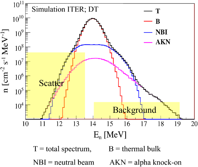

    

    Adopted from Ref. [25]

    Simulation of expected neutron emission spectral components in a 50:50 DT plasma of typical ITER conditions; injection energy of the deuterium NBI is 1 MeV. Red full line corresponds to thermal DT reactions, blue line to D beam-thermal T reactions, and magenta full line to the alpha knock-on effect. The estimated level of scattered neutrons and background are also indicated in yellow (Colour online).

  • Results should be reported with a time resolution down to ms. For the type of counting experiments that are typical for neutron diagnostics this means a requirement to accept and acquire data of MHz signal rates. In other words, the count rate capability of the system has to be high, in the MHz region.

  • For machine control and protection, information is required in real-time with down to ms time resolution: this means fast transfer rates from acquisition electronics to processing units as well as fast and robust data analysis.

• Interfacing can be an issue:

  • The size and weight of the neutron spectrometry systems are considerable.

  • The desire to place the systems close to the neutron source (i.e., the plasma), in order to maximize count rates, means that large and heavy components for radiation shielding are required.

  • Maintenance and replacement of components in positions close to the fusion source is a challenge.

  • A competition for “real estate” around the fusion device, where bulky neutron diagnostic systems, closely coupled and with “direct” lines-of-sight into the plasma, can be at a disadvantage.

Finally, it should be mentioned that the very high neutron rates expected in future high-performance fusion devices, such as ITER and DEMO, which are seen as problematic for many of today’s plasma diagnostics, are instead a great opportunity for neutron diagnostics of all types.

Review of Neutron Spectrometry Techniques: Compact Detectors

There is a quite broad range of techniques and detectors that can (and have been) used for fusion neutron spectroscopy [26, 27]: they span from small compact single detectors/monitors of a few kg to very specialized instrument systems of considerable weight (10’s of tons) and size (several m³). Some of the more common techniques are schematically depicted in Fig. 8.

Fig. 8

Schematics of the main neutron spectroscopy techniques discussed in this paper. Top left illustrates use of a hydrogenous scintillator, bottom left use of a diamond semiconductor, middle shows the two variants of the thin-foil proton recoil technique; right the time-of-flight technique

As can be seen in Fig. 8, many of the neutron detection techniques listed in “The Fusion Plasma as a Neutron Source: The Direct Emission” section have been tested and used in fusion. JET in particular has over the years had an ambitious program of neutron diagnostics, including, in particular, several different types of neutron spectrometers [26].

Scintillators with a large hydrogen content are often employed as neutron counters and also, in a more limited capacity at least for fusion, as spectrometers. The main mechanism for detection in this case is (n, p) elastic scattering. This subject is only briefly introduced here and more extensively covered in another paper in these proceedings (M. Cecconello); it will not be discussed further here. Here, instead, we will focus on a few other neutron measurement and spectroscopy techniques.

Example 1: Semiconductor Detectors; Diamonds (C)

Diamond is a very interesting detector material for fusion diagnostics [28, 29], primarily for neutron counting and spectroscopy, for a number of reasons:

• There are a number of useful nuclear reaction channels with neutrons, some providing charged particles (only) in the final state. This provides a reasonable efficiency and the possibility for spectroscopy;

• It is mechanically a very robust material, and chemically benign (non-toxic, resistant and inert to many chemicals, etc.);

• It can withstand high temperatures;

• It is allegedly very radiation hard;

• There is rapid progress in fabrication of synthetic, single crystal diamonds suitable for neutron spectroscopy through the Chemical Vapor Deposit method; quality and size of samples is improving.

For low energy neutrons (i.e., for fusion neutrons in D plasmas), there are two main reaction channels open:

• n + ¹²C → n + ¹²C (elastic),

• n + ¹²C → ¹³C* (n capture (γ))

At higher neutron energies, from about E_n > 5 MeV, several new reaction channels open up (available for fusion neutrons in DT plasmas):

• n + ¹²C → n′ + ¹²C* (Q = − 4.4 MeV)

• n + ¹²C → α + ⁹Be (Q = − 5.7 MeV)

• n + ¹²C → n′ + 3α (Q = − 7.3 MeV)

The cross sections for some of these reactions are shown in Fig. 9. As can be seen in the figure, the situation is rather complex, with many reaction channels open (depending on E_n), and in order to understand the response of a diamond detector one needs to know such cross sections in detail, both the excitation functions (dσ/dE; as shown in the figure) and the angular differential cross sections (dσ/dθ). In addition, detailed kinematics modeling of the reactions is required. A somewhat more complete table of the possible final state particles in n + ¹²C reactions is given in Table 1. As shown, for fusion relevant neutron energies, E_n < 20 MeV, there are at least 8 open reaction channels.

Fig. 9

Cross sections as function of neutron energy from the ENDF data library for some of the neutron induced reactions in diamond (¹²C). Included are the total cross section (n,tot), the cross section for leaving the ¹²C in its first excited state at 4.44 MeV and the cross section for the (n,a) reaction (suitable for neutron spectroscopy). Data from Ref. [30]

Table 1 Some of the final state particles in n + ¹²C reactions and their Q values

Characterization of an actual diamond detector with mono-energetic 20 MeV neutrons is shown in Fig. 10. Here, many of the reactions of Table 1 can be identified. In particular, the very favorable situation with the ¹²C(n,α)⁹Be reaction is evident. This reaction has the lowest Q value (Q = − 5.70 MeV) of all the channels with charge-only final states. The charged-only final state makes it well suited for spectroscopy, in particular of neutrons in DT plasmas, where the main direct emission is centered around E_n = 14 MeV. The energy of the final state particles, about 8.3 MeV for E_n = 14 MeV, is the highest for any charged-only channel, so the full-energy peak is well separated from the rest of the spectrum. Energy resolution of dE/E < 3% has been achieved with diamond detectors intended for use at fusion facilities [31].

Fig. 10

Adapted from Ref. [32]

Response of a diamond detector to mono-energetic neutrons of E_n = 20 MeV. Some of the structures in the spectrum are identified by their reaction channel and their Q value. Peaked structures typically correspond to charged-only final states, while broad structures correspond to final states with (at least) one neutral particle (here neutron).

Another beneficial property in this context is the fairly “flat” cross section for E_n > 9 MeV, simplifying the interpretation of data. A slight drawback of the diamond detector is the rather low ratio of good events in the (n,α) peak compared to the rest of the spectrum. As seen from Fig. 9, at E_n = 14 MeV this is on the level of a few percent. Even though the (n,α) events stand out clearly in the spectrum, all the other reaction channels will put a load on the detector and acquisition electronics, limiting the count rate capability (of good counts in the (n,α) peak) to below 100 kHz or so. This, in turn, will limit the achievable time resolution for physics results.

In order to analyze data from a diamond detector the response of the detector to neutrons in a broad range of energies is required. Such a response function, connecting the measured quantity of the instrument with the neutron energy, is often constructed from a mixture of data from measurements (such as those in Fig. 10) and simulations. The simulation model is tuned to reproduce the experimental data, and is necessary in order to supplement the often limited number of measurements at different neutron energies. The measurements will put constraints on the modeling, and a good coverage of experimental data over the energy region of interest helps improve the modeling. The primary use of diamonds would be as neutron spectrometers in DT plasmas, which would suggest a detailed characterization of the response in the region 10 < E_n < 20 MeV. Such a characterization is described in Ref. [32].

Even though the charged-only channels, in particular the (n,α) reaction, are best suited for spectroscopy, it should be mentioned that also n-¹²C elastic scattering can be used, in a manner similar to that in scintillators (where n–p elastic scattering is the primary reaction). This opens up for the use of diamonds also in D plasmas, something that has indeed been tested at JET [33]. Figure 11 shows results for a diamond used at JET in DD operations, where data from a set of 45 NBI heated discharges were summed to produce the pulse height spectrum. The calculated response for a number of mono-energies is shown in the top panel and the measured data, together with a component fit, at the bottom. A good agreement between modeling and data is obtained, indicating that physics results pertaining to the neutron spectrum can be extracted. An obvious drawback is the rather low neutron rate and efficiency of the detector, which makes it necessary to sum many discharges in order to obtain sufficient statistics to perform the analysis.

Fig. 11

(Top) Ideal response of a diamond detector to low energy mono-energetic neutrons in the range 2 < E_n < 3 MeV through n-¹²C elastic scattering. (Bottom) Experimental data from a diamond detector installed at JET (points with error bars). A model response has been fitted to the data, partly based on the calculated response functions in the top panel. The best fit is shown in magenta and includes components corresponding to Direct neutron emission (brown), Scattered neutrons (green), gamma rays (dark blue), and a calibration alpha source (light blue). From [33] (Colour online)

Diamond detectors are an active line of research and development in fusion neutron diagnostics. At JET, for example, two sets of diamond detectors are currently installed, one single crystal detector in a tangential line-of-sight, and a pixelated, 3 × 4 matrix, of 12 crystals in a radial, vertical LOS. The latter is shown in Fig. 12.

Fig. 12

(Left) Schematic design of the 3 × 4 pixel diamond detector installed in the Roof laboratory of JET. (Right) Photo of the diamond detector before installation. From [34]

In summary, diamond detectors seem to offer a robust technique for neutron spectroscopy in particular for DT operations. However, the experimental use at high performance fusion devices is still somewhat limited, and some issues with diamond detectors remain to be studied:

• The low fraction of useful counts in the (n,α) peak, corresponding to a few % of the total load, means that the detector “efficiency” for useful counts is low. Thus, very high total count rates will be required and the count rate capability for neutrons and the influence of pile up at high rates must be studied.

• In diamonds produced with natural abundance carbon, about 1% of the nuclei will be ¹³C. This means that the ¹³C(n,α) reaction can disturb measurements of weak neutron spectral components.

• A “polarization effect” has been observed, meaning a degradation of the output pulse height over time. The cause of this effect is at present not fully understood, and should be investigated further. The effect can be mitigated by reversing the detector bias after some time of exposure.

• The main production technique for artificial diamonds through the CVD process has limits when it comes to the dimensions of spectroscopy-grade crystals: at present the limit is a few tens of mm² in area, and a thickness up to 1 mm. Increased dimensions, in particular thickness, would be important to increase the efficiency of the detectors.

• The radiation hardness properties of diamond detector assemblies should be investigated further. Recent results have indicated issues, possibly related to the contacting of the detectors [35].

Example 2: In-Organic Scintillators for n Spectroscopy—CLYC: Cs₂LiYCl₆:Ce Crystals

A recent development with potential for neutron measurements, also fast neutron spectroscopy, at fusion facilities is the so called CLYC scintillator material [36, 37]. The chemical composition is Cs₂LiYCl₆:Ce, where the elements of interest for neutron induced reactions are mainly Li and Cl. Even though the potential for high-performance neutron spectroscopy might be somewhat limited, the material would offer interesting possibilities of measurements in mixed radiation fields of thermal and fast neutrons, in combination with a strong gamma component.

The reactions of interest for neutron measurements are:

• ⁶Li(n,α)³H with a Q = 4.8 MeV, i.e., there is no threshold for this reaction, and it is therefore well suited for thermal neutron measurements. In principle, in view of the charged-only final state, this channel could be used for neutron spectroscopy, although the very strong thermal cross section tends to overshadow the effects of fast neutrons.

• ⁷Li(n,αn)³H with a Q = − 2.5 MeV, i.e., a threshold reaction, thereby sensitive to counting of fast neutrons. However, the 3-body final state, involving a neutron, does not make this reaction channel suitable for spectroscopy.

• ³⁵Cl(n,p)³⁵S with a Q = 0.61 MeV. This charged-only reaction channel has a potential for neutron spectroscopy that could be explored.

Some of the attractive properties of CLYC are:

• A good energy resolution of about dE/E ~ 4% for gammas at E_γ = 660 keV. This is worse than semi-conductor detectors, such as diamonds, but on par with many other recently developed in-organic scintillators, such as LaBr₃ and CeBr₃ based detectors.

• The pulse shape response to neutrons and gammas is quite different, as shown in Fig. 13, which opens up for excellent neutron-gamma event separation through Pulse Shape Discrimination analysis techniques.

  Fig. 13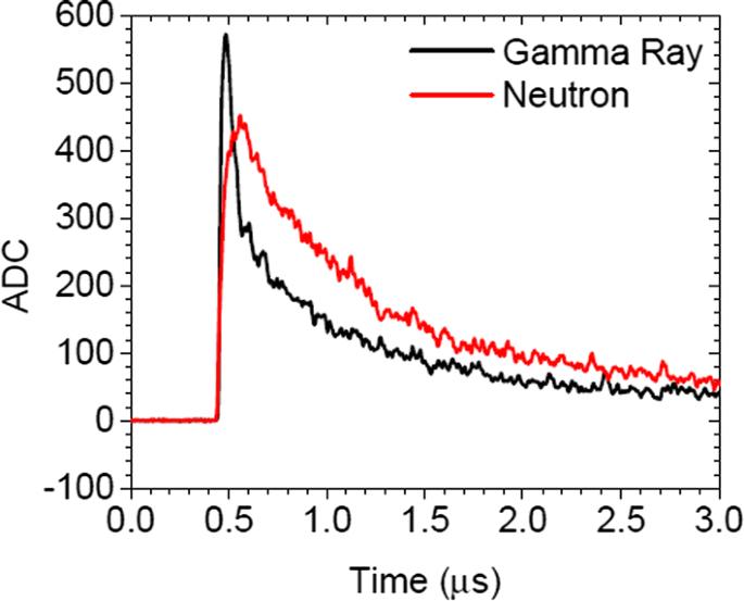

  

  Example of the difference in detector pulse shapes between neutron and gamma induced events in a CLYC detector

• There is a possibility to tailor-suit the detector by selective enrichment of the Lithium isotopes:

  • enriching in ⁶Li increases the sensitivity for thermal neutron counting

  • enriching in ⁷Li improves the performance for fast neutron counting

Figure 14 illustrates the possibilities to separate different reaction channels by pulse shape analysis (Pulse Shape Discrimination, PSD). As can be seen, the neutron induced reactions are well separated from the gamma reactions.

Fig. 14

Example of the use of a CLYC detector in a mixed field of gammas and neutrons. (left) Separation of events (reaction channels) through pulse shape discrimination (PSD). The neutron-induced reactions on ³⁵Cl and ⁶Li are indicated. (right) Projection on the pulse height axis of the neutron-induced events in the red rectangles. From Ref. [37]

Several issues remain for this material to be considered as a resource in fusion diagnostics:

• As shown in Fig. 13, the light decay constant is of the order μs, thereby restricting the count rate capability if pile up at high rates is to be avoided.

• In a mixed field of gammas and neutrons, as is often the case in fusion, the reactions involving neutrons are only a small fraction of the signals generated in the detector. The fraction of events useful in neutron counting or for neutron spectroscopy is small.

• The response of the detector to neutrons at different energies must be measured in detail, to investigate if the potential for spectroscopy can be fulfilled.

• The technique should be tested at a high-performance fusion facility to assess its potential in fusion neutron diagnostics.

Advanced Neutron Spectrometry: n–p Elastic Scattering

In this and the following sections we will focus on two techniques used in more specialized, designed neutron spectroscopy systems: the time-of-flight (TOF) technique and the thin foil proton recoil (TPR) technique. The design of these systems allows their performance to be adjusted to the needs of the specific measurement situation when it comes to the main system characteristics like energy resolution, detection efficiency and count rate capability. Still there are inherent limitations with the techniques that must be known and taken into account in any real implementation at a fusion device. As an introduction to this discussion we need to take a look at the basic reaction of neutron elastic scattering on hydrogen (protons), as this is the basis for the signals detected in the systems.

Elastic Scattering H(n,n)H

The basic reaction utilized in both the TPR and (forward) TOF techniques is neutron elastic scattering on hydrogen: n + p → n_R + p_R, where R indicates the recoiling particles after the interaction. Neutron elastic (nuclear) scattering on hydrogen (i.e., protons in the target material) has several advantages:

• The reaction has a high and well known (uncertainties of single%) differential cross section, both regarding dσ/dE and dσ/dθ, in fusion relevant neutron energies, E_n < 20 MeV. This opens up the possibility for good absolute measurements, if other experimental parameters are known to a similar level of precision. See Fig. 15.

  Fig. 15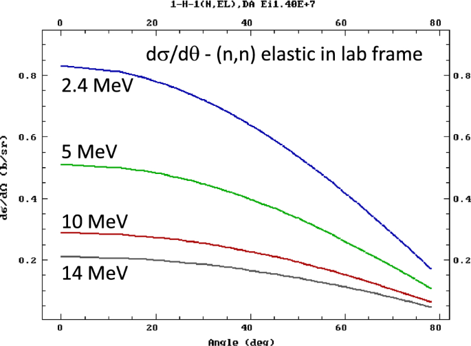

  

  Adapted from [30]

  The differential (dσ/dθ) cross section for elastic nuclear H(n,n)H scattering in the laboratory reference frame for a number of selected incoming neutron energies. Kinematically, the highest possible scattering angle is 90° (assuming m_n = m_p).

• The differential cross section is close to isotropic in the Center-of-Mass system for E_n < 20 MeV, although a slight anisotropy in the backward (CM) direction starts to develop for E_n > 10 MeV. This means a corresponding slightly enhanced probability for protons scattered into the forward direction, and can be of relevance in some cases, in particular for absolute estimates. See Fig. 16 [30].

  Fig. 16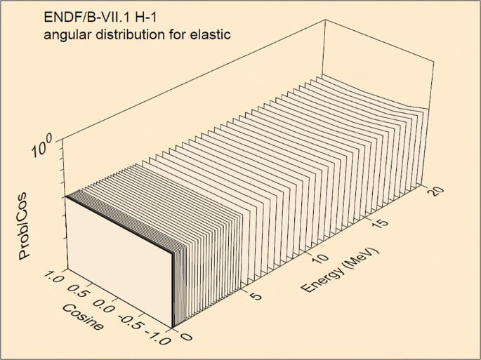

  

  The differential (dσ/d(cosθ)) cross section for elastic nuclear H(n,n)H scattering in the CM frame for 0 < E_n < 20 MeV. From [38]

• There exist a range of suitable hydrogenous material, suitable both for active measurements (such as scintillators) and as self-supporting, passive scattering materials (plastic foils).

• The kinematics of n–p elastic scattering for E_n < 20 MeV is quite simple: no excited states of the outgoing particles exists and the neutron energy is well below any threshold for production of secondary particles.

• The kinematics of neutron elastic scattering on nuclei (Eq. 9) shows that scattering on Hydrogen gives the Hydrogen nucleus (proton) the highest possible charged recoil energy of any nucleus. For head on collisions (θ_p = 0), practically the full neutron energy can be transferred to the recoil proton, E_p = E_n (ignoring the small neutron–proton mass difference):

  $$ E_{r} = \frac{4A}{{\left( {1 + A} \right)^{2} }}\left( {\cos^{2} \theta } \right)E_{n} $$

  (9)

Here E_r is the energy of the recoiling nucleus, A is the atomic mass number of that nucleus, θ is the neutron scattering angle in the lab frame, with θ = 0 for head-on collisions.

One can identify three cases for using the p(n,n)p (elastic) reaction for neutron measurements:

• 1. Only look at the recoil protons: allow protons at ANY scattering angle; measure the energy of the recoil protons. This is used in most scintillators, like the liquid NE213 scintillator. (See paper by M.Cecconello in these proceedings.)

• 2. Only look at the recoil protons: passively allow protons only in a restricted angular interval; measure the energy of the recoil protons. This is used in the TPR technique, and has been implemented in the MPR/MPRu spectrometer at JET and suggested for ITER, as further discussed in Sect. 11 below.

• 3. Measure the recoil proton (energy and time) in an initial n–p scattering, follow the neutron, measure the proton (energy and time) in second n–p scattering: this is used in the TOF technique and implemented for example in the TOFOR spectrometer at JET.

In the following sections we will take a closer look at diagnostic systems based on points 2 and 3 above.

Time of Flight Systems

The neutron time-of-flight technique is based on a simple concept: measure the time t_TOF for the neutron to traverse a known distance L. From this, calculate the velocity, v = L/t_TOF, and finally determine the (non-relativistic) neutron energy according to Eq. 10:

$$ E_{{n^{{\prime }} }} = \frac{1}{2}m_{n} \nu_{{n^{{\prime }} }}^{2} = \frac{1}{2}m_{n} \left( {L\frac{{}}{{t_{\text{TOF}} }}} \right)^{2} $$

(10)

Here, m_n is the neutron mass.

In some applications, a suitable time reference exists for the time measurement, like the RF system of an accelerator. In high-performance magnetic confinement fusion experiments, however, where plasma discharges can extend for several seconds, no such useful time reference exists. Instead, a neutron double scattering configuration is used, where the same neutron is detected in two (sets of) detectors, here called S1 for the first (start) detector and S2 for the second (stop) detector, and the distance and time between these detectors define the velocity of the scattered neutron. The principle of the technique is shown in Fig. 17(left). Note that in both S1 and S2 detectors, the actual measured signal is due to the recoils protons, according to the discussion in the previous section. In order to achieve sufficient (proton) signal amplitude in the elastic scattering in S1, the S2 coincidence detector is placed at some angle, α, with respect to the incoming neutrons from the plasma. The incoming neutrons are normally shaped into a “beam” by suitable collimation between the diagnostic and the plasma, as shown previously in Fig. 4.

Fig. 17

(Left) The principle of the neutron double scattering technique used for fusion neutron time-of-flight measurements. (Right) Geometry for the concept of constant time-of-flight sphere. Also, the tilting of the S2 detector as used in the TOFOR implementation at JET is indicated. See text for details

In principle, one can envisage both forward scattering and backward scattering TOF systems. The latter would then depend on a primary scatter (in S1) on a nucleus heavier than hydrogen (proton). Such a possibility is offered by using a deuterated scintillator as S1. Such a solution is considered for the ITER High Resolution Neutron Spectrometer system presented later in this paper. However, in what follows we will mainly discuss the forward scattering TOF technique.

In the double scattering configuration, the energy of the scattered neutron, E_n′, is related to that of the primary incident neutron, E_n, through the scattering angle α:

$$ E_{{n^{\prime } }} = \, E_{n} \cos^{2} (\alpha ) $$

(11)

From geometric considerations (Fig. 17(right)), one can conclude that the distance L between any two points on a circle connecting the center of S1 and the center of S2 can be written:

$$ L^{2} = 2R^{2} \left( {1 - \cos (\pi - 2\alpha )} \right) = 4R^{2} \cos^{2} (\alpha ). $$

(12)

Combining the three Eqs. 10, 11, 12 finally yields an expression for the energy of the primary, incoming neutron, E_n, that is independent of both the distance L and the scattering angle α, and only dependent on the (fixed) radius R and the measured time-of-flight:

$$ E_{n} = \, 2m_{n} R^{2} /t_{TOF}^{2} $$

(13)

This is the basis for the “constant time of flight sphere” concept, which states that under the assumption of elastic n–p scattering and as long as the secondary detectors, S2, are placed on a sphere of radius R, the energy of the incoming neutron is determined solely by the measured time-of-flight.

Equation 13 gives some important information on how we should design our TOF spectrometer. By differentiating the expression we obtain the expected uncertainty in the energy measurement, i.e., the energy resolution, as a function of the experimental parameters R and t_TOF, as given in Eq. 14:

$$ \frac{{dE_{n} }}{{E_{n} }} = \sqrt {\left( {2\frac{dR}{R}} \right)^{2} + \left( {2\frac{dt}{{t_{TOF} }}} \right)^{2} } $$

(14)

In the design of the spectrometer, one often strives for a certain maximum energy resolution, and an analysis of the contributions in Eq. 14 can help in that work.

Here it is important to note that the uncertainty, dR, in the radius R includes two components: first the uncertainty in the installed positions of the S1 and S2 detectors, and second, the additional uncertainty in the actual interaction positions within the finite thickness of the S1 and S2 detectors. While the former uncertainty is a common, systematic uncertainty for all measurements, the latter component is a true random uncertainty.

Also note that the dt used here means the uncertainty in the intrinsic time determination, and not the width of the measured time-of-flight peak (which is actually directly correlated to dE/E). This dt is given by uncertainties in the timing electronics, in the time pick-off method, in the statistical variations in the signal pulse shapes etc. In many cases dR ≫ dt and the expression for the energy resolution reduces to dE/E = 2dR/R, i.e., the resolution can be estimated from geometry alone. Furthermore, the (systematic) uncertainty in the determination of the positions of S1, S2 can be assumed to be of the order mm or better. This means that in many cases, it is the detector thickness of S1, S2 that will be the main contribution to the energy resolution.

As indicated above, when real measurement data is available, the energy resolution is given by the observed width and position of the measured time-of-flight distribution (peak), as given by (dE/E)_meas = (2dt_TOF/t_TOF)_meas. Here dt_TOF is the full width at half maximum of the measured time-of-flight peak, and t_TOF the mean time-of-flight.

Several time-of-flight spectrometers have been used in fusion research over the year. Two recent examples are the TOFOR [39,40,41] and TOFED [42, 43] spectrometers, installed at JET and EAST, respectively. Here we will give a more detailed description of the TOFOR spectrometer [44].

The TOFOR spectrometer at JET was installed in 2005 and was built based on the following design drivers [adopted from Ref. 45]:

• Optimize the design for D plasma measurements (E_n ≈ 2.5 MeV).

• Strive for an energy resolution corresponding to a T_i ≈ 4 keV, i.e., dE/E ≈ 6.6%.

• The spectrometer should have a high count rate capability, with a maximum capacity of about C_cap ≈ 500 kHz.

• It should be a simple, robust design, in particular including a large area S2 for high efficiency.

The design resulted in a system of compact dimensions, nicely fitting in the designated position in the JET roof laboratory, with α = 30degr and L = 1.22 m, giving an estimated average t_TOF (E_n = 2.45 MeV) = 65 ns.

It was decided to base the design on fast plastic scintillator detectors coupled to photo-multiplier (PM) tubes. There were several reasons for this choice:

• Plastic scintillator is a hydrogenous material with suitable and well-known mechanical and detector properties. The composition is basically (CH)_n thus providing ample scattering centers (protons) for (n,p) elastic scattering.

• Fast plastic means fast signal rise times which provide a good experimental situation for precise timing measurement.

• Plastic scintillators are robust, machineable, and have a good track record in nuclear and particle physics experiments.

TOFOR is composed of two sets of detectors, as depicted in Fig. 18(left):

Fig. 18

(Left) Schematic drawing of TOFOR at JET. The neutron flux from the tokamak is shaped into a “beam” indicated by a broad, light blue arrow though the center of the figure. Primary neutrons, n, are scattered, n′, towards S2, where a second scattering might happen, giving a scattered neutron n″. The 5 scintillators of the S1 stack are placed in the center of the lower light blue ring. The 32 S2 detectors are indicated in medium blue, forming an “umbrella” symmetrically around the neutron beam. Dark blue, orange and brown are support structures. (Right) Geometry of the installation of TOFOR in the JET roof laboratory. The TOFOR is not to scale. The red cone indicates the instrumental field-of-view (Colour online)

• i. A stack of five S1 “start” detectors, each a disk of radius R_S1 = 20 mm and thickness t_S1 = 5 mm, making a total material thickness of 25 mm and a geometrical thickness of 27 mm, allowing for 0.5 mm distance between the disks in the stack. Dividing the S1 into several detectors improves the C_cap, since pulse time properties, PM tube and acquisition electronics set a limit for the count rate in each individual detector channel at about 1 MHz.

• ii. A set of 32 S2 “stop” detectors of “paddle” shape, each 350 mm long and 15 mm thick. The S2:s form an “umbrella” like structure placed symmetrically around the symmetry axis of the instrument, which coincides with the collimated neutron beam.

The installation at JET is schematically depicted in Fig. 18(right). TOFOR is installed in the roof laboratory at JET, about 19 m from the center of the plasma and with a line-of-sight going through the center of the plasma (note, the size of TOFOR is not to scale). The collimation is integrated in the roof laboratory floor which is about 2 m thick and also acts as radiation shield.

The geometry of the S1 and S2 detectors was determined in a performance optimization simulation study, where the thickness of the detectors was varied in order to find the combination with the highest possible efficiency for a selected energy resolution. The target energy resolution was set to 5.8% and the results from the optimization are shown in Fig. 19. Note that, in general, there is a reciprocal relationship between resolution and efficiency, such that a higher efficiency leads to a worse resolution. The red dot indicates the selected optimal geometry with t_S1 = 25 mm (5 × 5 mm) and t_S2 = 15 mm. This combination actually has a slightly better resolution than the target (dE/E < 5.8%) for an efficiency of slightly higher than 0.12 cm² (area efficiency).

Fig. 19

Adapted from [39]

Results from GEANT simulations of TOFOR’s performance in a study to optimize the thickness of the S1 and S2 detectors. Full lines indicate efficiency contours in units of (cm²), i.e., including the S1 detector area. Dashed lines indicate FWHM energy resolution contours in units of (%). The red dot indicates the selected geometry for the TOFOR design.

Since the S2 detectors are fairly large, and have their PM tubes attached at the lower end, they were tilted away from the constant time of flight sphere in a manner shown in Fig. 17(right). The tilt is such that neutrons at the upper tip, far from the PM tube, will reach the detector slightly before neutrons at the lower tip, close to the PM tube. This is to partly compensate for the slightly longer light transmission time through the length of the S2 detectors for neutrons interacting at the far end (with respect to the PM tube) compared to those interacting at the near end.

Combining the effects of the geometry, tilting of S2, and electronics, an overall energy resolution of about dE/E ≈ 7% was achieved for TOFOR for E_n = 2.5 MeV. Due to the choice to optimize TOFOR for D plasmas, the performance in DT plasmas (E_n = 14 MeV) will be somewhat reduced.

The original TOFOR installation included digital electronics that provided free-running time stamps (only) of all eligible events (i.e., events in the detectors above a set pulse-height discrimination threshold). As shown in Fig. 20(top), time-of-flight values were determined by selecting a signal in S2 (which is exposed to considerable lower rates than the in-beam S1) and calculating the time difference to all S1 signals in a specific time window, often taken to be ± 200 ns. In the example of the figure, four different S1 events are eligible to form a t_TOF with this specific S2 time stamp. Without pulse height information, all interactions in S1 (within the time window) are eligible as a valid S1–S2 coincidence, although in reality only one of the S1 interactions is actually induced by the same neutron that later interacted in S2. This makes the original TOFOR system sensitive to so called random (accidental) coincidences, i.e., t_TOF values formed between uncorrelated neutrons. The situation is particularly severe at high count rates, since the signal count rate (true coincidences) scales as S_true ∝ Y_n, while the random background scales as S_false ∝ Y ²_n , where Y_n is the neutron rate from the plasma. With the TOFOR type of electronics, at some neutron rate the false (random) signals will completely overshadow the true signals, making the system useless as a spectrometer.

Fig. 20

Illustration of the way the time-of-flight is determined, also illustrating the are difference between original TOFOR time stamping electronics (top) and the upgrade ToFu system capability (bottom). With ToFu, correlation between time-of-flight and energy (pulse height) makes it possible to discard (red crosses) certain S1–S2 combinations as invalid (Colour online)

The problem can be partly overcome by measuring correlated time and energy (pulse height) information. The original TOFOR electronics did not allow for this, and therefore an electronics upgrade program for TOFOR has been initiated, dubbed ToFu [46, 47]. The main element of the upgrade program is to replace the original TOFOR time stamping (only) electronics with state-of-the-art waveform digitizers (1 GHz sampling rate, 12–14 bit amplitude resolution, fast data transfers, etc.). This allows making more strict selection of eligible S1 “candidates” for each S2 signal, as shown in Fig. 20(bottom): some combinations of energy and time-of-flight simply do not comply with the requirement of elastic n–p scattering.

The ToFu upgrade program is well under way, and described in some detail in for example Ref. [47]. Figure 21 illustrates the new capabilities offered with ToFu. Figure 21a, b show the possibility to plot the data in a two dimensional histogram, with energy versus time. The red lines in (a) indicate the kinematic correlations (energy-time) for eligible events in S1 directed towards the tips of the S2 detectors; events outside of these lines are NOT eligible single n–p elastic scattering events in S1 and can be discarded. In S2, panel (b), only an upper level can be set, indicated by the single red line. Still, all events above this line can be discarded. The process of applying these time-energy correlations is dubbed “kinematic cuts”.

Fig. 21

Illustration of the improved background reduction offered with the ToFu electronics upgrade. a Correlation between t_TOF and energy deposition in the S1 detector, red lines indicate the allowed region for n–p elastic kinematics, b correlation between t_TOF and energy deposition in the S2, red line indicate the upper E_S2 threshold; c projection of the t_TOF distribution in (a) (or b) as in the original TOFOR (no kinematic cuts), blue line is for full data set, red line is the estimated level of random coincidence background, green line is background subtracted data; d projection of the t_TOF distribution including kinematic cuts, blue line is all events that pass the cuts, red line is estimated random background, green line is background subtracted data. From [47] (Colour online)

Figure 21 panels (c) and (d) show the projections of the recorded events in panels (a) and (b) without (panel c) and with (panel d) kinematic cuts. Note that panels (a) and (b) both include the same “coincident” events, so projections of panels (a) and (b) on the time-of-flight axis, without cuts, will be exactly the same, in each case giving the blue line in panel (c). Panel (c) illustrates the background subtraction possible with the original TOFOR electronics: the level of random coincidences for the data set under study was determined from a region on the negative time-of-flight side of the spectrum. This level was then subtracted from the data over the whole spectrum to find a representation of the true coincidences as shown in the green curve in panel (c) (or to be more precise, the level of random coincidences was included as a component in the physics analysis of the data).

With the new ToFu electronics, the kinematics cuts (red lines) are applied to panels (a) and (b) and only those events passing both cuts are plotted in panel (d) (blue line). The shape of the spectrum for times-of-flight formed with negative values can again be used (now mirrored around t_TOF = 0) to estimate the influence of the random background. The final selection of eligible events is shown in the green curve in panel (d).

There are a number of observations to be made when comparing the green curves of panels (c) and (d): (i) the gamma peak at t_TOF = 4 ns has completely disappeared in panel (d). This is as expected, since there should be no possibility that gamma interactions pass as single scattering elastic neutron events. The high t_TOF tail is much reduced in panel (d) compared to panel (c). This gives improved possibilities to understand the influence of scattered neutrons in all plasmas, and in particular improves the prospect of measuring 2.5 MeV neutrons in a strong background of 14 MeV neutrons, as will be the situation in future JET DT campaigns. Finally, but not so clear from this figure, the quality (in terms of statistical uncertainty) of the 14 MeV peak at 27 ns has improved considerably in panel (d) compared to panel (c).

The work on the ToFu upgrade is still ongoing, but it is already now clear that it will improve the TOFOR system data quality in both D and DT plasma operations.

Thin Foil Proton Recoil Systems

The thin foil proton recoil (TPR) technique is also based on elastic n–p scattering. Contrary to the TOF technique, in a TPR only a single elastic n–p scattering is used and no further measurement of the scattered neutron is done. The technique is based on measuring the energy of the scattered proton in a restricted angular range, preferably in the forward direction.

This leads to an important design restriction, namely that the primary proton “radiator” must be thin, in order to avoid a large and unknown proton energy loss. In practice, thin self-supporting CH₂ foils are used for the primary scattering. However, an advantage with the method is that these foils can be completely passive and any active signal measurements are done outside of the collimated neutron beam. This decoupling of the n–p scattering from the actual measurement facilitates the design and makes it, in principle, possible to shield the active detectors to any desired level. Thus, by careful instrumental design, this technique has the potential to provide excellent signal to background ratios, thereby allowing for measurements of very weak components in the neutron spectrum.

The two main implementations of the TPR technique are schematically shown in Fig. 22, where TPR here means the specific case with a proton energy-resolving detector placed at an angle θ out of the neutron beam. MPR stands for Magnetic Proton Recoil, and is further discussed below. The basic principle in both cases is: (i) neutrons from the fusion plasma are collimated into a neutron beam, (ii) the beam neutrons intersect a thin hydrogenous foil, (iii) some of the neutrons undergo elastic n–p scattering in the foil, (iv) the recoil proton is allowed to exit the foil and its energy is measured at some angle (in the forward direction).

Fig. 22

Schematic illustration of the TPR/MPR neutron spectroscopy technique. TPR stands for Thin-foil Proton Recoil, MPR for Magnetic Proton Recoil

There are several advantages of selecting the protons in the forward direction:

• The energy of the recoil proton is the highest possible, thereby facilitating its detection and separation from background.

• The variation in proton energy is the smallest over a specified angular range (Fig. 23).

  Fig. 23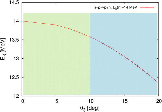

  

  Adapted from [48]

  Kinematics of elastic n–p scattering for incoming neutrons of E_n = 14 MeV. The recoil proton energy as function of proton angle is shown. The green region roughly corresponds to the situation in the MPR, the blue region to the TPR (Colour online).

• The spread in proton energy loss for a specific foil thickness is minimized.

All the above points help to improve the performance and energy resolution of the system. The use of thin foils also improves the resolution, but decreases the efficiency. Thus, the TPR/MPR technique is best suited for high-performance DT operations where neutron rates are high, and the low efficiency is less of a limitation.

Since charged particles are tracked in the TPR/MPR, energy loss outside of the scattering foil and the active detectors should be avoided. Therefore, the space between the foil and the detector(s) should be evacuated. However, the required vacuum levels are moderate, and levels of the order p < 10⁻³ mbar will normally suffice, putting rather relaxed demands on the vacuum system.

The MPR Spectrometer at JET

An instrument based on the MPR technique was installed at JET in the Torus Hall some 8 m from the plasma center in 1996 [49,50,51] and has provided a wealth of neutron spectrometry data. Some early results can be found in e.g. Refs [10, 49, 52, 53]. This technique employs a magnetic spectrometer to separate the selected forward-scattered protons according to their momentum (energy), as given by the cyclotron equation: Bρ = p/q, where B is the applied magnetic field, ρ is the bending radius, p is the particle momentum and q is the charge of the particle. This means an approximate bending radius of ρ=0.7 m for E_p = 14 MeV and B = 1 T. The MPR instrument at JET is depicted in Fig. 24. The magnetic spectrometer is of a traditional nuclear physics design, using ordinary magnetic materials. It is thus rather bulky (several m³), heavy (about 20 tons) and requires considerable power to operate. The active detection system is a 32 element fast plastic scintillator hodoscope, placed approximately in the focal plane of the magnetic system about 1.5 m from the neutron beam (n–p scattering foil). This allows for a very high count rate capability of the spectrometer, of several MHz signal count rate, and very good signal-to-background ratios.

Fig. 24

Schematic drawings of the MPR/MPRu spectrometer at JET. (top) A cut side view through the center of the system, showing the concrete shield, the magnetic spectrometer system (split in two “dipoles”), the neutron collimator, the scintillator hodoscope etc. (bottom) A more detailed view of the magnetic and detector systems. From [54]

Due to its position in the JET Torus Hall, close to the plasma, a rather substantial radiation shield is required around the spectrometer. As seen in the figure, the instrument is enclosed in a concrete “bunker” weighing about 65 tons.

The MPR has been designed to provide very good resolution of 14 MeV neutrons, corresponding to dE/E = 2.5% for the optimized setting. There are three main contributions to the energy resolution of the MPR:

• Energy loss in the n–p scattering foil, dE_t. The scattering reaction can take place at any (random) point within the foil, and the outgoing recoil proton will have to traverse a distance in the foil, ranging approximately 0 < L < t_foil (somewhat adjusted for the outgoing proton direction). This inflicts an unknown energy loss to the proton.

• n–p scattering kinematics, dE_k. Due to the finite acceptance angle of outgoing protons, and the divergence of the neutron beam at the foil, n–p elastic scattering kinematics give a range of outgoing proton energies even for a mono-energetic incoming neutron.

• Spectrometer ion optics, dE_o. The finite area of the scattering foil (10 cm²) and the properties of the magnetic system give a spread in proton positions at the hodoscope, even for mono-energetic neutrons. The finite width of the hodoscope detectors also add to this contribution.

In an optimized configuration, the three contributions described above should be matched and add about 200 keV each; the final resolution is obtained by adding the individual contributions in quadrature.

The MPR technique allows for a flexible system, and this has to some degree been implemented at JET. Thus, the magnetic spectrometer B-field can be varied in the range 0 < B < 1.4 T, there are several scattering foils available in a carousel-like arrangement, and there are several apertures for the recoil protons to enter the magnetic system. This makes it possible to combine different settings in order to obtain the best performance for a specific measurement situation: thicker foils and larger proton apertures give higher efficiency, but poorer energy resolution. Alternatively, thin foils and small proton apertures improves the resolution at the expense of detection efficiency.

A major upgrade of the original MPR was undertaken in 2005 (MPRu) [51], where the original 37-scintillator hodoscope was replaced with a 32-element system composed of so called phoswich scintillators. These detectors combine two scintillator materials of slightly different timing properties, thereby allowing for a better background discrimination. In order to reduce the background further, a layer of Gadolinium-based paint has been applied to certain areas of the spectrometer. This should help to prevent some of the thermal neutrons from entering the region close to the detectors, thereby reducing the gamma background due to neutron-capture reactions at the detector location.

The MPR/MPRu operated successfully in the JET major DT campaign in 1997 and also in the more restricted trace tritium campaign in 2003. It will be the main 14-MeV neutron spectrometer in any upcoming JET DT campaigns, as those presently planned for 2019–2020. Some results from the MPR are given in Refs [54,55,56].

The Non-Magnetic TPR Technique

The principle of the non-magnetic thin foil proton recoil technique [57, 58] is shown in Fig. 25. As in all fusion neutron spectrometers, the neutron flux onto the instrument is shaped into a beam by suitable collimators. As in the MPR, the neutron beam intersects a thin hydrogenous foil where some neutrons undergo n–p elastic scattering. The recoil protons are measured in a (set of) energy resolving detector(s) placed some distance L away from the scattering foil. A suitable aperture in the detector allows the neutron beam to pass through without directly interacting with the detectors.

Fig. 25

Schematic drawings of a non-magnetic TPR system. Elastic n–p scattering takes place in the polyethylene (CH₂) foil, a set of two annular detectors to measure the energy of the outgoing recoil proton is placed at a distance L from the foil. The front detector is thin enough to allow protons above a certain minimum energy to pass through to the back detector which is thick enough to completely stop protons up to a certain maximum energy. From [59]

The system in the figure is equipped with two detectors for proton energy measurements, in a ∆E–E configuration. This two-detector configuration helps to reduce background, which mainly will be due to neutrons from the collimated beam, scattered towards the active detector surface. For fusion neutron applications (DT operations), the combined thickness of the two detectors should be sufficient to fully stop protons up to E_max = 18–20 MeV. The active detector area covers a proton scattering angle of θ ± Δθ. In order to keep the resolution within the desired range, i.e., about 2.5% as in the MPR case, while simultaneously providing an efficiency high enough to provide time-resolved measurements, the annular ΔE-E might require some radial segmentation. It is possible to increase the efficiency further by placing several TPR systems in tandem. This is possible since the very thin foils used for the n–p scattering leave the passing neutron beam almost undisturbed.

Possible choices for detectors for the TPR are high-performance scintillators (e.g., YAP) or semiconductor detectors. In particular segmented Si strip detectors are an attractive choice, since there is a large experience base with such detectors in the nuclear and high energy physics communities. The required total Si thickness for stopping neutrons of E_n < 20 MeV would be about 2 mm. Commercial, annular, segmented Si detectors of such dimensions exist (t_ΔE = 0.5 mm, t_E = 1.5 mm) and are well-suited for a TPR application.

The resolution of the system will mainly depend on the thickness and radius of the foil, the angular range of the recoil protons and the intrinsic resolution of the energy-resolving detectors. As in the MPR case, a flexible system can be set up where a number of different pre-defined foils (of different thickness) can be selected, and the distance between foil and detectors varied.

In a study similar to that previously shown for the TOF technique, an optimization of the performance of the TPR can be performed [59]. In Fig. 26 the results from such a study are shown, where the efficiency (ε) and energy resolution were studied as function of the geometrical parameters of the system; here foil thickness, f, and distance between foil and detector, L. Two cases are shown, one where the detector segmentation has been used (Case 2; lettered results) and one without segmentation (Case 1; numbered points). Clearly the segmented solution gives a higher efficiency and more compact design, although at the cost of a more elaborate and expensive data acquisition system, in order to equip all segments with their own electronics read-out. Still, the performance (ε = 3·10⁻⁵, dE/E = 4.5%) and geometry of the system is quite attractive for neutron spectroscopy at high-performance devices such as ITER, although the system as shown here has not yet been tested at a real high-performance fusion facility.

Fig. 26

Results of an optimization study of a Thin Foil Proton recoil system for ITER. Case 1 (numbered points) is for a non-segmented detector, case 2 (lettered points) for a segmented one. (Left) Scatter plot of the values of Resolution and Efficiency for the selected geometrical configurations. The blue shaded area indicates the acceptable range of resolution values. (Right) The geometry for the evaluated geometrical configurations in terms of foil thickness, f, and distance between foil and dE detector, L. From [59] (Colour online)

Proposed High Resolution Neutron Spectrometer System for ITER

ITER has several neutron systems planned; some have been decided for full implementation while others are only developed to a conceptual level at this stage. Neutron spectroscopy on ITER falls in the latter category of so called “enabled” diagnostics, meaning there is work (and costs) allocated for a development up to a conceptual design but that full implementation is pending further decisions.

The main purpose of a High Resolution Neutron Spectrometry (HRNS) system [60] would be to measure the (core) fuel ion ratio (n_T/n_D) in ITER high-performance DT plasmas, which is a high-level requirement for process control; auxiliary measurements include the (core) fuel ion temperature, heating effects and contributions to the alpha heating physics. The system will be installed in the same port cell as the ITER Radial Neutron Camera (RNC) [61], some 12 m from the plasma center, so it could also be used as an extra channel for the RNC. The conceptual design has been concluded (end 2017) and reported to ITER. In order to fulfill the ITER requirements in dynamic range (in neutron flux), several spectrometers (systems) are required. The system also includes an element of redundancy and a system for measurement of the neutron emission in the initial D phase of operations. It is estimated that the proposed system will fulfill the ITER requirements on accuracy and time resolution in the measurements of the main parameter, n_T/n_D.

Several of the spectroscopy techniques discussed in the previous sections have been included into the conceptual design of the HRNS system for ITER. The design is schematically shown in Fig. 27. The system is placed in a port cell right behind the RNC and using one of the central collimated lines-of-sight of that system. The first system encountered by the incoming, collimated neutron beam is a “tandem” TPR system, where 3 (or more) detectors of the type discussed in the previous section are placed one after another. Due to the thin foils used for the n–p scattering in this system, most of the neutrons will pass unhindered (without any interaction) through the foils, and are thus available for use in subsequent sub-systems. The TPR system is placed in a dedicated vacuum chamber, with thin entrance and exit windows, to avoid too much energy loss of the recoil protons on their way between foil and detector. Due to its intrinsically low efficiency, the TPR system is intended for the highest power levels, P_fus = 500 MeV (down to say 100 MW). A diamond matrix is placed just downstream of the TPR system, to provide redundancy and cover some part of the dynamic range.

Fig. 27

Schematic view of the proposed, conceptual design for a High Resolution Neutron Spectrometry system for ITER. The collimated neutron beam from the plasma enters from the left, first detectors system is a tandem Thin-foil Proton Recoil (TPR) instrument, second system is a diamond matrix detector (Diam.), third is a back-scatter time-of-flight (backTOF), fourth is a forward scattering time-of-flight (fTOF). The system back wall is indicated in green, with a special neutron beam dump in army green. An air cooling system is shown in bright green, gray and light brown (Colour online)

In order to provide some renewed collimation and reduce the background caused by neutrons scattered in the TPR + Diamond system, a dividing wall is proposed in front of the next section of the HRNS system.

The second section houses two time-of-flight neutron spectrometers, one of traditional forward scattering design (basically copied from the TOFOR installation at JET), and one of back-scatter design [62,63,64]. The two TOF systems are intertwined in order to save space. The back-scattering TOF system uses a deuterated scintillator as primary in-beam scatterer (D1). This enables neutron elastic scattering on deuterons, n-d, which both allows for and has a significant cross section in the backwards neutron direction. The kinematics of the reaction in the neutron energy range of interest in DT plasmas (i.e., 14 MeV ± 25%) makes it quite suitable for TOF operations: (i) the energy deposition (by deuterons) in the D1 is high (several MeV) and (ii) the subsequent neutron time-of-flight to the D2 (second scatterer) is well in the range for precision time measurements. The higher efficiency of a TOF system makes this backTOF instrument useful in ITER operations in a lower P_fus range than the TPR, down to about 5–20 MW. In order to operate at higher P_fus, a local adjustable collimation must be installed in the wall between the two HRNS sections to reduce the incoming flux.

Both sections of the HRNS system are enclosed in local radiation shielding, mainly to protect the port cell from too high radiation levels due to the neutrons streaming through the open collimator into the port cell. Particular attention must be put in the design of a beam dump for the remaining neutron beam at the far end of the system, both for radiation protection but also to protect the TOF systems from too high levels of unwanted background.

Tools for Spectrometer Development and Synthetic Diagnostics

As described in the introductory sections, the fusion neutron emission and its energy distribution can be a rich source of information about the state of the plasma, and in particular the state of the main plasma fuel ions. For the purpose of fusion energy research the details of the neutron energy distribution is not the primary concern; the important parameter is the state of the fuel ions. Therefore, in order to take full advantage of fusion neutron measurements, not only have the diagnostics to be well designed and characterized, there also has to be a suite of tools for interpretation of the acquired data. Furthermore, in recent fusion diagnostic work, the role of so called synthetic diagnostics has come to play an increasingly important role. This concept means that diagnostics that are to be implemented on a fusion device should be modeled in simulation codes to such a detail that the simulation models can be included into the larger tokamak modeling frameworks and provide realistic predictions of the data that would be produced in a real experiment. This approach fits very well into the thinking of forward modeling that is used in this section. In forward modeling, as applied here for fusion diagnostics, the starting point is the actual plasma conditions (fuel ion properties etc.) and these properties are then propagated through a number of modeling steps until a modeling estimate of the actual measurements is obtained. The result can then be compared to actual experimental data in an effort to obtain information about the plasma conditions. But the same processing chain can also be used on any proposed, not yet realized, diagnostic system in order to assess the performance of the system and to fine tune its design. This dual use of the forward modeling concept makes it particularly useful in fusion energy research.

This section will briefly discuss some of the most relevant tools in such a forward modeling approach.

The response of the neutron spectroscopy instrument to the incoming fusion neutron flux must be determined in detail. This includes both detailed understanding and modeling of the individual detectors used, as well as a characterization of the full instrumental response to fusion neutrons. The work results in the formulation of an “instrumental/detector response function”. This response function could take the form of an analytical expression, but more often is represented by a response matrix. The determination of the response matrix often includes detector calibration by measurements, using radioactive sources (neutrons, electrons or gammas) or an accelerator and a step of particle/detector simulations in order to give a finer granularity and cover the full range of fusion-relevant neutron energies. Useful codes in this work are for example GEANT and MCNP.

Since neutron spectroscopy involves collimated lines-of-sight, the field-of-view of the diagnostic into the fusion plasma must be determined. The LINE21 code has been developed to calculate the solid angle of each point in the plasma with respect to the detector. The calculation is done in a purely “optical” framework, where intervening structures are either considered fully transparent or completely opaque.

The neutron transport from the plasma to the diagnostic can be calculated with MCNP, SERPENT and similar neutron transport codes. The direct (un-scattered) flux is often quite straight-forward to determine, while the effect of scattered neutrons at the detector normally requires extensive modeling and calculations. Several processes are important for the scattered flux, as described in Sect. 5. The calculations can also include calculations of secondary emission of for example gammas, which can be of importance for background estimates.

The properties of the neutron emission from a certain point in the plasma can be calculated with codes like DRESS, GENESIS, FPS, etc. These properties include mainly the intensity and energy of the neutron emission in the direction of the diagnostic. These codes take as input the spatially resolved distribution functions of the plasma fuel ions (or other plasma populations).

Finally, the required spatially resolved distribution functions of the plasma fuel ions are obtained from codes such as TRANSP, PION, ASCOT etc., or a combination of these.

Implementation of a suite of codes such as these has been used in providing the physics results based on neutron spectroscopy measurements as presented in e.g. Refs [7, 40, 41, 65].

Summary, Outlook and Concluding Remarks

It has been shown in this review that fusion neutrons can provide a rich source of information about the state of the underlying plasma fuel ions. In order to exploit this opportunity, well designed, calibrated and characterized instruments are needed. This is especially true for the most challenging neutron measurements, namely those of the fusion neutron energy distribution with spectrometers.

Neutron measurements rely on nuclear detection techniques, and most of the available, developed techniques have been implemented at fusion devices. In particular JET has over the years provided a fruitful environment for neutron instrumentation developments.

The expected high rates of neutrons (and gammas) at future high-performance fusion devices, such as ITER and DEMO, pose a challenge to all diagnostics. However, for neutron measurements the higher neutron rates also constitute an advantage as this is the primary signal to be measured by the diagnostics.

Implementation of any diagnostic system at a high-performance device is challenging, and neutron diagnostics is no exception. Therefore it is important for the future that opportunities for test and prototype installations are given at today’s devices. It is encouraging that such a program is pursued at several fusion machines, especially JET, in view of its planned DT campaign where rich opportunities of “learning by doing” should be available.

References

B. Wolle, Tokamak plasma diagnostics based on measured neutron signals. Phys. Rep. 312, 1 (1999)
http://hyperphysics.phy-astr.gsu.edu/hbase/NucEne/coubar.html#c2. Accessed 8 July 2018
G.F. Knoll, Radiation Detection and Measurement, 4th edn. (Wiley, New York, 2010)
J. Wesson, Tokamaks (Oxford University Press, Oxford, 2011)
Kaye & Laby, Tables of Physical & Chemical Constants, National Physics Laboratory. http://www.kayelaby.npl.co.uk/atomic_and_nuclear_physics/4_7/4_7_4.html. Accessed 08 July 2018
G. Lehner, F. Pohl, Reaktionsneutronen als Hilfsmittel der Plasmadiagnostik. Zeitschrift für Physik 207, 83 (1967)
L. Ballabio et al., Relativistic calculation of fusion product spectra for thermonuclear plasmas. Nucl. Fusion 36, 1728 (1998)
J. Eriksson, in Neutron Emission Spectrometry for Fusion Reactor Diagnosis: Method Development and Data Analysis, PhD thesis, Digital Comprehensive Summaries of Uppsala Dissertations from the Faculty of Science and Technology, ISSN 1651-6214; 1244 (2015)
H. Brysk, Fusion neutron energies and spectra. Plasma Phys. 15, 661 (1973)
J. Källne et al., Observation of the alpha particle “Knock-On” Neutron Emission from Magnetically Confined DT Fusion Plasmas. Phys. Rev. Lett. 85, 1246 (2000)
J. Eriksson et al., Calculating fusion neutron energy spectra from arbitrary reactant distributions. Comput. Phys. Commun. 199, 40 (2016)
M. Nocente, in Neutron and gamma-ray emission spectroscopy as fast ion diagnostics in fusion plasmas, PhD thesis, Università degli Studi di Milano-Bicocca (2012)
L. Ballabio, in Calculation and Measurement of the Neutron Emission Spectrum due to Thermonuclear and Higher-Order Reactions in Tokamak Plasmas, PhD thesis, Comprehensive Summaries of Uppsala Dissertations from the Faculty of Science and Technology, ISSN 1104-232X; 797 (2003)
F. Binda, Liquid scintillators as neutron diagnostic tools for fusion plasmas: System characterization and data analysis, PhD thesis, Digital Comprehensive Summaries of Uppsala Dissertations from the Faculty of Science and Technology, ISSN 1651-6214; 1646 (2018)
MCNP—A general-purpose Monte Carlo N-Particle code, https://mcnp.lanl.gov/. Accessed 08 July 2018
J. Leppänen et al., The Serpent Monte Carlo code: status, development and applications in 2013. Ann. Nucl. Energy 82, 142 (2015)
J.C. Nimal, T. Vergnaud, TRIPOLI-3: a neutron/photon monte carlo transport code, in Advanced monte carlo for radiation physics, particle transport simulation and applications, ed. by A. Kling, F.J.C. Baräo, M. Nakagawa, L. Távora, P. Vaz (Springer, Berlin, 2001)
G. Gorini et al., Feasibility of fuel density measurements in ITER using neutron spectrometery. Rev. Sci. Instrum. 68, 581 (1997)
G. Gorini et al., Neutron spectrometry for plasma rotation. Rev. Sci. Instrum. 68, 561 (1997)
C. Hellesen et al., Nucl. Fusion 53, 113009 (2013)
J. Eriksson et al., Nucl. Fusion 55, 123026 (2015)
M. Gatu Johnson et al., Plasma Phys. Control. Fusion 55 (2010) 085002
M. Gatu Johnson et al., Nucl. Fusion 50 (2010) 084020
N. Jarvis, Neutron measurement techniques for tokamak plasmas. Plasma Phys. Control. Fusion 36, 209 (1994)
L. Ballabio et al., The alpha particle knock-on signature in the neutron emission of DT plasmas. Phys. Rev. E 55, 3358 (1997)
N. Jarvis, Neutron spectrometry at JET. Rev. Sci. Instrum. 57, 1717 (1986)
L. Giacomelli et al., Advanced neutron diagnostics for JET and ITER fusion experiments. Nucl. Fusion 45, 1191 (2005)
A.V. Krasilnikov et al., Fusion neutronic source deuterium–tritium neutron spectrum measurements using natural diamond detectors. Rev. Sci. Instrum. 68, 1720 (1997)
G. J. Schmid et al., A neutron sensor based on synthetic single crystal diamond. Lawrence Livermore National Laboratory, UCRL-CONF-200447, https://e-reports-ext.llnl.gov/pdf/301443.pdf. Accessed 08 July 2018
ENDF (Evaluated Nuclear Data File), https://www-nds.iaea.org/exfor/endf.htm. Accessed 08 July 2018
C. Cazzaniga et al., A diamond based neutron spectrometer for diagnostics of deuterium-tritium fusion plasmas. Rev. Sci. Instrum. 85, 11E101 (2014)
M. Pillon et al., Experimental response functions of a single-crystal diamond detector for 5–20.5 MeV neutrons, Nucl. Instrum. Methods A 640, 185 (2011)
C. Cazzaniga et al., Single crystal diamond detector measurements of deuterium-deuterium and deuterium-tritium neutrons in Joint European Torus fusion plasmas. Rev. Sci. Instrum. 85, 043506 (2014)
D. Rigamonti, Development of neutron and gamma-ray spectrometers for fusion plasma applications, PhD thesis (open access), Universitá degli Studi di Milano—Bicocca (2018)
S. Baccaro et al., Radiation damage tests on diamond and scintillation detector components for the ITER radial neutron camera. IEEE Trans. Nucl. Sci. 65, 2046 (2018)
N. D’Olympia et al., Pulse-shape analysis of CLYC for thermal neutrons, fast neutrons, and gamma-rays. Nucl. Instrum. Methods A714, 121 (2013)
A. Giaz et al., Fast neutron measurements with 7Li and 6Li enriched CLYC scintillators. Nucl. Instrum. Methods A825, 51 (2016)
Los Alamos National Laboratory, On-line resource, T-2 Nuclear Information Service, http://t2.lanl.gov/nis/data/endf/endfvii.1-n-pdf/h1.pdf. Accessed 09 July 2018
A. Hjalmarsson, Development and Construction of a 2.5-MeV Neutron Time-of-Flight Spectrometer Optimized for Rate (TOFOR), PhD thesis, Digital Comprehensive Summaries of Uppsala Dissertations from the Faculty of Science and Technology, ISSN 1651-6214; 233 (2006)
M. Gatu Johnson, Fusion plasma observations at JET with the TOFOR neutron spectrometer: instrumental challenges and physics results, PhD thesis, Digital Comprehensive Summaries of Uppsala Dissertations from the Faculty of Science and Technology, ISSN 1651-6214; 715 (2010)
C. Hellesen, Diagnosing fuel ions in fusion plasmas using neutron emission spectroscopy”, PhD thesis, Digital Comprehensive Summaries of Uppsala Dissertations from the Faculty of Science and Technology, ISSN 1651-6214; 716 (2010)
X. Zhang et al., Diagnosing NB plasmas on the EAST tokamak with new time-of-flight neutron spectrometer. Nucl. Fusion 54, 104007 (2014)
X. Zhang et al., Second generation fusion neutron time-of-flight spectrometer at optimized rate for fully digitized data acquisition. Rev. Sci. Instrum. 85, 043503 (2014)
M. Gatu Johnson et al., The 2.5-MeV neutron time-of-flight spectrometer TOFOR for experiments at JET. Nucl. Instrum. Methods A591, 417 (2008)
G. Gorini, J. Källne, High count rate time-of-flight spectrometer for DD fusion neutrons. Rev. Sci. Instrum. 63, 4548 (1992)
M. Skiba et al., Fully digital data acquisition system for the neutron time-of-flight spectrometer TOFOR at JET. Rev. Sci. Instrum. 83, 10D907 (2012)
M. Skiba, Making TOFu: fusion plasma neutron emission spectrometry with a fully digital data acquisition system, PhD thesis, Digital Comprehensive Summaries of Uppsala Dissertations from the Faculty of Science and Technology, ISSN 1651-6214; 1435 (2016)
On-line resource “Two-Body Kinematics Calculator and Plotter”, http://skisickness.com/2010/04/relativistic-kinematics-calculator/. Accessed 09 July 2018
J. Källne et al., New neutron diagnostics with the Magnetic Proton Recoil spectrometer. Rev. Sci. Instrum. 70, 1181 (1999)
G. Ericsson et al., Neutron emission spectroscopy at JET—results from the magnetic proton recoil spectrometer (invited). Rev. Sci. Instrum. 72, 759 (2001)
E. Andersson Sundén et al., The thin-foil magnetic proton recoil neutron spectrometer MPRu at JET, Nucl. Instrum. Methods A610 (2009) 682
M. Tardocchi et al., Neutron spectrometery of radio-frequency heated deuterium-tritium plasmas. Rev. Sci. Instrum. 70, 1171 (1999)
J. Frenje et al., Neutron emission Doppler-shift measurements in deuterium-tritium plasmas. Rev. Sci. Instrum. 70, 1176 (1999)
H. Henriksson, Neutron spectroscopy studies of heating effects in fusion plasmas”, PhD thesis, Comprehensive Summaries of Uppsala Dissertations from the Faculty of Science and Technology, ISSN 1104-232X; 861 (2003)
H. Sjöstrand, Neutron spectroscopy: instrumentation and methods for fusion plasmas, PhD thesis, Digital Comprehensive Summaries of Uppsala Dissertations from the Faculty of Science and Technology, ISSN 1651-6214; 556 (2008)
E. Andersson Sundén, Neutron spectrometry techniques for fusion plasmas: instrumentation and performance, PhD thesis, Digital Comprehensive Summaries of Uppsala Dissertations from the Faculty of Science and Technology, ISSN 1651-6214; 726 (2010)
S. Conroy et al., Neutron spectrometer for ITER using silicon detectors. Rev. Sci. Instrum. 79, 10E508 (2008)
E. Andersson Sundén et al., Evaluation of neutron spectrometer techniques for ITER using synthetic data, Nucl. Instrum. Methods A 701 (2013) 62
B. Marcinkevicius et al., A Thin Foil Proton Recoil Spectrometer for DT neutrons using annular silicon detectors. 44th EPS Conference on Plasma Physics, (2017) http://ocs.ciemat.es/EPS2017PAP/pdf/P5.106.pdf. Accessed 09 July 2018
A. Wójcik-Gargula et al., Calculations of the neutron-induced activity in air inside the cuboid 2 of the high resolution neutron spectrometer for ITER, Henryk Niewodniczanskí Institute of Nuclear Physics, Polish Academy of Sciences, Report 2098/AP (2017), https://rifj.ifj.edu.pl/bitstream/handle/item/9/2098.pdf?sequence=1&isAllowed=y. Accessed 09 July 2018
D. Marocco et al., System level design and performance of the ITER radial neutron camera, in Proceeding 26th IAEA Fusion Energy Conference, Kyoto Japan (2016), https://nucleus.iaea.org/sites/fusionportal/Shared%20Documents/FEC%202016/fec2016-preprints/preprint0524.pdf. Accessed 09 July 2018
J. Källne et al., Measurements of the burn-up of fast 3He and 3H ions in deuterium plasmas. Phys. Scr. T16, 160 (1987)
N. Dzysiuk et al., Design of a backscatter 14-.MeV neutron time-of-flight spectrometer for experiments at ITER, in AIP Conference Proceedings 1612 (2014) 145
C. Hellesen et al., Conceptual design of a BackTOF neutron spectrometer for fuel ion ratio measurements at ITER. Nucl. Fusion 57, 066021 (2017)
I. Wodniak, Modelling and Measurements of MAST Neutron Emission, PhD thesis, Digital Comprehensive Summaries of Uppsala Dissertations from the Faculty of Science and Technology, ISSN 1651-6214; 1364 (2016)
Author information
Authors and Affiliations
Corresponding author
Additional information
Publisher's Note
Springer Nature remains neutral with regard to jurisdictional claims in published maps and institutional affiliations.
Rights and permissions
Open Access This article is distributed under the terms of the Creative Commons Attribution 4.0 International License (http://creativecommons.org/licenses/by/4.0/), which permits unrestricted use, distribution, and reproduction in any medium, provided you give appropriate credit to the original author(s) and the source, provide a link to the Creative Commons license, and indicate if changes were made. The Creative Commons Public Domain Dedication waiver (http://creativecommons.org/publicdomain/zero/1.0/) applies to the data made available in this article, unless otherwise stated.
About this article
Cite this article
Ericsson, G. Advanced Neutron Spectroscopy in Fusion Research. J Fusion Energ 38, 330–355 (2019). https://doi.org/10.1007/s10894-019-00213-9
Published:
Issue Date:
DOI: https://doi.org/10.1007/s10894-019-00213-9