Modelling Net Carrying Amount of Shares for Market Consistent Valuation of Life Insurance Liabilities

Abstract

The attractiveness of insurance saving products is driven by dividend payments to policyholders and participation in profits. These are mainly constrained by regulatory disposals on profit-sharing on the basis of statutory accounts. Moreover, since both prudential (Solvency II) and financial reporting (IFRS 17) regulations require market consistent best estimate measurement of insurance liabilities, cash-flow projection models have to be used in order to derive the underlying financial incomes. In most cases, such models are based on Monte-Carlo techniques, which simulate future accounting profit and losses needed for profit-sharing mechanisms. In this paper, we deal with modelling future impairment losses on equity securities for financial portfolios. As a matter of fact, if impairment losses are determined on an instrument-by-instrument basis, projection models deal with model points of financial instruments (e.g. groups of shares). Since individual depreciation mechanisms are non-linear, projecting is quite a challenge for model designers. Our motivation is to describe the joint distribution of market value and impairment provision of a book of equity securities, with regard to the French accounting rules for depreciation. The derived results can more effectively represent such an asymmetric mechanism by using our results. Formally, an impairment loss is recognized for an equity instrument if there has been a significant and prolonged decline in its market value below the carrying cost (acquisition value). Such constraints are formalized using an assumption about the dynamics of the equity, and lead to a complex option-like pay-off. Using this formulation, we propose analytical formulas for some quantitative measurements related to the impairment losses of a financial equities book. These are derived from a general framework and some tractable examples are illustrated. We also investigate the operational implementation of these formulas and compare theircomputational time to a basic simulation approach.

Appendices

Appendix A Comonotonic securities

In order to prove our results, we shall need the joint distribution of a Brownian motion with drift and its supremum. This can be easily derived using Harrison (1985).

Proposition 6

Let X_t = μt + σB_t, and M_t = sup_{u ∈[0, t]}X_u where B is a standard Brownian motion. Then, the probability ${\mathbb P}(X_{t}\leq y, M_{t}\geq x)$ is given by:

$$\left\{ \begin{array}{lcl} \phi\left( \frac{y-\mu t}{\sigma\sqrt{t}}\right) & if & 0\geq x, \\ e^{2\mu x/\sigma^{2}}\phi\left( \frac{y-2x-\mu t}{\sigma\sqrt{t}}\right)&if& 0<x, y\leq x,\\ \phi\left( \frac{y-\mu t}{\sigma\sqrt{t}}\right)- \phi\left( \frac{x-\mu t}{\sigma\sqrt{t}}\right) +e^{2\mu x/\sigma^{2}} \phi\left( \frac{-x-\mu t}{\sigma\sqrt{t}}\right)& if & 0<x<y. \end{array} \right.$$

On the other hand, the c.d.f. $\mathbb {P}\left (M_{t}\leq x \right )$ is given by:

$$\left\{ \begin{array}{lcl} 0& if & 0\geq x, \\ \phi\left( \frac{x-\mu t}{\sigma\sqrt{t}}\right) -e^{2\mu x/\sigma^{2}} \phi\left( \frac{-x-\mu t}{\sigma\sqrt{t}}\right) & if & 0<x. \end{array} \right.$$

where ϕ is the c.d.f of a standard Gaussian r.v.

We easily deduce

Another useful result is the following :

Proposition 7

Let $\alpha ,\beta , w,c\in {\mathbb {R}}$ and X is a standard Gaussian random variable, i.e. $X\sim {\mathcal {N}}(0,1)$ with distribution function ϕ. Then

(1.1)

where Φ(U, V ; 𝜃) is the joint c.d.f. of two correlated Gaussian r.v.s U and V with a given correlation coefficient 𝜃.

Proof

If one considers two correlated random variables X₁ and X₂ with correlation coefficient ρ such that $X_{i}\sim {\mathcal {N}}(\mu _{i}, \sigma _{i})$, i = 1, 2 then the distribution of X₂ conditionally on X₁ can be written as follows:

$$X_{2}|X_{1}\sim {\mathcal{N}}\left( \mu_{2}+\rho\frac{\sigma_{2}}{\sigma_{1}}(X_{1}-\mu_{1}), (1-\rho^{2}){\sigma_{2}^{2}}\right).$$

Thus, we can write the joint distribution of X₁ and X₂ in the following form

which can also be given in terms of the joint distribution Φ of two standard Gaussian r.v.’s with a given correlation coefficient. Therefore, we can write for any a, b, c and w

(1.2)

which is the desired result. □

1.1 A.1 Proof of Proposition 1

The cases x < 0 and x ≥ a_i are obvious. Remark that on $\{\tilde {S}^{i}_{t}\leq \alpha a_{i} \}$, $a_{i}(1-\alpha )\leq a_{i}-{S^{i}_{t}}$. Hence, for x < a_i(1 − α),

$$ \mathbb{P}_{s}({\text{PDD}^{i}_{t}}\leq x)=\mathbb{P}_{s}(\tilde{S}^{i}_{t}>a_{i}\alpha)=1-\mathbb{P}_{s}(\mathbb{P}_{t-\frac{1}{2}}(\tilde{S}^{i}_{t}\leq a_{i}\alpha)). $$

We then use the Markov property of Sⁱ and Proposition 6.

For a_i(1 − α) ≤ x < a_i, we have

Using the Markov property of Sⁱ, we get

where B is a standard Brownian motion independent of W. We firstly use Proposition 6 to compute the conditional expectation and secondly we remark that $S^{i}_{t-\frac {1}{2}}={S^{i}_{s}}e^{X_{\delta -\frac {1}{2}}}$ where $X_{\delta -\frac {1}{2}}=\mu _{i}(\delta -\frac {1}{2})+\sigma _{i}\sqrt {\delta -\frac {1}{2}}X$ where X is a standard Gaussian random variable independent of $\mathcal {F}_{s}$, with distribution function ϕ(⋅). We easily obtain

This result could be enhanced as the expectations involved in the formulas of p₁ and p₂ can be explicitly computed using Eq. 1.2.

1.2 A.2 Proof of Proposition 2

We remark that ${\mathbb P}_{s}({\Gamma }_{t}>0)=1-{\mathbb P}_{s}({\Gamma }_{t}=0)=1-{\mathbb P}_{s}(\tilde {S}_{t}>\alpha \max (a_{1}{\dots } a_{n}))$ and we conclude as in the proof of Proposition 1 that $\mathbb {P}_{s}({\Gamma }_{t}>0)=1-p_{1}(\max (a_{1}{\dots } a_{n}), S_{s})$, which is the desired result.

1.3 A.3 Proof of Proposition 3

We notice that the expected impaired amount for a single share S with an acquisition cost a_i can be computed as follows

The first term ${\mathbb P}_{s}({\widetilde {S}}_{t}\leq a_{i}\alpha )=1-p_{1}(a_{i}, S_{s})$. The second term can be expressed, using the Markov property, in the following form:

which needs the density $\mathbb {P}\left (X_{t}\in dx, \sup _{u\in [0,t]}X_{u}\leq a\right )$. Now, using this density we can write that $\mathbb {E}_{t-\frac {1}{2}}(\dots )$ equals

$$e^{r/2}\phi\left( \frac{\ln\frac{a_{i}\alpha}{S_{t-\frac{1}{2}}}-\frac{\mu+\sigma^{2}}{2}}{\sigma\sqrt{1/2}}\right)-\left( \frac{a_{i}\alpha}{S_{t-\frac{1}{2}}}\right)^{\frac{2(\mu+\sigma^{2})}{\sigma^{2}}}e^{r/2}\phi\left( \frac{-\ln\frac{a_{i}\alpha}{S_{t-\frac{1}{2}}}-\frac{\mu+\sigma^{2}}{2}}{\sigma\sqrt{1/2}}\right).$$

Finally, using the fact that $S_{t-\frac {1}{2}}=S_{s}e^{\mu (\delta -\frac {1}{2})+\sigma \sqrt {\delta -\frac {1}{2}} X}$, with δ = t − s and X a standard normal r.v. independent of $\mathcal {F}_{s}$, together with the identity in Eq. 1.2 leads to the desired formula.

1.4 A.4 Proof of Proposition 4.1

To find the joint probability $\mathbb {P}_{t}\left ({\Gamma }_{t+1}\leq y, {\Sigma }_{t+1}\leq x \right )$, we will need the following technical lemma (to prove it, we use Eq. 1.2).

Lemma A.1

Leta > 0, β, γandαbe some constants, then fors, t ≥ 0 we have the following

Similarly, we have

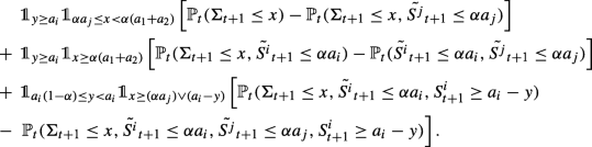
Let n ≥ 1, we are concerned with the computation of the conditional joint c.d.f. of (Γ_t+ 1,Σ_t+ 1):

In the above equation, the probability conditional on $\mathcal F_{t+\frac {1}{2}}$ can be decomposed in the following form:

$$ \begin{array}{@{}rcl@{}} &&{\mathbb P}_{t+\frac{1}{2}}\left( S_{t+1} \leq \frac{x}{n}, \tilde{S}_{t+1}\leq a_{1}\alpha,\sum\limits_{i=1}^{n}(a_{i}-S_{t+1})^{+}\leq y \right) \end{array} $$

(1.3)

$$ \begin{array}{@{}rcl@{}} &+\cdots+&{\mathbb P}_{t+\frac{1}{2}}\left( S_{t+1} \leq \frac{x}{n}, a_{j}\alpha< {\widetilde{S}}_{t+1}\leq a_{j+1}\alpha, {\sum}_{i=j+1}^{n}(a_{i}-S_{t+1})^{+}\leq y \right) \end{array} $$

(1.4)

$$ \begin{array}{@{}rcl@{}} &+\cdots+& {\mathbb P}_{t+\frac{1}{2}}\left( S_{t+1} \leq \frac{x}{n}, {\widetilde{S}}_{t+1}\geq a_{n}\alpha \right). \end{array} $$

(1.5)

It is easily seen that the term (1.3) can be written as

${\mathbb P}_{t+\frac {1}{2}}\left ({\widetilde {S}}_{t+1}\leq a_{1}\alpha , \frac {1}{n}({\sum }_{i=1}^{n}a_{i}-y)\leq S_{t+1}\leq \frac {x}{n}\wedge a_{1}\alpha \right ),$

and similarly the term (1.4) as

${\mathbb P}_{t+\frac {1}{2}}\left (a_{j}\alpha < {\widetilde {S}}_{t+1}\leq a_{j+1}\alpha , \frac {1}{n-j}({\sum }_{i=j+1}^{n}a_{i}-y)\leq S_{t+1}\leq \frac {x}{n}\wedge a_{j+1}\alpha \right ).$

Moreover, we use Markov property and Proposition 6 to write the term (1.5) in the following form

On $\{\frac {1}{n}({\sum }_{i=1}^{n}a_{i}-y)\leq \frac {x}{n}\wedge a_{1}\alpha \}$, the term (1.3) is equal to:

On $\{\frac {1}{n-j}({\sum }_{i=1+j}^{n}a_{i}-y)\leq \frac {x}{n}\wedge a_{j+1}\alpha \}$ the term (1.4) is equal to:

We conclude the proof using Theorem A.1 to compute the expectations conditional to ${\mathcal {F}}_{t}$.

B Correlated securities

In order to prove our results in the correlated case, we shall need the joint distribution of two correlated Brownian motions with drift and their suprema. The joint distribution is obtained by making the following change of variables x₂ = M₂ − σ₂r sin 𝜃 and $x_{1}=M_{1}-\sigma _{1}r(\rho \sin \theta +\sqrt {1-\rho ^{2}}\cos \theta )$ in Lemma 3 and Remark 4 from He et al. (1998).

Proposition 8

Let $X^{i}=\mu _{i}t+\sigma _{i}{W^{i}_{t}}$, where $\mu _{i}\in {\mathbb {R}}$, σ_i > 0 and Wⁱ two correlated Brownian motions with correlation coefficient ρ ∈] − 1, 1[. For x₁ ≤ M₁, x₂ ≤ M₂ with M₁, M₂ ≥ 0, we have :

${\mathbb P}({X^{1}_{t}}\in dx_{1}, {X^{2}_{t}}\in dx_{2}, sup_{u\leq t}{X^{1}_{u}}\leq M_{1} , sup_{u\leq t}{X^{2}_{u}}\leq M_{2})=p(r,r_{0}, \theta , \theta _{0}, t ; M_{1},M_{2})drd\theta$

${\mathbb P}(\tilde {X^{1}}_{0\rightarrow t}\leq M_{1} , \tilde {X^{2}}_{0\rightarrow t}\leq M_{2})=q(r_{0}, \theta _{0}, t ; M_{1}, M_{2})$, wherep andq are given in Definition 4.1 and

$$ \begin{array}{@{}rcl@{}} r&=&\frac{1}{\sqrt{1-\rho^{2}}}\sqrt{\frac{(M_{1}-x_{1})^{2}}{{\sigma_{1}^{2}}}-2\rho\frac{(M_{1}-x_{1})(M_{2}-x_{2})}{\sigma_{1}\sigma_{2}}+\frac{(M_{2}-x_{2})^{2}}{{\sigma_{2}^{2}}}},\\ r_{0}&=&\frac{1}{\sqrt{1-\rho^{2}}}\sqrt{\frac{{M_{1}^{2}}}{{\sigma_{1}^{2}}}-2\rho\frac{M_{1}M_{2}}{\sigma_{1}\sigma_{2}}+\frac{{M_{2}^{2}}}{{\sigma_{2}^{2}}}}, \tan\beta=-\frac{\sqrt{1-\rho^{2}}}{\rho}, \beta\in[0, \pi],\\ \tan\theta&=&\sqrt{1-\rho^{2}}\left( \frac{\sigma_{2}(M_{1} - x_{1})}{\sigma_{1}(M_{2} - x_{2})} - \rho\right)^{-1}, \tan \theta_{0} = \sqrt{1 - \rho^{2}}\left( \frac{\sigma_{2}M_{1}}{\sigma_{1}M_{2}} - \rho\right)^{-1}, \theta,\theta_{0}\!\in\![0, \beta]. \end{array} $$

For some special correlation values, the function q may be written in a simpler form (see Corollary 2 in He et al. 1998). We easily obtain the following results¹ :

Lemma B.1

Under the assumptions of Proposition 8, if$\rho _{n}=-\cos \frac {\pi }{n}$, we have :

$$ \begin{array}{@{}rcl@{}} \text{where }\ p(x_{1},x_{2}, t ; M_{1},M_{2})&=&e^{\alpha_{1}x_{1}+\alpha_{2}x_{2}+bt}\sum\limits_{k=1}^{n-1}\left[g_{k}^{+}(x_{1},x_{2},t)+ g_{k}^{-}(x_{1},x_{2},t) \right],\\ q(M_{1}, M_{2}, t)&=&\sum\limits_{k=0}^{n-1}\left[ Q^{+}(M_{1}, M_{2}, \frac{2k\pi}{n}+\theta)- Q^{-}(M_{1}, M_{2}, \frac{2k\pi}{n}-\theta)\right], \end{array} $$

$$ \begin{array}{@{}rcl@{}} &&g_{k}^{^{+}_{-}}(x_{1},x_{2},t)=^{+}_{-}\frac{1}{2\pi t}\exp\left\{- \frac{1}{2t}\left[ \left( \frac{1}{\sqrt{1-{\rho_{n}^{2}}}}\left( \frac{M_{1}-x_{1}}{\sigma_{1}}-\rho_{n}\frac{M_{2}-x_{2}}{\sigma_{2}}\right)+\xi_{1}\right)^{2}\right.\right.\\ &&\left.\left.+ \left( \frac{M_{2}-x_{2}}{\sigma_{2}}-\xi_{2}\right)^{2} \right] \right\},\\ &&Q^{^{+}_{-}}(M_{1}, M_{2}, \frac{2k\pi}{n} {^{+}_{-}}\theta)=\exp\left[B_{0}+B_{1}\xi_{1}+B_{2}\xi_{2}+(\frac{{B_{1}^{2}}+{B_{2}^{2}}}{2}+b)t\right]\times\\ && \qquad\qquad\qquad\quad\qquad\qquad \times {\Phi}\left( \frac{\xi_{2}+B_{2}t}{\sqrt{t}}, \frac{-\sqrt{1 - {\rho_{n}^{2}}}(\xi_{1} + B_{1}t)+\rho_{n}(\xi_{2}+B_{2}t)}{\sqrt{t}}, \rho_{n}\right),\\ && \xi_{1}=-r_{0}\cos\left( \frac{2k\pi}{n} {^{+}_{-}}\theta\right), \xi_{2}=r_{0}\sin\left( \frac{2k\pi}{n}{^{+}_{-}}\theta\right),\\ && \tan\theta=-\frac{\sqrt{1-{\rho_{n}^{2}}}}{\rho_{n}-\frac{M_{1}\sigma_{2}}{M_{2}\sigma_{1}}}, r_{0}=\frac{1}{\sqrt{1-{\rho_{n}^{2}}}}\sqrt{\frac{{M_{1}^{2}}}{{\sigma_{1}^{2}}}-2\rho_{n}\frac{M_{1}M_{2}}{\sigma_{1}\sigma_{2}}+\frac{{M_{2}^{2}}}{{\sigma_{2}^{2}}}},\\ && B_{0}=a_{1}M_{1}+a_{2}M_{2}, B_{1}=a_{1}\sigma_{1}\sqrt{1-{\rho_{n}^{2}}}, B_{2}=-(a_{1}\sigma_{1}\rho_{n}+a_{2}\sigma_{2})=\frac{-\alpha_{2}}{\sigma_{2}},\\ && b=-\frac{{\alpha_{1}^{2}}{\sigma_{2}^{2}}+{\alpha_{2}^{2}}{\sigma_{1}^{2}}}{2(1-{\rho_{n}^{2}}){\sigma_{1}^{2}}{\sigma_{2}^{2}}}+\frac{\rho_{n}\alpha_{1}\alpha_{2}}{(1-{\rho_{n}^{2}})\sigma_{1}\sigma_{2}}, a_{1}=\frac{\alpha_{1}\sigma_{2}-\rho_{n}\alpha_{2}\sigma_{1}}{(1-{\rho_{n}^{2}}){\sigma_{1}^{2}}\sigma_{2}}, a_{2}=\frac{\alpha_{2}\sigma_{1}-\rho_{n}\alpha_{1}\sigma_{2}}{(1-{\rho_{n}^{2}})\sigma_{1}{\sigma_{2}^{2}}}. \end{array} $$

2.1 B.1 Proof of Proposition 5

We remark that

$$ \begin{array}{@{}rcl@{}} {\mathbb P}_{s}({\Gamma}_{t}>0)&=&1-{\mathbb P}_{s}({\Gamma}_{t}=0)={\mathbb P}_{s}\left( \tilde{S}^{1}_{t}\leq\alpha a_{1}\right)+{\mathbb P}_{s}\left( \tilde{S}^{2}_{t}\leq\alpha a_{2}\right)\\ &&-\mathbb{P}_{s}\left( \tilde{S}^{1}_{t}\leq\alpha a_{1}, \tilde{S}^{2}_{t}\leq\alpha a_{2}\right)\\ &=&\sum\limits_{i=1}^{2}p_{i}(a_{i}, {S^{i}_{s}})-{\mathbb P}_{s}\left( {\mathbb P}_{t-1/2}\left( \tilde{S}^{1}_{t}\leq\alpha a_{1}, \tilde{S}^{2}_{t}\leq\alpha a_{2}\right)\right). \end{array} $$

Markov property, Proposition 8 and writing $S^{1}_{t-1/2}={S^{1}_{s}}e^{\mu _{1}(\delta -1/2)+\sigma _{1}\sqrt {\delta -1/2}X}$ with $X\sim {\mathcal {N}}(0,1)$ lead to the desired formula.

We need some technical results in order to find the joint law of Γ and Σ.

Lemma B.2

Letx > 0. The c.d.f of the aggregate dynamics Σ of two correlated shares is given by

where X is a standard Gaussian r.v. We denote this probability by $f({S^{1}_{t}}, {S^{2}_{t}}, x)=\mathbb {P}_{t}({\Sigma }_{t+1}\geq 0).$

Proof

Since W¹ and W² are two correlated Brownian motions with correlation coefficient ρ, then $W^{2}=\rho W^{1} +\sqrt {1-\rho ^{2}}W$ with W¹ and W two independent BM. Hence :

$$ {\mathbb P}_{t}({\Sigma}_{t+1}\leq 0)={\mathbb P}_{t}({S^{1}_{t}}e^{\mu_{1}+\sigma_{1}X}+{S^{2}_{t}}e^{\mu_{2}+\sigma_{2}\rho X+\sigma_{2}\sqrt{1-\rho^{2}}Z}\leq x), $$

where X and Z are two independent standard Gaussian r.v. We integrate with respect Z and the conclusion holds. □

Lemma B.3

Let${X^{i}_{t}}=\mu _{i}t+\sigma _{i}{W^{i}_{t}}$, where$\mu _{i}, \sigma _{i}\in {\mathbb {R}}$andWⁱtwo correlated BM withcorrelation coefficientρ ∈] − 1, 1[. Then forM₁ > 0, $x_{1}, x_{2}\in \mathcal {R}$

$${\mathbb P}({X^{1}_{t}}\in dx_{1}, {X^{2}_{t}}\in dx_{2}, sup_{u\leq t}{X^{1}_{u}}\leq M_{1})=h(x_{1},x_{2},M_{1})dx_{1}dx_{2}$$

where

Proof

Without loss of generality we consider σ_i = 1, i = 1, 2 (we then replace x₁, M₁, x₂ by $\frac {x_{1}}{\sigma _{1}}, \frac {M_{1}}{\sigma _{1}}, \frac {x_{2}}{\sigma _{2}}$). Since

$$\mathbb{P}({X^{1}_{t}}\in dx_{1}, {X^{2}_{t}}\in dx_{2}, sup_{u\leq t}{X^{1}_{u}}\leq M_{1})=\frac{\partial^{2}}{\partial x_{1} \partial x_{2}}\mathbb{P}({X^{1}_{t}}\leq x_{1}, {X^{2}_{t}}\leq x_{2}, sup_{u\leq t}{X^{1}_{u}}\leq M_{1})$$

and $W^{2}=\rho W^{1} +\sqrt {1-\rho ^{2}}W$ with W¹ and W two independent BM, we can write for ρ≠ 0²

The derivative of the first term is 0. For the second term, we integrate with respect to the law of W_t and then we use Proposition 6. Finally the derivative with respect to x₁ and x₂ leads to the desired result. □

We easily deduce the following :

Corollary B.3.1

Under the assumptions of Lemma B.3 letR₁, R₂, x, w, M₁ > 0. Then

where X is a standard Gaussian r.v.

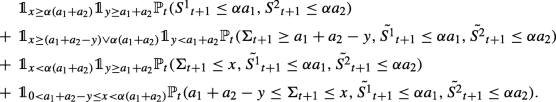
2.2 B.2 Proof of Proposition 4.2

The joint c.d.f

can be decomposed in the following form :

$$ \begin{array}{@{}rcl@{}} &&{\mathbb P}_{t}\left( S^{1}_{t+1} +S^{2}_{t+1}\leq x, \tilde{S^{1}}_{t+1}>\alpha a_{1}, \tilde{S^{2}}_{t+1}>\alpha a_{2} \right)\\ &+&\sum\limits_{i,j\in\{1,2\}, i\neq j}{\mathbb P}_{t}\left( S^{1}_{t+1} +S^{2}_{t+1}\leq x, \tilde{S^{i}}_{t+1}\leq\alpha a_{i}, \tilde{S^{j}}_{t+1}>\alpha a_{j}, S^{i}_{t+1}\geq a_{i}-y \right)\\ &+& {\mathbb P}_{t}\left( a_{1}+a_{2}-y\leq S^{1}_{t+1} +S^{2}_{t+1}\leq x, \tilde{S^{1}}_{t+1}\leq\alpha a_{1}, \tilde{S^{2}}_{t+1}\leq\alpha a_{2} \right). \end{array} $$

Step 1 - Probabilities decomposition :

• The first term $C_{1}({S^{1}_{t}}, {S^{2}_{t}})={\mathbb P}_{t}\left (S^{1}_{t+1} +S^{2}_{t+1}\leq x, \tilde {S^{1}}_{t+1}>\alpha a_{1}, \tilde {S^{2}}_{t+1}>\alpha a_{2} \right )$ may be written as :

Recall that $S^{1}_{t+1} +S^{2}_{t+1}={\Sigma }_{t+1}$. Note that on {x ≥ α(a₁ + a₂)},

$${\mathbb P}_{t}\left( S^{1}_{t+1} +S^{2}_{t+1}\leq x, \tilde{S^{1}}_{ t+1}\leq\alpha a_{1}, \tilde{S^{2}}_{t+1}\leq\alpha a_{2} \right)=\mathbb{P}_{t}\left( \tilde{S^{1}}_{t+1}\leq\alpha a_{1}, \tilde{S^{2}}_{t+1}\leq\alpha a_{2} \right).$$

Hence,

• The second term $C_{2}({S^{i}_{t}}, {S^{j}_{t}}, a_{i},a_{j})={\mathbb P}_{t}\left (S^{1}_{t+1} +S^{2}_{t+1}\leq x, \tilde {S^{i}}_{t+1}\!\leq \!\alpha a_{i}, \tilde {S^{j}}_{t+1}\!>\!\alpha a_{j}, S^{i}_{t+1}\geq a_{i}-y \right )$ equals to :

• The last term $C_{3}({S^{1}_{t}}, {S^{2}_{t}})={\mathbb P}_{t}\left (a_{1}+a_{2}-y\leq S^{1}_{t+1} +S^{2}_{t+1}\leq x, \tilde {S^{1}}_{t+1}\leq \alpha a_{1}, \tilde {S^{2}}_{ t+1} \leq \alpha a_{2} \right )$ may be written as :

Step 2 - Grouping of terms :

Remark that for the term $C_{2}({S^{i}_{t}}, {S^{j}_{t}}, a_{i},a_{j})$, we may use Markov property and Proposition 8. Hence we can write (consider for example the case i = 1 and j = 2) :

where ${X^{i}_{t}}=\mu _{i}t+\sigma _{i}{B^{i}_{t}}$ where Bⁱ are two correlated BM independent of $\mathcal {F}_{t+\frac {1}{2}}$, and D₁ given before.

The same reasoning allows to write ${\mathbb P}_{t}({\Sigma }_{t+1}\leq x, \tilde {S^{1}}_{t+1}\leq \alpha a_{1}, \tilde {S^{2}}_{t+1}\leq \alpha a_{2}, S^{2}_{t+1}\geq a_{2}-y)$, ${\mathbb P}_{t}({\Sigma }_{t+1}\geq a_{1}+a_{2}-y, \tilde {S^{1}}_{t+1}\leq \alpha a_{1}, \tilde {S^{2}}_{t+1}\leq \alpha a_{2})$, $\mathbb {P}_{t}({\Sigma }_{t+1}\leq x, \tilde {S^{1}}_{ t+1}\leq \alpha a_{1}, \tilde {S^{2}}_{t+1}\leq \alpha a_{2})$ and $\mathbb {P}_{t}(a_{1}+a_{2}-y\leq {\Sigma }_{t+1}\leq x, \tilde {S^{1}}_{t+1}\leq \alpha a_{1}, \tilde {S^{2}}_{t+1}\leq \alpha a_{2})$ in a similar form with D₂, D₃(a₁ + a₂ − y), D₃(x) and D₃(x) − D₃(a₁ + a₂ − y).

Hence, we have

Step 3 - Final calculation :

Remark that ${\mathbb P}_{t}(\tilde {S^{1}}_{t+1}\leq \alpha a_{1}, \tilde {S^{2}}_{t+1}\leq \alpha a_{2})=Q({S^{1}_{t}}, {S^{2}_{t}}, 1)$ with Q given in Proposition 5. Also, the conditional law of Σ, i.e. $\mathbb {P}_{t}({\Sigma }_{t+1}\leq x)$, is given in Theorem B.2. Since the calculation method is the same for all the other terms, we only detail here the probability $\mathbb {P}_{t}({\Sigma }_{t+1}\leq x, \tilde {S^{1}}_{t+1}<\alpha a_{1})$. Thus, Markov property gives

where $X^{i}_{\frac {1}{2}}=\frac {\mu _{i}}{2}+\sigma _{i}B^{i}_{\frac {1}{2}}$, Bⁱ two correlated BM independent of $\mathcal {F}_{t+\frac {1}{2}}$. Next, using Corollary B.3.1, we find that $\mathbb {P}_{t+\frac {1}{2}}\left (S^{1}_{t+\frac {1}{2}} e^{X^{1}_{\frac {1}{2}}}+S^{2}_{t+\frac {1}{2}} e^{X^{2}_{\frac {1}{2}}}\leq x, \tilde {X}^{1}_{ \frac {1}{2}}<\ln \frac {\alpha a_{1}}{S^{1}_{t+\frac {1}{2}}} \right )$ equals

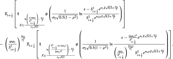
where Z is a standard Gaussian r.v. independent of $\mathcal {F}_{t+\frac {1}{2}}$.

We conclude writing $S^{1}_{t+\frac {1}{2}}={S^{1}_{t}}+\frac {\mu _{1}}{2}+\sigma _{1}\sqrt {0.5}X$ (resp. $S^{2}_{t+\frac {1}{2}}={S^{2}_{t}}+\frac {\mu _{2}}{2}+\sigma _{2}\sqrt {0.5}Y$) with X, Y two correlated standard Gaussian r.v’s, that:

We also find

Remark that on I₁, x > αa₁, so :

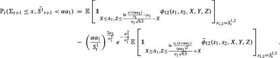
$$ \begin{array}{@{}rcl@{}} &&{\mathbb P}_{t}({\Sigma}_{t+1}\leq x, \tilde{S^{1}}_{t+1}<\alpha a_{1})+ {\mathbb P}_{t}({\Sigma}_{t+1}\leq x, \tilde{S^{1}}_{t+1}\leq\alpha a_{i}, S^{1}_{t+1}\geq a_{1}-y)\\ &&= {\mathbb{E}}\left[ J_{1}(s_{1},s_{2},X,Z)\phi_{12}(s_{1}, s_{2},X,Y,Z)\right]\\ &&\quad-\left( \frac{\alpha a_{1}}{{S^{1}_{t}}}\right)^{\frac{2\mu_{1}}{{\sigma^{2}_{1}}}}e^{-\frac{{\mu^{2}_{1}}}{{\sigma^{2}_{1}}}}\mathcal{E}\left[ J_{2}(s_{1},s_{2},X,Z)\tilde{\phi}_{12}(s_{1}, s_{2},X,Y,Z)\right]. \end{array} $$

This completes the proof.

C Additional Figures

Fig. 4

Joint distribution function. The joint probability $\mathbb P_{t}({\Gamma }_{t+1}<y, {\Sigma }_{t+1}\leq x )$ in Proposition 4.1 (left) and Proposition 4.2 (right), for t = 0 with n = 2. The input parameters are as follows α = 80%, r = 1%. Comonotonic shares: acquisition values $S^{1}_{t_{1}}=80$ and $S^{1}_{t_{2}}=90$ and initial value ${S^{1}_{0}}=120$

Fig. 5

Joint distribution function. The joint probability $\mathbb P_{t}({\Gamma }_{t+1}<y, {\Sigma }_{t+1}\leq x)$ in Proposition 4.1, for t = 0, with acquisition values a₁ = 80 and a₂ = 90 and initial value S₀ = 120 (left) and S₀ = 60 (right)

References

Azzaz J, Loisel S, Thérond P-E (2015) Some characteristics of an equity security next-year impairment. Rev Quant Finan Acc 45(1):111–135
Bennemann C, Hennig C (2010) Impairment estimates of equity portfolios represented by model points. Belgian Act Bullet 9(1):43–49
Black F, Scholes M (1973) The pricing of options and corporate liabilities. J Polit Econ 81(3):637–654
Escobar M, Hernandez J (2014) A note on the distribution of multivariate brownian extrema. International Journal of Stochastic Analysis
Gobet E (2000) Weak approximation of killed diffusion using euler schemes. Stoch Process Appl 87(2):167–197
Harrison MJ (1985) Brownian Motion and Stochastic Flow Systems. Wiley, New York
He H, Keirstead W, Rebholz J (1998) Double lookbacks. Math Financ 8 (3):201–228
Keller JB (1953) The scope of the image method. Commun Pure Appl Math 6 (4):505–512
Thérond P-E (2016) About Market Consistent Valuation in Insurance. In: Laurent J-P, Norberg R, Planchet F (eds) Modelling in Life Insurance: A Management Perspective, chapter 2. Springer, pp 43–60
Vedani J, El Karoui N, Loisel S, Prigent JL (2017) Market inconsistencies of market-consistent European life insurance economic valuations: pitfalls and practical solutions. European Actuarial Journal 7(1)
Wüthrich M (2016) Market-Consistent Actuarial Valuation. Springer, Berlin
Author information
Authors and Affiliations
Corresponding author
Additional information
Publisher’s Note
Springer Nature remains neutral with regard to jurisdictional claims in published maps and institutional affiliations.
This work has been supported by the BNP Paribas Cardif Chair ”Data Analitycs and Models in Insurance”. The views expressed in this document are the authors owns and do not necessarily reflect those endorsed by BNP Paribas Cardif.