Grid design and numerical modeling of multiphase flow in complex reservoirs using orthogonal collocation schemes

Abstract

An advanced grid system design was developed to capture accurately the effects of geometrically complex features such as geological features (faults, pinch outs and inclined beddings) and well-related phenomenon (multilateral wells of general orientation) in triangular coordinates. Modeling these effects can have significant impact on the accuracy of the simulation and prediction of reservoir performance as well as reservoir fluid flow using conventional grid designs. The finite difference method provides additional difficulty in capturing geological features in typical reservoir flow and grid model simulators. Hence, the orthogonal collocation method was used for simulating multiphase reservoir flow equations in triangular curvilinear coordinates $\left[ {\xi \left( r \right),\xi \left( \theta \right),\xi \left( z \right)} \right]$ of domain [0,1] that were derived from Cartesian coordinates $\left( {x,y,z} \right)$. This was to accommodate general three-dimensional deviated wells and complex reservoir geometry for multiphase flow of hydrocarbon in complex reservoir formations. Based on preliminary field data obtained from multinational oil and gas operator in Nigeria, the proposed model was used to predict saturation, production and petroleum productivity with time and distance in a MATLAB environment. The simulated plots revealed that pressure is parabolic at the center of the reservoir with coordinates $\xi (r) =0.4257$, reflecting the impact of geological features in the pressure and production flow performance.

Introduction

Several approaches for modeling geometrically complex features have been documented in the literature. Azim and Abdelmoneim [1] presented mathematical model to describe the flow of reservoir fluid in hydraulically fractured reservoir using finite difference simulators in a manner that would allow the simulator to mimic the actual fracture geometry without dramatically increasing the number of grid cells and hence increasing the computing requirements and time. Their proposed design was applied to an anonymous field in the western dessert in Egypt and their simulated results were compared with the actual production data which was recorded after the fracture to verify that the model was capable of modeling the actual reservoir performance. Jacquemyn et al. [2] presented an approach that used a grid-free non-uniform rational B-splines (NURBS) curves and surfaces to represent realistic surface-based geological reservoir modeling that was based on a boundary representation in which all heterogeneity of interest (structural, stratigraphic, sedimentological, diagenetic) was modeled by its bounding surfaces, independent of any grid. However, the most general approaches for modeling geometrically complex features involve the use of fully unstructured grids (triangular grids in two dimensions and tetrahedral or prismatic grids in three dimensions) or structured grids coupled with locally unstructured grids. In addition, several technical issues must be resolved before highly complex geometrical features can be gridded and modeled in practice [3,4,5]. Modular gridding makes use of different grid types in different regions of the reservoir. For example, around a deviated or horizontal well, the grid might be radial (or nearly so); while in the vicinity of a complex multilateral well, the grid could be fully unstructured. Examples of fully unstructured grid systems include grids based on tetrahedral, pyramid, or prismatic elements. Previous techniques usually require highly robust unstructured gridding procedures. Jenny et al. [6, 7] provided an alternate approach to the modeling of geometrically complex features by hexahedral multi-block grids. These grids are locally structured (meaning they possess a logical $i,\,j,\,k$ ordering locally) but are globally unstructured. Thus, they are adept at capturing many types of features, such as faults (the local grid is oriented with the fault) or deviated wells (the grid near the well is approximately radial).

According to Edwards [8], hexahedral multi-block grids result in locally structured linear systems, which are more computationally efficient to solve than fully unstructured systems. In addition, these approaches provide a very natural framework for parallel computation. The hexahedral multi-block methods were developed and applied previously within a finite difference context by Edwards [3] and within a mixed finite element context by Arbogast et al. [4] and Wheeler et al. [5]. Edwards [1] used a multi-block approach to model two-dimensional sand/shale systems.

According to Castellini et al. [9], Edwards [10, 11], Edwards and Rogers [12], and Portella and Hewett [13], development of grid generation techniques and numerical methods that can reliably compute the physically correct solution to complex simulation problems on three-dimensional flexible grids are understudied. Structured and unstructured grid generation techniques are currently being developed. The need for unstructured grids can arise locally when modeling complex deviated wells, faults, pinch outs or when increasing local grid resolution (local grid refinement). For complex reservoir boundaries, the task of generating a grid can sometimes be simplified by employing direct triangulation. To allow general flexibility, a multiblock method is being developed, where the reservoir domain can be decomposed into a structured or unstructured set of sub-domains where each sub-domain grid is structured (logically Cartesian). Future work will include the development of interfaces that will allow a discontinuous change in logical coordinate density so that locally unstructured grids can be used for specific regions or sub-domains of the reservoir.

Flow simulations of reservoir systems with complex geometries and geological features generally require the use of flexible structured and unstructured grids to resolve important features such as faults and deviated wells [14, 15]. Corner-point geometry (or non-orthogonal grids) is widely used in reservoir simulation. These grids are structured (logically Cartesian) and are comprised of quadrilateral cells. Unstructured grids are generally comprised of triangular, and/or quadrilateral cells (in 2D) and are generally based on a more complex data structure than the standard logically Cartesian grid indices. Several Grid Design types have been reported in the literature [16, 17].

The generation of a grid via a single technique such as an algebraic method [18], Thompson mapping [19], conformal mapping or even streamlines and equipotentials though may prove to be adequate for certain reservoir types, inherent complexity of reservoir systems resulting from existence of geological features such as, pinch out, well deviated, faults may lead to generation of problem of specific grids that allow the prediction of accurate pressure and saturation profiles.

A recent advancement on a grid methodology is now reported. The significant errors inherent in existing approaches and the improved results that are possible have led to the development of a new numerical grid methodology for simulating complex and non-complex reservoir systems. The technique transforms the unstructured Cartesian coordinates $\left( {x,\,\,y,\,\,z} \right)$ of the reservoir into a locally structured dimensionless curvilinear coordinates $\left[ {\xi \left( r \right),\xi \left( \theta \right),\xi \left( z \right)} \right]$ using a transformation triangular coordinates system that renders the grid systems dimensionless to unity in domain [0,1]. The transformed flow reservoir model was numerically solved using orthogonal collocation method. The re-transformation to the original plane in Cartesian coordinates also uses an inverse transformation model. The inaccuracy and difficulty in modeling and simulating multiphase flow of complex reservoirs has been significantly reduced through the use of a transformed reservoir model, which was solved in the triangular curvilinear dimensionless plane that can only have spatial coordinates [0,1]. The unique attribute of the proposed model in this study is that it uses the ten collocation grid points to transform into triangular coordinates instead of multiblocks cells. This has significantly reduced the complexity of the various attributes of the reservoir into a simple grid collocation points with coordinates in triangular plane that cannot exceed one or be less than zero.

Construction of the reservoir grid

The approach presented in this study requires the construction of the reservoir grid from a set of collocation grid points, where each local collocation grid point is appropriately chosen according to the local geometry, geology and/or mean (representative) flow conditions. Accordingly, the reservoir is decomposed into a set of sub-domains of collocation points in the overall grid design architectures linked by the hexahedral block.

It is important to note that there are several grid design types based on modular discretization schemes that have been reported. Extensive literature on the subject matter of grid designs and methodology abounds, which may interest prospective readers of this paper. However, some current grid designs and models reported in literature are presented, thus:

• 1. Algebraic grid generation The default grid is defined by the transfinite interpolant method.

• 2. Elliptic grid generation Here, it is used to denote a class of grid generation techniques that involve solving a coupled set of elliptic partial differential equations to generate grid coordinates.

• 3. Flow-based grid generation It is used here to denote grids that are generated by using streamline or flow field information to determine local grid node density and coordinate line orientation.

When heterogeneity is present, key requirements of an optimal subdomain module are that the grid be dense in high flow regions so as to resolve connected flow paths of the reservoir or subdomain.

Previous approach in modular reservoir gridding

The previous approach in modular reservoir gridding includes the Finite Volume Scheme in which the most common reservoir simulation schemes are cell (block) centered or point distributed where flow variables and rock properties are assumed to have piecewise constant variations with respect to the control volumes of the mesh. The permeability tensor is assumed to be diagonal and control-volume face fluxes are proportional to the harmonic mean of adjacent cell permeabilities multiplying their corresponding discrete pressure differences; e.g., at face $\left( {i\, + \,{\raise0.7ex\hbox{$1$} \!\mathord{\left/ {\vphantom {1 2}}\right.\kern-0pt} \!\lower0.7ex\hbox{$2$}},\,\,j,\,\,k} \right)$, the flux takes the well-known form of Eq. (1):

$$F_{i + 1/2,j,k} \left( \phi \right) = - \frac{{2\left( {K_{11} } \right)_{i,j,k} \left( {K_{11} } \right)_{i + 1,j,k} \Delta y}}{{\left[ {\left( {K_{11} } \right)_{i,j,k} + \left( {K_{11} } \right)_{i + 1,j,k} } \right]\Delta x}}\left( {\phi_{i + 1,j,k} - \phi_{i,j,k} } \right)$$

(1)

Developments in reservoir multiphase flow modeling and simulation

Without loss of generality, the schemes presented here are illustrated with respect to two-phase flow models, with unit porosity and with capillary pressure neglected. The continuity equation for each phase $j$ is written as, thus:

$$\oint_{\varOmega } {\left[ {\left( {\frac{{\partial s_{p} }}{\partial t}} \right) + \nabla \cdot v_{p} } \right]\text{d}\tau = m_{p} \left( {x,y} \right)}$$

(2)

This approximation gives rise to a five-point scheme in two dimensions and a seven-point scheme in three dimensions. In this work, a fully implicit formulation [20] was used to solve Eq. (2) and was written in the locally conservative integral form thus:

$$\left( {s_{pi,j,k}^{n+1} - s_{pi,j,k}^{n} } \right)\tau_{i,j,k} + \Delta t\left[ \begin{aligned} \lambda_{p} \left( {s_{pi + 1/2,j,k}^{n+1} } \right)F_{i + 1/2,j,k} \left( {\phi^{n + 1} } \right) - \lambda_{P} \left( {s_{pi - 1/2,j,k}^{n+1} } \right)F_{i - 1/2,j,k} \left( {\phi^{n + 1} } \right) \hfill \\ + \lambda_{p} \left( {s_{pi,j + 1/2,k}^{n+1} } \right)F_{i,j + 1/2,k} \left( {\phi^{n + 1} } \right) - \lambda_{P} \left( {s_{pi,j - 1/2,k}^{n+1} } \right)F_{i,j - 1/2,k} \left( {\phi^{n + 1} } \right) \hfill \\ + \lambda_{p} \left( {s_{pi,j,k + 1/2}^{n+1} } \right)F_{i,j,k + 1/2} \left( {\phi^{n + 1} } \right) - \lambda_{P} \left( {s_{pi,j,k - 1/2}^{n+1} } \right)F_{i,j,k - 1/2} \left( {\phi^{n + 1} } \right) \hfill \\ \end{aligned} \right]=\Delta tM_{{P_{i,j,k} }}$$

(3)

For a logically Cartesian grid where $\tau_{i}$ is the control volume, the system was solved with respect to the aqueous phase saturation and pressure $\left( {s_{1} ,\varphi } \right)$; the oleic phase saturation,$s_{2}$ was deduced from Eq. (2). The hyperbolic flux contribution is up-winded according to the wave direction across each edge; e.g., at edge $\left( {i\, + \,{\raise0.7ex\hbox{$1$} \!\mathord{\left/ {\vphantom {1 2}}\right.\kern-0pt} \!\lower0.7ex\hbox{$2$}},\,\,j,\,\,k} \right)$, the direction is a function of $\lambda_{P} \left( {s_{pi + 1/2,j,k}^{n + 1} } \right)F_{i + 1/2,j,k} \left( {\phi^{n + 1} } \right)$ and for a positive outward $s_{pi + 1/2,j,k}^{n + 1} = s_{pi,j,k}^{n + 1}$ otherwise $s_{pi + 1/2,j,k}^{n + 1} = s_{pi + 1,j,k}^{n + 1}$. This method is known as the single-point upstream weighting scheme in reservoir simulation and is a function of four points of the seven-point stencil, where the four points vary according to the local upwind direction. In this case, the net fluxes of Eq. (3) comprise cell edge-based quantities. Several new schemes have been proposed and developed for full tensor simulation in recent years, which included the works of some investigators [4, 8, 10, 12, 17, 21, 22]. These schemes all employ nine-point operators for the pressure equation on logically Cartesian grids in two dimensions. In this work, cell vertex/point-distributed schemes are considered.

According to Prevost et al. [23], reservoir simulation is the process of inferring the behavior of petroleum reservoir from the performance of a model to optimize the recovery of hydrocarbons. The five major stages to the modeling process for the multiphase flow problem, and in particular to reservoir simulation, are as follows:

• 1. A physical model is developed (the Grid and Flow Model).

• 2. A mathematical model of the physical model is obtained.

• 3. A numerical scheme for solution of the mathematical model is provided.

• 4. A computer program is developed to implement the numerical model; and

• 5. Finally, examination and validation of the first four steps based on the results from the computer model.

The streamline method is based on solving the pressure field as well as the saturation distribution model [24]. One advantage of a conventional Implicit in Pressure, Explicit in Saturation, IMPES, method over the fully implicit model is that numerical error due to discretization is reduced. The trade-off is that smaller time step sizes must be taken due to stability considerations. The governing equation for flow of a component $i$ with $n_{\text{p}}$ phases in porous medium was presented by Lake [15].

The governing saturation equation for the IMPES method can be derived from Lake Equation. To simplify the problem, it is assumed that the phases are immiscible. This results in a simplified equation, thus:

$$\phi \frac{{\partial S_{j} }}{\partial t} + \nabla \cdot u_{j} = q_{\rm s} f_{j,s}$$

(4)

where ϕ is assumed constant and $f_{j,\,s}$ is the fraction contributed by phase j to $q_{s}$. Equation (4) can be expanded to incorporate the Darcy model thus:

$$\phi \frac{{\partial S_{j} }}{\partial t} + \nabla \cdot \left[ {\frac{{k_{rj} u_{t} }}{{\mu_{j} \lambda_{t} }} - \tilde{K} \cdot g\frac{{k_{rj} }}{{u_{j} \lambda_{t} }}\sum\limits_{m = 1}^{{n_{\rm p} }} {\frac{{k_{rm} }}{{\mu_{m} \left( {\rho_{m} - \rho_{j} } \right)}}} } \right] = q_{s} f_{j,s}$$

(5)

The standard Buckley–Leverett, $f_{j}$, and gravitational fractional flow term, $\tilde{G}_{j}$, are defined by Eqs. (6), (7), respectively, thus:

$$f_{j} = \frac{{k_{rj} }}{{\mu_{j} \lambda_{t} }}$$

(6)

$$\tilde{G}_{j} = - \tilde{K} \cdot g\frac{{k_{rj} }}{{\mu_{j} \lambda_{t} }}\sum\limits_{m = 1}^{{n_{p} }} {\frac{{k_{rm} }}{{\mu_{m} \left( {\rho_{m} - \rho_{j} } \right)}}}$$

(7)

Hence, Eq. (5) can be simplified to give a final saturation model, thus:

$$\phi \frac{{\partial S_{j} }}{\partial t} + \nabla \cdot \,f_{j} u_{t} + \nabla \cdot \tilde{G}_{j} = q_{s} f_{j,\,s}$$

(8)

Given that $\nabla \cdot u_{t} = 0$ for incompressible flow, the governing partial differential saturation equation of an individual phase becomes:

$$\phi \frac{{\partial S_{j} }}{\partial t} + u_{t} \cdot \nabla f_{j} +\nabla \cdot \tilde{G}_{j} = q_{s} f_{j,\,s}$$

(9)

The saturation equation is parabolic. If an oil–water system is considered and the effects of gravity and capillary pressure are neglected, the well-known pressure equation evolves.

Incorporating a geological factor $k_{gs}$ into Eq. (9) that redefines the saturation flow model, we have:

$$\phi \left( {1 + k_{gs} } \right)\frac{{\partial S_{j} }}{\partial t} + u_{t} \cdot \nabla f_{j} + \nabla \cdot \tilde{G}_{j} = q_{s} f_{j,s}$$

(10)

Reservoir flow modeling has, thus, been advanced by incorporating a complex geological factor, $k_{gs}$, in the IMPES equation. Similarly, for the pressure systems, the geological feature that transforms the pressure equation is $k_{gp}$ incorporated in the pressure model equation, which is presented, thus:

$$\phi \,c_{T} \left( {1 + k_{gp} } \right)\frac{\partial p}{\partial t} = \nabla \cdot \left[ {k\left( {\lambda_{\omega } + \lambda_{o} } \right)\nabla p} \right] + q_{w} + q_{o}$$

(11)

with $\lambda_{j} = {{k_{rj} } \mathord{\left/ {\vphantom {{k_{rj} } {\mu_{j} \quad j = o,\omega ,g}}} \right. \kern-0pt} {\mu_{j} \quad j = o,\omega ,g}}$.

There are two ways of representing fluid motion: the Eulerian and the Lagrangian. The Lagrangian representation of fluid motion includes the coordinates of the fluid’s particles $x_{i} \;\left( {i = 1,\;2,\;3} \right)$ ($x_{i}$ is used to specify the flow model in terms of time t) and some vector $\left( {\xi_{1} ,\;\xi_{2} ,\;\xi_{3} } \right)$ which identifies a given particle of the fluid. The path line is described by the solutions of three parametric equations: $x_{i} = x_{i} (\xi_{k} ,t),\;p = p(\xi_{k} ,t),\;\rho = \rho (\xi_{k} ,t),$ etc. The variables $\left( {\xi_{1} ,\;\xi_{2} ,\;\xi_{3} } \right)$ are usually assumed to be the coordinates of a fluid particle at some time $t_{0}$ (initial coordinates), i.e. $\xi_{i} = x_{i} (\xi_{k} ,t_{0} )$:

$$\left( {\frac{{\mu A_{x} {\text{d}}x}}{{K_{x} {\raise0.7ex\hbox{${\partial p}$} \!\mathord{\left/ {\vphantom {{\partial p} {\partial x}}}\right.\kern-0pt} \!\lower0.7ex\hbox{${\partial x}$}}}}} \right) = \left( {\frac{{\mu A_{y} {\text{d}}y}}{{K_{y} {\raise0.7ex\hbox{${\partial p}$} \!\mathord{\left/ {\vphantom {{\partial p} {\partial y}}}\right.\kern-0pt} \!\lower0.7ex\hbox{${\partial y}$}}}}} \right) = \left( {\frac{{\mu A_{z} {\text{d}}z}}{{K_{z} {\raise0.7ex\hbox{${\partial p}$} \!\mathord{\left/ {\vphantom {{\partial p} {\partial z}}}\right.\kern-0pt} \!\lower0.7ex\hbox{${\partial z}$}}}}} \right) = {\text{d}}t$$

(12)

For a case of an isotropic medium, $K_{x} = K_{y} = K_{z} = K$ while for an equipotential surface, p = constant. Consider elementary displacement ds in the direction normal to this surface, then $\Delta p \times {\text{d}}s = 0$, so we have:

$$\frac{{{\text{d}}x}}{{{\raise0.7ex\hbox{${\partial p}$} \!\mathord{\left/ {\vphantom {{\partial p} {\partial x}}}\right.\kern-0pt} \!\lower0.7ex\hbox{${\partial x}$}}}} = \frac{{{\text{d}}y}}{{{\raise0.7ex\hbox{${\partial p}$} \!\mathord{\left/ {\vphantom {{\partial p} {\partial y}}}\right.\kern-0pt} \!\lower0.7ex\hbox{${\partial y}$}}}} = \frac{{{\text{d}}z}}{{{\raise0.7ex\hbox{${\partial p}$} \!\mathord{\left/ {\vphantom {{\partial p} {\partial z}}}\right.\kern-0pt} \!\lower0.7ex\hbox{${\partial z}$}}}}$$

(13)

Equation (13) defines curves in space normal to the equipotential surface, which is streamline.

Development in grid system design and reservoir simulation

There are inherent errors associated with conventional grid representations, which have been addressed in this paper by the introduction of a curvilinear transformed triangular coordinate collocation point, which was solved numerically using orthogonal collocation method in a triangular curvilinear coordinate. A detailed computer flow chart that incorporates the grid design methodology is presented in Fig. 1.

Fig. 1

Flowchart for grid simulation

Grid systems design in triangular coordinates

The steps in the grid model development methodology are presented as follows:

• 1. Identify the source (injector) and sink (producer) points.

• 2. Link the collocation points with a hexahedral multi-block grid cells of the reservoir geology in Cartesian coordinates in $x,\,y,\,z$, starting from the flow source point and ending at the sink point. The source and sink represent point vertices in the hexahedral.

• 3. Transform the unstructured global Cartesian grids points $\left( {x,\,y,\,z,\,x^{\prime},\,y^{\prime},\,z^{\prime}} \right)$ hexahedral-multiple grid block into a local structured curvilinear coordinates $\left( {r,\,\theta ,\,z,\,r^{\prime},\,\theta^{\prime},\,z^{\prime}} \right)$ by a transformation such that the dimensionless spatial coordinates is within the set domain [0,1], as shown in Fig. 2.

  Fig. 2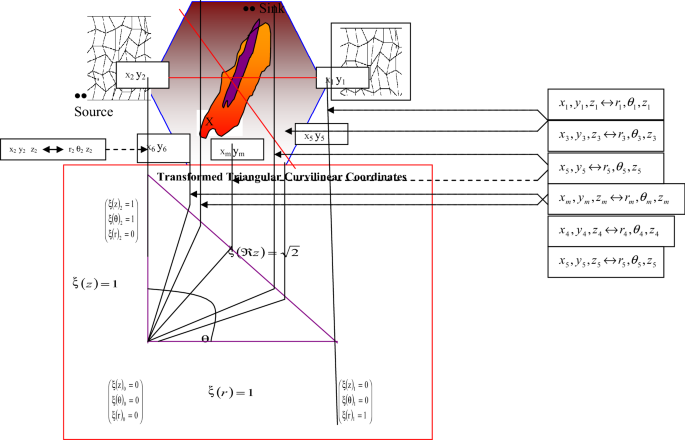

  

  Transformation of Cartesian Coordinates grid points vertices into local structured Curvilinear Coordinates

• 4. Choose a central axis and draw lines to proceed from grid points $\left( {x_{1} ,z_{1} } \right)$, $\left( {x_{2} ,z_{2} } \right)$, $\left( {x_{3} ,z_{3} } \right)$, $\left( {x_{m1} ,z_{m1} } \right)$, $\left( {x_{m2} ,z_{m2} } \right)$, $\left( {x_{4} ,z_{4} } \right)$, $\left( {x_{5} ,z_{5} } \right)$, $\left( {x_{6} ,z_{6} } \right)$ and $\left( {x^{\prime}_{1} ,z^{\prime}_{1} } \right)$, $\left( {x^{\prime}_{2} ,z^{\prime}_{2} } \right)$, $\left( {x^{\prime}_{3} ,z^{\prime}_{3} } \right)$, $\left( {x^{\prime}_{m1} ,z^{\prime}_{m1} } \right)$, $\left( {x^{\prime}_{m2} ,z^{\prime}_{m2} } \right)$$\left( {x^{\prime}_{4} ,z^{\prime}_{4} } \right)$$\left( {x^{\prime}_{5} ,z^{\prime}_{5} } \right)$ $\left( {x^{\prime}_{6} ,z^{\prime}_{6} } \right)$ in a globally unstructured Cartesian coordinates with constant width $y = d$ to meet the curvilinear triangular plane orthogonally from where they are projected to the origin to correspond to points $\left[ {\xi \left( {r_{1} } \right),\xi \left( {\theta_{1} } \right),\xi \left( {z_{1} } \right)} \right] ,$ $\left[ {\xi \left( {r_{2} } \right),\xi \left( {\theta_{2} } \right),\xi \left( {z_{2} } \right)} \right] ,$ $\left[ {\xi \left( {r_{3} } \right),\xi \left( {\theta_{3} } \right),\xi \left( {z_{3} } \right)} \right] ,$ $\left[ {\xi \left( {r_{m1} } \right),\xi \left( {\theta_{m1} } \right),\xi \left( {z_{m1} } \right)} \right],$ $\left[ {\xi \left( {r_{m2} } \right),\xi \left( {\theta_{m2} } \right),\xi \left( {z_{m2} } \right)} \right] ,$ $\left[ {\xi \left( {r_{4} } \right),\xi \left( {\theta_{4} } \right),\xi \left( {z_{4} } \right)} \right] ,$ $\left[ {\xi \left( {r_{5} } \right),\xi \left( {\theta_{5} } \right),\xi \left( {z_{5} } \right)} \right] ,$ $\left[ {\xi \left( {r_{6} } \right),\xi \left( {\theta_{6} } \right),\xi \left( {z_{6} } \right)} \right]$ and $\left[ {\xi^{\prime}\left( {r_{1} } \right),\xi^{\prime}\left( {\theta_{1} } \right),\xi^{\prime}\left( {z_{1} } \right)} \right] ,$ $\left[ {\xi^{\prime}\left( {r_{2} } \right),\xi^{\prime}\left( {\theta_{2} } \right),\xi^{\prime}\left( {z_{2} } \right)} \right] ,$ $\left[ {\xi^{\prime}\left( {r_{3} } \right),\xi^{\prime}\left( {\theta_{3} } \right),\xi^{\prime}\left( {z_{3} } \right)} \right] ,$ $\left[ {\xi^{\prime}\left( {r_{m1} } \right),\xi^{\prime}\left( {\theta_{m1} } \right),\xi^{\prime}\left( {z_{m1} } \right)} \right] ,$ $\left[ {\xi^{\prime}\left( {r_{m2} } \right),\xi^{\prime}\left( {\theta_{m2} } \right),\xi^{\prime}\left( {z_{m2} } \right)} \right] ,$ $\left[ {\xi \left( {r_{4} } \right),\xi \left( {\theta_{4} } \right),\xi \left( {z_{4} } \right)} \right] ,$ $\left[ {\xi \left( {r_{5} } \right),\xi \left( {\theta_{5} } \right),\xi \left( {z_{5} } \right)} \right] ,$ $\left[ {\xi \left( {r_{6} } \right),\xi \left( {\theta_{6} } \right),\xi \left( {z_{6} } \right)} \right]$ in a dimensionless plane, where $\xi \left( {z_{i} } \right) = \xi \left( {r_{i} } \right)\sin \left( {\xi \left( {\theta_{i} } \right)} \right)$.

• 5. Each point on the hexahedral block $\left( {x_{1} ,z_{1} } \right)$, $\left( {x_{2} ,z_{2} } \right)$, $\left( {x_{3} ,z_{3} } \right)$, $\left( {x_{m1} ,z_{m1} } \right)$,$\left( {x_{m2} ,z_{m2} } \right)$, $\left( {x_{4} ,z_{4} } \right)$, $\left( {x_{5} ,z_{5} } \right)$, $\left( {x_{6} ,z_{6} } \right)$ in the Cartesian plane represents a point for the flow or pressure variable, thus: q$\left( {x_{1} ,z_{1} } \right)$, q$\left( {x_{2} ,z_{2} } \right)$, q$\left( {x_{3} ,z_{3} } \right)$, q$\left( {x_{m1} ,z_{m1} } \right)$, q$\left( {x_{m2} ,z_{m2} } \right)$, q$\left( {x_{4} z_{4} } \right)$, q$\left( {x_{5} z_{5} } \right)$, q$\left( {x_{6} ,z_{6} } \right)$//P$\left( {x_{1} ,z_{1} } \right)$, P$\left( {x_{2} ,z_{2} } \right)$, P$\left( {x_{3} ,z_{3} } \right)$, P$\left( {x_{m1} ,z_{m1} } \right)$, P$\left( {x_{m2} ,z_{m2} } \right)$, P$\left( {x_{4} z_{4} } \right)$, P$\left( {x_{5} ,z_{5} } \right)$, P$\left( {x_{6} ,z_{6} } \right)$.

• 6. Each mirrored point $\left[ {\xi \left( {r_{1} } \right),\xi \left( {\theta_{1} } \right),\xi \left( {z_{1} } \right)} \right],$ $\left[ {\xi \left( {r_{2} } \right),\xi \left( {\theta_{2} } \right),\xi \left( {z_{2} } \right)} \right] ,$ $\left[ {\xi \left( {r_{3} } \right),\xi \left( {\theta_{3} } \right),\xi \left( {z_{3} } \right)} \right],$ $\left[ {\xi \left( {r_{m1} } \right),\xi \left( {\theta_{m1} } \right),\xi \left( {z_{m1} } \right)} \right] ,$ $\left[ {\xi \left( {r_{m2} } \right),\xi \left( {\theta_{m2} } \right),\xi \left( {z_{m2} } \right)} \right] ,$ $\left[ {\xi \left( {r_{4} } \right),\xi \left( {\theta_{4} } \right),\xi \left( {z_{4} } \right)} \right],$ $\left[ {\xi \left( {r_{5} } \right),\xi \left( {\theta_{5} } \right),\xi \left( {z_{5} } \right)} \right] ,$ $\left[ {\xi \left( {r_{6} } \right),\xi \left( {\theta_{6} } \right),\xi \left( {z_{6} } \right)} \right]$ on the transformed triangular plane represents a point mirror for the flow or pressure variable p$\left[ {\xi \left( {r_{1} } \right),\xi \left( {\theta_{1} } \right),\xi \left( {z_{1} } \right)} \right],$ p$\left[ {\xi \left( {r_{2} } \right),\xi \left( {\theta_{2} } \right),\xi \left( {z_{2} } \right)} \right],$ p$\left[ {\xi \left( {r_{3} } \right),\xi \left( {\theta_{3} } \right),\xi \left( {z_{3} } \right)} \right],$ p$\left[ {\xi \left( {r_{m1} } \right),\xi \left( {\theta_{m1} } \right),\xi \left( {z_{m1} } \right)} \right],$ p$\left[ {\xi \left( {r_{m2} } \right),\xi \left( {\theta_{m2} } \right),\xi \left( {z_{m2} } \right)} \right],$ p$\left[ {\xi \left( {r_{4} } \right),\xi \left( {\theta_{4} } \right),\xi \left( {z_{4} } \right)} \right],$ p$\left[ {\xi \left( {r_{5} } \right),\xi \left( {\theta_{5} } \right),\xi \left( {z_{5} } \right)} \right],$ p$\left[ {\xi \left( {r_{6} } \right),\xi \left( {\theta_{6} } \right),\xi \left( {z_{6} } \right)} \right]$//q$\left[ {\xi \left( {r_{1} } \right),\xi \left( {\theta_{1} } \right),\xi \left( {z_{1} } \right)} \right],$ q$\left[ {\xi \left( {r_{2} } \right),\xi \left( {\theta_{2} } \right),\xi \left( {z_{2} } \right)} \right],$ q$\left[ {\xi \left( {r_{3} } \right),\xi \left( {\theta_{3} } \right),\xi \left( {z_{3} } \right)} \right],$ q$\left[ {\xi \left( {r_{m1} } \right),\xi \left( {\theta_{m1} } \right),\xi \left( {z_{m1} } \right)} \right],$ q$\left[ {\xi \left( {r_{m2} } \right),\xi \left( {\theta_{m2} } \right),\xi \left( {z_{m2} } \right)} \right],$ q$\left[ {\xi \left( {r_{4} } \right),\xi \left( {\theta_{4} } \right),\xi \left( {z_{4} } \right)} \right],$ q$\left[ {\xi \left( {r_{5} } \right),\xi \left( {\theta_{5} } \right),\xi \left( {z_{5} } \right)} \right],$ q$\left[ {\xi \left( {r_{6} } \right),\xi \left( {\theta_{6} } \right),\xi \left( {z_{6} } \right)} \right].$

• 7. Transform the Cartesian coordinates point variables $p(x_{1} ,\,z_{1} ),\,\,p(x_{2} ,\,z_{2} )$, $p(x_{3} ,\,z_{3} )$, $p(x_{m1} ,\,z_{m1} ),\,\,p(x_{m2} ,\,z_{m2} )$, $p(x_{4} ,\,z_{4} ),\,\,p(x_{5} ,\,z_{5} )$, $p(x_{6} ,\,z_{6} )$ to the Curvilinear Triangular plane by a transformation $p(r_{1} \cos \,\theta_{1} ,\,\,r_{1} \sin \,\theta_{1} ),\,\,p ( {\text{r}}_{ 2} \cos \,\theta_{2} ,\,\,r_{2} \sin \,\theta_{2} )$, $p(r_{3} \cos \,\theta_{3} ,\,\,r_{3} \sin \,\theta_{3} )$, $p(r_{m1} \cos \,\theta_{m1} ,\,\,r_{m1} \sin \,\theta_{m1} ),\,\,p ( {\text{r}}_{m 2} \cos \,\theta_{m2} ,\,\,r_{m2} \sin \,\theta_{m2} )$, $p(r_{3} \cos \,\theta_{3} ,\,\,r_{3} \sin \,\theta_{3} )$, $p(r_{m1} \cos \,\theta_{m1} ,r_{m1} \sin \,\theta_{m1} ),\,\,p ( {\text{r}}_{m 2} \cos \,\theta_{m2} ,r_{m2} \sin \,\theta_{m2} )$, $\,p(r_{4} \cos \,\theta_{4} ,\,\,r_{4} \sin \,\theta_{4} )$, $\,p(r_{5} \cos \,\theta_{5} ,\,\,r_{5} \sin \,\theta_{5} )$, $\,p(r_{6} \cos \,\theta_{6} ,\,\,r_{6} \sin \,\theta_{6} )$, where $x_{i}$ transforms to $r_{i} \cos \,\left( {\theta_{i} } \right)$, $z_{i}$ transforms to $r_{i} \sin \,\left( {\theta_{i} } \right)$ and $y_{i}$ transforms to $d_{i}$.

• 8. Transform the saturation equations in Cartesian Coordinates of Eq. (14) to Curvilinear Coordinates thus:

$$\phi \frac{{\partial S_{j} }}{\partial t} + u_{t} \cdot \left( {\frac{{\partial f_{j} }}{\partial x} + \frac{{\partial f_{j} }}{\partial z}} \right) + \left( {\frac{\partial }{\partial x} + \frac{\partial }{\partial z}} \right) \cdot \left( {G_{xj} + G_{yj} + G_{zj} } \right) = q_{s} f_{j,s}$$

(14)

Use the transformation formula given in Eqs. (15)–(20), thus:

$$\frac{{\partial f_{j} }}{\partial x} = \frac{{\partial f_{j} }}{\partial r}\frac{\partial r}{\partial x} + \frac{{\partial f_{j} }}{\partial \theta }\frac{\partial \theta }{\partial x} + \frac{{\partial f_{j} }}{\partial z}\frac{\partial z}{\partial x} = \frac{1}{\cos \theta }\frac{{\partial f_{j} }}{\partial \xi (r)} - \frac{1}{r\sin \theta }\frac{{\partial f_{j} }}{\partial \xi (\theta )}$$

(15)

$$\frac{{\partial f_{j} }}{\partial y} = \frac{{\partial f_{j} }}{\partial r}\frac{\partial r}{\partial y} + \frac{{\partial f_{j} }}{\partial \theta }\frac{\partial \theta }{\partial y} + \frac{{\partial f_{j} }}{\partial z}\frac{\partial z}{\partial y} = \frac{1}{\sin \theta }\frac{{\partial f_{j} }}{\partial \xi (r)} + \frac{1}{r\,\cos \theta }\frac{{\partial f_{j} }}{\partial \xi (\theta )}$$

(16)

$$\frac{{\partial f_{j} }}{\partial z} = \frac{{\partial f_{j} }}{\partial r}\frac{\partial r}{\partial z} + \frac{{\partial f_{j} }}{\partial \theta }\frac{\partial \theta }{\partial z} + \frac{{\partial f_{j} }}{\partial z}\frac{\partial z}{\partial z} = \frac{{\partial f_{j} }}{\partial \xi (z)}$$

(17)

$$\frac{\partial }{\partial x} = \frac{\partial }{\partial r}\frac{\partial r}{\partial x} + \frac{\partial }{\partial \theta }\frac{\partial \theta }{\partial x} = \frac{1}{\cos \theta }\frac{\partial }{\partial \xi (r)} - \frac{1}{r\sin \theta }\frac{\partial }{\partial \theta }$$

(18)

$$\frac{\partial }{\partial y}\,\, = \,\,\frac{\partial }{\partial r}\frac{\partial r}{\partial z} + \frac{\partial }{\partial \theta }\frac{\partial \theta }{\partial y} = \frac{1}{\sin \theta }\frac{\partial }{\partial \xi (r)} + \frac{1}{r\cos \theta }\frac{\partial }{\partial \xi (\theta )}$$

(19)

$$\frac{\partial }{\partial z} = \frac{\partial }{\partial \xi (z)}$$

(20)

Substitution of Eqs. (15)–(20) into Eq (14) reduces flow equation to curvilinear plane:

$$\phi \frac{{\partial S_{j} }}{\partial t}+u_{t} \left[ {\left( {\frac{1}{\sin \theta }+\frac{1}{\cos \theta }} \right)\frac{{\partial f_{j} }}{\partial \xi (r)}+\left( {\frac{1}{r\cos \theta }-\frac{1}{r\sin \theta }} \right)\frac{{\partial f_{j} }}{\partial \xi (\theta )}+\frac{{\partial f_{j} }}{\partial \xi (z)}} \right]+\left[ {\left( {\frac{1}{\sin \theta }+\frac{1}{\cos \theta }} \right)\frac{{\partial G_{rj} }}{\partial \xi (r)}} \right.\left. { + \frac{1}{r}\left( {\frac{1}{\cos \theta }-\frac{1}{\sin \theta }} \right)\frac{{\partial G_{\theta j} }}{\partial \xi (\theta )}+\frac{{\partial G_{zj} }}{\partial \xi (z)}} \right]=q_{s} f_{j,s}$$

(21)

For compressible or semi-compressible flow incorporating gas, water and oil movement, the saturation equation is presented, thus:

$$\phi \frac{{\partial S_{j} }}{\partial t}+\left[ {\left( {\frac{1}{\sin \,\theta }+\frac{1}{\cos \theta }} \right)\frac{{\partial u_{t} f_{j} }}{\partial \xi (r)}+\left( {\frac{1}{r\,\cos \theta }-\frac{1}{r\sin \,\theta }} \right)\frac{{\partial u_{t} f_{j} }}{\partial \xi (\theta )}+\frac{{\partial u_{t} f_{j} }}{\partial \xi (z)}} \right]+\frac{{\partial G_{zj} }}{\partial \xi (z)}=q_{s} f_{j,s}$$

(22)

Assuming angular displacement is not important in grid transformation, Eq. (22) reduces to:

$$\phi \frac{{\partial S_{j} }}{\partial t} + \left[ {\left( {\frac{1}{\sin \,\theta } + \frac{1}{\cos \,\theta }} \right)\frac{{\partial u_{t} f_{j} }}{\partial \xi (r)} + \frac{{\partial u_{t} f_{j} }}{\partial \xi (z)}} \right] + \frac{{\partial G_{zj} }}{\partial \xi (z)} = q_{s} f_{j,s}$$

(23)

Similarly, transform pressure equation from Cartesian in curvilinear transform plane, we have:

$$\phi \,c_{T} \left( {1\, + \,k_{gp} } \right)\frac{\partial p}{\partial t} = \nabla \cdot \left[ {k\left( {\lambda_{w} + \lambda_{o} + \lambda_{g} } \right)\nabla p} \right] + Q_{g} + Q_{o} + Q_{w}$$

(24)

$$\lambda_{j} = {{k_{rj} } \mathord{\left/ {\vphantom {{k_{rj} } {\mu_{j} }}} \right. \kern-0pt} {\mu_{j} }}$$

(25)

The transformed triangular grid coordinates allow representation of the pressure equation that incorporated grid geological feature in a transformed form of Eq. (26):

$$\phi \,c_{T} \left( {1 + K_{gp} } \right)\frac{\partial p}{\partial t} = k_{m} \sum\limits_{j = 1}^{{n_{\rm p}}} {\lambda_{mj} \left[ {\left( {\frac{1}{\cos \,\theta }} \right)^{2} \frac{{\partial^{2} p}}{{\partial \xi^{2} (r)}} - \left( {\frac{1}{r\sin \,\theta }} \right)^{2} \frac{{\partial^{2} p}}{{\partial \xi^{2} (\theta )}}} \right] + k_{m} \sum\limits_{j = 1}^{{n_{\rm p}}} {\lambda_{mj} } \left[ {\left( {\frac{1}{\sin \,\theta }} \right)^{2} \frac{{\partial^{2} p}}{{\partial \xi^{2} (r)}}\,} \right.} + \left. {\left( {\frac{1}{r\cos \,\theta }} \right)^{2} \frac{{\partial^{2} p}}{{\partial \xi^{2} (\theta )}}} \right] + k_{m} \sum\limits_{j = 1}^{{n_{\rm p}}} {\lambda_{mj} \frac{{\partial^{2} p}}{{\partial z^{2} }} + \sum\limits_{j = 1}^{{{n}_{\rm p}}} {Q_{j} } }$$

(26)

$$\phi \, c_{T} \left( {1 + K_{RI} } \right)\frac{\partial p}{\partial t} = k_{m} \sum\limits_{j = 1}^{{n_{\rm p}}} {\lambda_{mj} } \left\{ {\left[ {\left( {\frac{1}{\cos \,\theta }} \right)^{2} + \left( {\frac{1}{\sin \,\theta }} \right)^{2} } \right]\frac{{\partial^{2} p}}{{\partial \xi^{2} (r)}} - \left[ {\left( {\frac{1}{r\sin \,\theta }} \right)^{2} - \left( {\frac{1}{r\cos \,\theta }} \right)^{2} } \right]\frac{{\partial^{2} p}}{{\partial \theta^{2} }} + \frac{{\partial^{2} p}}{{\partial z^{2} }}} \right\} + \sum\limits_{j = 1}^{{{n}_{\rm p}}} {Q_{j} }$$

(27)

$${\text{where}}\;k_{m} = {{\oint\limits_{v} {k\partial v} } \mathord{\left/ {\vphantom {{\oint\limits_{v} {k\partial v} } {\oint\limits_{v} {\partial v} }}} \right. \kern-0pt} {\oint\limits_{v} {\partial v} }}$$

(28)

$$\lambda_{m} = {{\oint\limits_{v} {\lambda \partial v} } \mathord{\left/ {\vphantom {{\oint\limits_{v} {\lambda \partial v} } {\oint\limits_{v} {\partial v} }}} \right. \kern-0pt} {\oint\limits_{v} {\partial v} }}$$

(29)

$$\partial v = r\partial r\partial \theta \partial v$$

(30)

Neglecting angular coordinates, we have:

$$\phi c_{T} \frac{\partial p}{\partial t} = k\sum\limits_{j = 1}^{{n_{\rm p}}} {\lambda_{j} \left\{ {\left[ {\left( {\frac{1}{\cos \,\theta }} \right)^{2} + \left( {\frac{1}{\sin \,\theta }} \right)^{2} } \right]\frac{{\partial^{2} p}}{{\partial \xi^{2} }} + \frac{{\partial^{2} p}}{{\partial z^{2} }}} \right\}} + \sum\limits_{j = 1}^{{{n}_{\rm p}}} {Q_{j} }$$

(31)

$${\text{where}}\;u_{t} = - \tilde{K} \cdot \left( {\lambda_{t} \nabla P - \lambda_{g} g} \right)$$

(32)

$$\lambda_{t} = \sum\limits_{j = 1}^{{n_{\text{p}} }} {\left( {{{k_{rj} } \mathord{\left/ {\vphantom {{k_{rj} } {\mu_{j} }}} \right. \kern-0pt} {\mu_{j} }}} \right)}$$

(33)

$$\lambda_{g} = \sum\limits_{j = 1}^{{n_{\text{p}} }} {\left( {{{k_{rj} \rho_{j} } \mathord{\left/ {\vphantom {{k_{rj} \rho_{j} } {\mu_{j} }}} \right. \kern-0pt} {\mu_{j} }}} \right)}$$

(34)

Defining the standard Buckley–Leverett fractional flow term, $f_{j}$, as:

$$f_{j} \, = \,{{\lambda_{j} } \mathord{\left/ {\vphantom {{\lambda_{j} } {\lambda_{t} }}} \right. \kern-0pt} {\lambda_{t} }}$$

(35)

and the gravity fractional flow term, $\tilde{G}_{j}$, as:

$$\tilde{G}_{j} = - \tilde{K} \cdot g\frac{{k_{rj} }}{{\mu_{j} \lambda_{t} }}\sum\limits_{m = 1}^{n_{\rm p}} {\frac{{k_{rm} }}{{\mu_{m} \left( {\rho_{m} - \rho_{j} } \right)}}}$$

(36)

hence, for compressible or semi-compressible flow incorporating gas, water and oil movement, the saturation equation is given as:

$$\phi \left( {1 + k_{gs} } \right)\frac{{\partial S_{j} }}{\partial t} + \left[ {\left( {\frac{1}{\sin \theta } + \frac{1}{\cos \theta }} \right)\frac{{\partial u_{t} f_{j} }}{\partial \xi \left( r \right)} + \frac{{\partial u_{t} f_{j} }}{\partial z}} \right] + \left( {\frac{{\partial G_{zj} }}{\partial z}} \right) = q_{s} f_{j,s}$$

(37)

Similarly, transform pressure equation from Cartesian in curvilinear transform plane, we have:

$$\phi c_{T} \frac{\partial p}{\partial t} = \nabla \cdot \left[ {k\left( {\lambda_{w} + \lambda_{o} + \lambda_{g} } \right)} \right]\cdot\nabla p + Q_{w} + Q_{o} + Q_{g}$$

(38)

$$\phi c_{T} \frac{\partial p}{\partial t} = \frac{\partial }{\partial x}\left( {k\sum\limits_{j = 1}^{{n_{\rm p}}} {\lambda_{j} \frac{\partial p}{\partial x}} } \right)\,\, + \,\frac{\partial }{\partial y}\left( {k\sum\limits_{j = 1}^{{n_{\rm p}}} {\lambda_{j} \frac{\partial p}{\partial y}} } \right) + \frac{\partial }{\partial z}\left( {k\sum\limits_{j = 1}^{{n_{\rm p}}} {\lambda_{j} \frac{\partial p}{\partial z}} } \right) + \sum\limits_{j = 1}^{{n_{\rm p}}} {Q_{j} } \,$$

(39)

The final form of the pressure equation incorporating the reservoir grid factor is obtained as:

$$\left( {1 + k_{gp} } \right)\phi c_{T} \frac{\partial p}{\partial t} = k_{m} \sum\limits_{j = 1}^{{n_{\rm p}}} {\lambda_{mj} \left\{ {\left[ {\left( {\frac{1}{\cos \,\theta }} \right)^{2} + \left( {\frac{1}{\sin \,\theta }} \right)^{2} } \right]\frac{{\partial^{2} p}}{{\partial \xi^{2} }} + \frac{{\partial^{2} p}}{{\partial z^{2} }}} \right\}} + \sum\limits_{j = 1}^{{{n}_{\rm p}}} {Q_{j} }$$

(40)

Numerical development strategy using orthogonal collocation scheme

Block-centered and point-distributed grids are the most widely used grids to describe a petroleum reservoir as units in reservoir simulation. In the point-distributed grid, the boundary grid points fall on the boundary and the point that represents the boundary grid block is half a block from the boundary. Consequently, the point-distributed grid gives accurate representation of constant pressure boundary condition. In the block-centered grid, approximation of a constant pressure boundary is implemented by assuming the boundary pressure, being displaced half a block, coincides with the point that represents the boundary grid block and by assigning the boundary pressure to boundary grid block pressure. This is a first-order approximation. However, second-order approximation was suggested, but it has not been used because it requires the addition of extra equation for each reservoir boundary of a boundary grid block. Inherent complex geological features such as pinchouts, faults and traps would complicate the use of grid blocks to act as numerical reservoirs for accurately simulating and predicting pressure and flow in multiphase flow systems. The orthogonal collocation method, which requires only collocation points of the Reservoir Block Systems, provides simulation points rather than modular blocks that present a more sophisticated gridding tools for simulating pressure and flow signatures.

The method adopted for the solution of the saturation equation and pressure partial differential equation (IMPES) for multiphase flow is the method of orthogonal or optimal collocation. It involves the following three concepts (i) the orthogonal polynomial; (ii) evaluation of definite integrals by the Gaussian quadrature; and (iii) the method of weighted residuals. A computer routine was developed for the solution of the partial differential equations for simulating pressure and saturation profiles. The orthogonal polynomials were taken to be the Jacobi polynomials $P_{N}^{(\alpha ,\,\beta )} (z)$ with N = 8 and $\alpha = \beta = 0$ and $Q_{N}^{(\alpha ,\,\beta )} (r)$ with NR= 8 and $\alpha = \beta = 0$. The roots of these polynomials were taken as interior collocation points for the IMPES model, while the exterior points were $\zeta = 1,\,\,z = \left( {0,1} \right)$ and $r = \left( {0,1} \right)$. The weighting function, $W(x) = \left( {1 - x} \right)^{\alpha } x^{\beta } = \left( {1 - x} \right)^{0} x^{0} = 1$. This value of $W(x)$ gives faster convergence [25, 26]. The simulated results obtained with N = 8 differed from those for $N\, > \,8$ in the fourth digit, thereby justifying the use of only 8 collocation points.

Instability was observed in the computation, which led to the use of differential step times, that is $h\, = \,10^{ - 5}$ at the beginning of the simulation (initial stage) when the equations were very stiff, and $h\, = \,0.1$ later as the stiffness of the ordinary differential equations became less pronounced, to enhance convergence.

The discretized saturation flow model using the orthogonal collocation method is progressed by substituting:

$$\left[ {\frac{{\partial f_{j} }}{\partial \xi \left( r \right)}} \right]_{i,k} = \sum\limits_{m = 1}^{N + 2} {A_{i,m} } f_{j,m,k}$$

(41)

$$\left[ {\frac{{\partial f_{j} }}{\partial \xi \left( z \right)}} \right]_{i,k} = \sum\limits_{l = 1}^{M + 2} {A_{k,l} } f_{j,i,l}$$

(42)

$$\left[ {\frac{{\partial G_{j} }}{\partial \xi \left( z \right)}} \right]_{i,k} = \sum\limits_{l = 1}^{N + 2} {A_{k,l} } G_{j,i,l}$$

(43)

Substitute Eqs. (41)–(43) into Eq. (37), we have:

$$\phi \left( {1 + k_{gs} } \right)\left( {\frac{{\partial S_{j} }}{\partial t}} \right)_{i,\,k} = q_{s} f_{j,s} - \left\{ {\left[ {\left( {\frac{1}{\sin \theta } + \frac{1}{\cos \theta }} \right)\sum\limits_{m = 1}^{N\, + \,2} {A_{i,m} \left( {u_{t} f_{j,m,k} } \right)} + \sum\limits_{l = 1}^{M\, + \,2} {A_{k,l} u_{t} f_{j,i,l} } } \right] + \sum\limits_{l = 1}^{M\, + \,2} {A_{k,l} G_{j,i,l} } } \right\}$$

(44)

The orthogonal model allows the use of the collocation points to define the saturation–pressure–flow trajectory. The initial conditions are:

$$\left. \begin{aligned} \phi \left( {x,\,t = 0} \right) = \phi^{0} (x) \hfill \\ S_{g} \left( {x,\,t = 0} \right) = S_{g}^{0} (x) \hfill \\ S_{fs} \left( {x,\,t = 0} \right) = S_{fs}^{0} (x) \hfill \\ \end{aligned} \right\}$$

(45)

while the boundary conditions are:

$$\phi \left( {x,\,t} \right) = \bar{\phi }(x)\quad \forall x \in \lceil \phi$$

(46)

$$S_{fs} \left( {x,t} \right) = \overline{S}_{fs} (x)\quad \forall x \in \left\lceil fs\right.$$

(47)

$$p_{0} \left( {x,t} \right) = \bar{p}_{0} (x)\quad \forall x \in { \lceil }p_{0}$$

(48)

$$S_{g} \left( {x,t} \right) = \bar{S}_{g} (x)\quad \forall x \in { \lceil }g$$

(49)

Applying the orthogonal discretization formula to Eq. (40) results in:

$$\left( {1 + k_{gp} } \right)\phi c_{T} \frac{\partial p}{\partial t} = k_{m} \sum\limits_{j = 1}^{{N_{\rm p}}} {\lambda_{mj} \left\{ {\left[ {\left( {\frac{1}{\cos \,\theta }} \right)^{2} + \left( {\frac{1}{\sin \,\theta }} \right)^{2} } \right]\sum\limits_{M = 1}^{N\, + \,2} {B_{i,M} p_{j,\,M,\,k} } + \sum\limits_{l = 1}^{m\, + \,2} {B_{l,k} p_{i,\,j,\,l} } } \right\}} + \sum\limits_{j = 1}^{{N_{\rm P}}} {Q_{j} }$$

(50)

Data for simulation

The bulk density, $\rho_{\text{b}}$, of the reservoir is the weight average of density of the present pore fluid, $\rho_{\text{f}}$, and its rock matrix, $\rho_{\text{ma}}$, and is given by:

$$\rho_{b} = \varPhi \rho_{f} + \left( {1 - \varPhi } \right)\rho_{{\text{ma}}}$$

(51)

$$\varPhi \, = \,\frac{{\rho_{ma} \, - \,\rho_{b} }}{{\rho_{ma} \, - \,\rho_{f} }}$$

(52)

The bulk density, $\rho_{\text{b}}$, is obtained from Eq. (51). The formation factor, $F$, is given by:

$$F\, = \,{{1.0} \mathord{\left/ {\vphantom {{1.0} {\varPhi^{M} }}} \right. \kern-0pt} {\varPhi^{M} }}$$

(53)

The bulk volume of water, BVW, is given by the product of the formation water saturation, $S_{\text{w}}$, and its porosity, $\varPhi$, given by:

$${\text{BVW}}\, = \,S_{\text{W}} \, \times \,\varPhi$$

(54)

When the movable hydrocarbon index is less than 0.7, it indicates that the hydrocarbon in place can move, if it is greater than 0.7, then the hydrocarbon will not move. $S_{xo}$ is the flushed zone water saturation given by: $S_{xo} = \left( {S_{\text{w}} } \right)^{{{\raise0.7ex\hbox{$1$} \!\mathord{\left/ {\vphantom {1 5}}\right.\kern-0pt} \!\lower0.7ex\hbox{$5$}}}}$, which is the fraction of the pore space in the flushed zone containing water. Residual oil saturation (ROS) is the fraction of pore space in the flushed zone containing oil, and is given by ${\text{ROS}} = 1 - S_{xo}$. The moveable oil saturation, MOS, is given by ${\text{MOS}} = S_{xo} - S_{\text{w}}$ (Table 1).

Table 1 Typical data description of studied petroleum reservoirs in Nigeria

The determination of porosity, water saturation, hydrocarbon saturation, mud filtrate saturation, moveable oil saturation, residual oil saturation and bulk volume of water in clean formation at reservoir depth and thickness of 5104–5000 ft and 104 ft, respectively, is provided below. At depth 5018 ft, true resistivity, $R_{\text{T}} = 10\,\Omega$m and water resistivity, $R_{\text{w}} = 10\,\Omega$m, therefore, $\rho_{\text{b}} \, = \,2.13$ g/cm³.

The neutron-density porosity, $\varPhi_{\text{ND}}$, is given by:

$$\varPhi_{\text{ND}} \, = \,\sqrt {\frac{{\varPhi_{\text{N}}^{2} \,\, + \,\,\varPhi_{\text{D}}^{2} }}{2}}$$

(55)

Formation factor, F, is given by:

$$F\,\, = \,\,{{1.0} \mathord{\left/ {\vphantom {{1.0} {\varPhi^{2} }}} \right. \kern-0pt} {\varPhi^{2} }}$$

(56)

Water saturation, $S_{\text{w}}$, is given by:

$$S_{\text{w}} \,\, = \,\,\sqrt {\frac{{FR_{\text{w}} }}{{R_{\text{T}} }}}$$

(57)

Simulation results and discussion

The results of the computer simulation based on our proposed model are presented using a structured program for multiphase (oil and water) complex reservoir system with pinchouts and well deviation at the center of a reservoir for a geology consisting of sandstone, limestone and dolomite with densities, $\rho_{\text{ma}} \, =$ 2650 kg/m³, 2710 kg/m³ and 2850 kg/m³, respectively, and the density,$\rho_{\text{f}}$, for water and oil being 1000 kg/m³ and 880 kg/m³, respectively. The discussions are for pressure and pressure drop plots and production flow rates, which should assist the reservoir engineer to make credible and accurate judgments simulating multiphase flow in complex reservoir systems using orthogonal grids in triangular coordinates. Typical pressure plots and representative flow characteristics depicting performance in three-dimensional coordinates $\left( {z,r,t} \right)$ in the transformed plane were also discussed. The outcome of our results should provide better understanding on how orthogonal grids in triangular coordinates should be used to identify and study complex reservoir systems (well-deviated wells, faults and pinch outs).

Simulation results for typical pressure profile in a reservoir

Figure 3 shows the plot of simulated pressure with time at the center of the reservoir using orthogonal collocation for pressure profile. This plot shows a characteristic parabolic pressure profile with time where pressure increases steeply with time within few hours, steeping and progressing as a parabolic profile with time, climaxing at a maximum at about 600 h. The pressure declines to about 1.22 × 10⁴ psia. Moreover, Fig. 3 represents a typical pressure profile in complex reservoirs. Conventional reservoirs either have exponential increase or decrease or even a uniform constant plot.

Fig. 3

Variation of pressure with time at the center of the reservoir

Figures 4 and 5 show the pressure, p, and pressure drop, DP, profiles with time and depth in three- and two-dimensional triangular coordinates, respectively, for triangular grid points $\left( {r,\phi } \right)\, = \,\left( {0.013047,\,10^\circ } \right)$. From the plots, it is evident that pressure and pressure drop at triangular grid point $\xi (r)\, = \,0.013047$ and $\phi =$ 10° is a single pressure line for all depths with time until after approximately 600 h, which is the period of constant pressure buildup. After 600 h, pressure increases exponentially with time for depths above the center line and decreases for all depths below center line. As time progresses, the pressure and pressure drop increase and decrease exponentially after 600 h. Again, the pressure and pressure drop profile in triangular grid points allow grid coordinates to be within domain [0,1]. The triangular coordinates have three coordinates $\left( {\xi (r),\,\theta ,\,\xi (z)} \right)$. The pressure profile increases for grid point $\xi (r)\, = \,0.013047$, which is closer to the well bore region, after which the pressure profile increases exponentially between 800 and 1000 h.

Fig. 4

Prediction of pressure (psia) and pressure drop (psia) in reservoir at different depths and times when $\xi (r)\, = \,0.013047$ and $\phi \, =$ 10°

Fig. 5

Prediction of pressure (psia) and pressure drop (psia) in reservoir with time (h) at different depths (m) when $\xi (r)\, = \,0.013047$ and $\phi \, =$ 10°

Prediction of pressure and pressure drop with time in reservoir at different depths when $\xi (r)\, = \,0.013047$ and angular displacement in transformed plane, $\phi \, =$ 10°

Prediction of pressure and pressure drop with time in reservoir at different depths when $\xi (r)\, = \,0.42556$ and angular displacement in transformed plane, $\phi \, =$ 10°

Figures 6 and 7 show the predicted pressure and pressure drop profile with time for different depths $\xi (z)$ in three and two dimensions, respectively, for the grid points having triangular coordinates $\xi (r)\, = \,0.42556$ and $\phi = 10^\circ$. The pressure drop profiles at all depths coincide in a pressure drop line curve up to 600 h. The profile after 600 h shows that the pressure drop increases for $\xi (z)$ above the center line and pressure drop decreases for $\xi (z)$ below the center line; the pressure drop is more pronounced as triangular grid points increase in radial direction from $\xi (r)\, = \,0.013047$ to $\xi (r)\, = \,0.42556$. Figure 6, for triangular grid points $\xi (r)\, = \,0.42556$, shows that the pressure plane surface decreases as $\xi (z)$ grid points increase from 0.196 to 0.984. The advantage of having a pressure profiles in triangular grid coordinates is that the values are restricted within grid coordinates [0,1]. Analyzing pressure in grid points rather than in a block cell allows accurate simulation of pressure or pressure drop profile in a reservoir system.

Fig. 6

Prediction of pressure (psia) and pressure drop (psia) in reservoir at different depths (m) and times (h) when $\xi (r)\, = \,0.42556$ and angular displacement in transformed plane, $\phi \, =$ 10°

Fig. 7

Prediction of pressure (psia) and pressure drop (psia) in reservoir with time (h) at different depths (m) when $\xi (r)\, = \,0.42556$ and angular displacement in transformed plane, $\phi \, = \,10^\circ$

Prediction of pressure (psia) and pressure drop (psia) in reservoir at different depths with time (h) in two dimensions when $\xi (r)\, = \,0.98695$ and $\phi \, = \,10^\circ$.

Figures 8 and 9 show the reservoir characteristic pressure and pressure drop with time at different reservoir depths at triangular radial grid point coordinates $\xi (r)\, = \,0.98695$ for different depth grid point coordinates $\xi (z)$. Figure 8 shows pressure profile at the various triangular grid points $\xi (z)$ at 16.67 h for triangular grid $\xi (r)\, = \,0.98695$. The pressure and pressure drop profiles reduce to a single pressure drop line up to 600 h and become significant after 800 h for both the pressure drop and pressure. The pressure decreases exponentially between 800 and 1000 h, which is more pronounced as radial grid points increases from $\xi (r)\, = \,0.98695$ onwards.

Fig. 8

Prediction of pressure (psia) and pressure drop (psia) in reservoir at different depths (m) with time (h) in two dimensions when $\xi (r)\, = \,0.98695$ and $\phi$ = 10°

Fig. 9

Prediction of pressure (psia) and pressure drop (psia) in reservoir at different depths (m) with time (h) in two dimensions when $\xi (r)\, = \,0.98695$ and $\phi$ = 10°

Production flow performance

The discussions of results of the computer program simulation of the reservoir flow production performance,$Q_{\text{s}}$, are presented. The purpose is to show a correlation between pressure profile, reservoir complexity and its impact of reservoir production flow performance, $Q_{\text{s}}$, in the reservoir.

Production flow reservoir performance at different depths when $\xi (r)\, = \,0.013047$ and $\phi \, = \,$ 10°

Figures 10 and 11 show the corresponding reservoir production flow performance, $Q_{\text{s}}$, once the pressure drop is known using Darcy equation to compute flow performance. The flow performance takes a steep fall exponentially during the first 400 h being same at all depths for triangular grid coordinates $\xi (r)\, = \,0.013047$, which becomes uniformly constant during the remaining 400–600 h. Unusual flow characteristics exists as reservoir flow at the various depths no longer assumes a single constant profile after 800 h, since the profile decreases exponentially between 600 and 1000 h. The simple explanation is derived from the low-pressure drive build up for grid coordinates $\xi (r)\, = \,0.013047$. The exponential behavior is typical for pressure drive being same for each grid depth $\xi (r)\, = \,0.013047$. The flow performance,$Q_{\text{s}}$, is different with depth after 600 h. Importantly, as pressure drive increases from the constant value, flow reservoir performance changes with time.

Fig. 10

Profiles of velocity, $U_{t}$, (m/s) and production flow rate, $Q_{\text{s}}$, (m³/s) in reservoir at different depths (m) when $\xi (r)\, = \,0.013047$ and $\phi$ = 10° in three-dimensional coordinates

Fig. 11

Profiles of velocity, $U_{t}$, (m/s) and production flow rate, $Q_{\text{s}}$, (m³/s) in reservoir with time at different depths (m) when $\xi (r)\, = \,0.013047$ and $\phi$ = 10° in two-dimensional coordinates

Production flow reservoir performance at different depths when $\xi (r)\, = \,0.42566$ and $\phi \, =$ 10°

Figures 12 and 13 show the production flow performance at the center of the reservoir. From earlier deductions, it is evident that geological features may be present at the center of the reservoir as pressure profile assumes an unusual parabolic profile. In the transformed plane, production flow performance is uniform up to 600 h, but it exhibits unusual flow pattern behavior after 600 h. Figure 13 shows a typical flow performance, $Q_{s}$, situation with $\xi (z,t)$ at the specified reservoir coordinates $\xi (r)\, = \,0.42566$. A steep contour after 10 h of the flow performance shows that complexity of the reservoir at this location could lead to an unusual flow performance. The constant plane between 0 and 600 h shows a state of transition from flow build up in complex reservoirs.

Fig. 12

Production flow reservoir performance at different depths when $\xi (r)\, = \,0.42566$ and $\phi$ = 10° in three-dimensional coordinates

Fig. 13

Production flow reservoir performance at different depths when $\xi (r)\, = \,0.42566$ and $\phi$ = 10° in two-dimensional coordinates

Production flow reservoir performance at different depths when $\xi (r)\, = \,0.98895$ and $\theta \, =$ 10°

Figures 14 and 15 show plots of flow rate performance at $\xi (r)\, = \,0.98895$. It is obvious the same general trend exists as in the case for $\xi (r)\, = \,0.42556$, except that the numerical values of flow rate are somewhat reduced, showing the effect of flow performance with time at grid coordinates at the downstream coordinates farther away from center. In complex reservoirs, production flow performance can result in decreasing pressure drive.

Fig. 14

Production flow reservoir performance at different depths when $\xi (r)\, = \,0.98895$ and $\phi$ = 10° in three-dimensional coordinates

Fig. 15

Production flow reservoir performance at different depths when $\xi (r)\, = \,0.98895$ and $\phi$ = 10° in two-dimensional coordinates

Conclusion

A new gridding technique and numerical model to simulate reservoir flow performance and pressure profiles in complex reservoir using collocation grid points in a triangular coordinate system has been developed. The use of an orthogonal collocation numerical simulator reduces flow simulation to specific grid points in the reservoir geometry rather than block cells in previous modular strategy using finite difference and finite element approaches. The grid points linked by the grid source points and the grid sink points allow a triangular coordinates to be defined within the domain of [0,1]. The pressure profiles and the production flow reservoir performance were observed to follow characteristic complex reservoirs trends. The triangular matrix reduces the requirements of complex multiple block-centered grid and point-distributed grid cells to characterize the reservoirs. The main advantage of the grid point methodology using orthogonal collocation in triangular grid coordinates is that the point signatures represent an important collocation to study pressures profiles and production flow reservoir performance and link them with the profiles generated in other grid points, so that a user can simulate accurate pressure and production profiles even if the geometry of the reservoir is irregular, unstructured and undefined as only grid points are required. Also our technique can allow users infer the reservoir geometry and location of geological features that may have significant impact on the production performance and pressure profile of the reservoir. Our results showed that complex geological features may be located at the center of the reservoir as parabolic pressure profile behavior plots provided an unusual pressure plot characteristics at $\xi (r)\, = \,0.42556$.

References

Azim RA, Abdelmoneim SS (2013) Modeling of hydraulic fractures in finite difference simulators using amalgam local grid refinement (LGR). J Pet Exploration Prod Tech 31(1):21–35. https://doi.org/10.1007/s13202-012-0038-6
Jacquemyn C, JacksonMD Hampson GJ (2018) Surface-based geological reservoir modelling using grid-free NURBS curves and surfaces. Math Geosci. https://doi.org/10.1007/s11004-018-9764-8
Edwards MG (1996) Super convergent renormalization and tensor approximation. In: Heinemann ZE ed. Proc. of fifth European conference on the mathematics of oil recovery. Leoben, Austria, pp 9–19
Arbogast T, Keenan PT, Wheeler MF, Yotov I (1995) Logically rectangular mixed methods for Darcy flow on general geometry. In: Paper SPE 29099 presented at the SPE symposium on reservoir simulation, San Antonio, TX, February 12–15
Wheeler MF, Arbogast T, Bryant S, Eaton J, Lu Q, Peszynska M, Yotov I (1999) A parallel multiblock/multidomain approach for reservoir simulation, paper SPE 51884 presented at the Spe reservoir simulation symposium, Houston, TX, February 14–17
Jenny P, Wolfsteiner C, Lee SH, Durlofsky JL (1995) Modelling flow in geometrically complex reservoirs using hexahedral multiblock grids. SPE J 7(2):149–157
Jenny P, Lee SH, Durlofsky JL (2001) Modeling flow in geometrically complex reservoirs using hexahedral multi-block grids. SPE-66357-MS reservoir simulation symposium. Houston, Texas, February, 11–14
Edwards MG (2000) M-matrix flux splitting for general full tensor discretization operators on structured and unstructured grids. J Comp Phys 160:1–28
Castellini A, Edwards MG, Durlofsky LJ (2000) Flow based modules for grid generation in two and three dimensions. In: Proc. of the 7th European conference on the mathematics of oil recovery. Baveno, Italy, Sept. pp 5–8
Edwards MG (1998a) Cross-flow, tensor and finite volume approximation with deferred correction. Comput Methods Appl Mech Eng 151:143–161
Edwards MG (1998b) Simulation with a full tensor coefficient velocity field recovered from a diagonal tensor solution, SPE 49073, in: Proc. of the SPE Annual Technical Exhibitions and Conferences, New Orleans, LA
Edwards MG, Rogers CF (1998) Finite volume discretization with imposed flux continuity for the general tensor pressure equation. Comput Geosci 2:259–290
Portella RCM, Hewett TA (1999) Fast 3D reservoir simulation and scale up using streamtubes. Math Geol 31(7):841–856
Batycky RP, Blunt MJ, Thiele MR (1997) A 3D field-scale streamline based reservoir simulator. SPE Reservoir Eng 12:246–254
Lake LW (1989) Enhanced oil recovery, 1st edn. Prentice Hall, Englewood Cliffs
Aziz K (1993) Reservoir simulation grids: opportunities and problems. J Pet Tech 45:658–663
Verma S, Aziz K (1997) A control volume scheme for flexible grids in reservoir simulation, SPE Paper 37999. In: Proc. of 14th SPE symposium on reservoir simulation, Dallas, TX
Gordon WJ, Hall CA (1973) Construction of curvilinear co-ordinate systems and applications to mesh generation. Int J Num Methods in Eng 7:461–477
Thompson JF, Warsi ZUA, Mastin CW (1985) Numerical grid generation—foundations and applications, North-Holland. Elsevier Science Publishing Co., New York
Aziz K, Settari A (1979) Petroleum reservoir simulation. Applied Science Publishers, London
Aavatsmark I, Barkve T, Mannseth T (1998) Control volume discretization methods for 3D quadrilateral grids in inhomogeneous, anisotropic reservoirs. SPE J 3:146–154
Lee SH, Durlofsky LJ, Lough MF, Chen WH (1998) Finite difference simulation of geologically complex reservoirs with tensor permeabilities. SPE Res Eval Eng 1:567–574
Prevost M, Edwards MG, Blunt MJ (2002) Streamline tracing on curvilinear structured and unstructured grids. SPE J 7(2):139–148
Naff RL, Russell TF, Wilson JD (2002) Shape functions for velocity interpolation in general hexahedral cells. Comput Geosci 6(3–4):285–314
Olafadehan OA, Susu AA (2004) Modeling and simulation of liquid phase ternary adsorption in activated carbon column. Ind Eng Chem Res 43(25):8107–8116
Olafadehan OA, Akintunde AA (2012) Computation of effectiveness factor for a reaction-diffusion process in an immobilized enzyme system. J Appl Sci Tech 17(1&2):28–35
Author information
Authors and Affiliations
Corresponding author
Additional information
Publisher’s note
Springer Nature remains neutral with regard to jurisdictional claims in published maps and institutional affiliations.
Rights and permissions
Open Access This article is distributed under the terms of the Creative Commons Attribution 4.0 International License (http://creativecommons.org/licenses/by/4.0/), which permits unrestricted use, distribution, and reproduction in any medium, provided you give appropriate credit to the original author(s) and the source, provide a link to the Creative Commons license, and indicate if changes were made.
About this article
Cite this article
Olafadehan, O.A., Abhulimen, K.E. & Anubi, M. Grid design and numerical modeling of multiphase flow in complex reservoirs using orthogonal collocation schemes. Appl Petrochem Res 8, 281–298 (2018). https://doi.org/10.1007/s13203-018-0215-8
Received:
Accepted:
Published:
Issue Date:
DOI: https://doi.org/10.1007/s13203-018-0215-8