Hopf algebras of planar binary trees: an operated algebra approach

Abstract

Parallel to operated algebras built on top of planar rooted trees via the grafting operator $B^+$, we introduce and study $\vee$-algebras and more generally $\vee _\Omega$-algebras based on planar binary trees. Involving an analogy of the Hochschild 1-cocycle condition, cocycle $\vee _\Omega$-bialgebras (resp. $\vee _\Omega$-Hopf algebras) are also introduced and their free objects are constructed via decorated planar binary trees. As a special case, the well-known Loday–Ronco Hopf algebra $H_\mathrm{LR}$ is a free cocycle $\vee$-Hopf algebra. By means of admissible cuts, a combinatorial description of the coproduct $\Delta _{LR(\Omega )}$ on decorated planar binary trees is given, as in the Connes–Kreimer Hopf algebra by admissible cuts.

1 Introduction

The rooted tree is a significant object studied in algebra and combinatorics. Many algebraic structures have been equipped on rooted trees. One of the most important examples is the Connes–Kreimer Hopf algebra [10], which is employed to deal with a problem of renormalization in Quantum Field Theory [5, 8, 11, 12, 21, 24]. Other Hopf algebras have also been constructed on rooted trees in different situations, such as Loday–Ronco [27], Grossman-Larson [18] and Foissy-Holtkamp [13, 14, 22]. Furthermore, other algebraic structures, such as dendriform algebras [28], pre-Lie algebras [9], operated algebras [19] and Rota-Baxter algebras [38], have been established on rooted trees. Most of these algebraic structures possess certain universal properties. For example, the Connes–Kreimer Hopf algebra of rooted trees inherits its algebra structure from the initial object in the category of (commutative) algebras with a linear operator [13, 34].

As a special case of rooted trees (rooted), planar binary trees play an indispensable role in the study of combinatorics [36], algebraic operads [7, 31], associahedrons [30], cluster algebras [23] and Hopf algebras [2, 4, 27]. In [27], Loday and Ronco defined a Hopf algebra $H_\mathrm{LR}$ (with unity) on planar binary trees, which is a free associative algebra on the trees of the form $|\vee T$, that is, the trees such that the tree born from the root on the left has only one leaf. The $H_\mathrm{LR}$ (without unity) is the free dendriform algebra on one generator [27, 29]. Later, Brouder and Frabetti [4] showed that there exists a noncommutative Hopf algebra on planar binary trees which represents the renormalization group of quantum electrodynamics, and the coaction which describes the renormalization procedure. In the algebraic framework of Chapoton [6] for Bessel operad, a Hopf operad is constructed on the vector spaces spanned by forests of leaf-labeled binary rooted trees. Aguiar and Sottile further studied the structure of the Loday–Ronco Hopf algebra by a new basis in [2], where the product, coproduct and antipode in terms of this basis were also given.

The concept of an algebra with (one or more) linear operators was introduced by Kurosh [26]. Later, Guo [19] constructed the free objects of such algebras in terms of various combinatorial objects, such as Motzkin paths, rooted forests and bracketed words by the name of $\Omega$-operated algebras, where $\Omega$ is a nonempty set used to index the operators. See also [3, 17, 20]. The Connes–Kreimer Hopf algebra of rooted trees can be viewed as an operated algebra, where the operator is the grafting operation $B^+$. More generally, the decorated (planar) rooted trees with vertices decorated by a set $\Omega$, together with a set of grafting operations $\{B^+_\alpha \mid \alpha \in \Omega \})$, are an $\Omega$-operated algebra [25, 38]. Indeed, it is the free $\Omega$-operated algebra on the empty set or equivalently the initial object in the category of $\Omega$-operated algebras.

It is well known that the noncommutative Connes–Kreimer Hopf algebra of planar rooted trees is isomorphic to the Loday–Ronco Hopf algebra of planar binary trees [14, 22]. Now, the former can be treated in the framework of operated algebras [38]. So, there should be an analogy of operated algebras on top of planar binary trees, which is introduced and explored in the present paper by the name of $\vee$-algebras or more generally $\vee _\Omega$-algebras. Let us emphasize that the binary grafting operation $\vee$ on planar binary trees has subtle difference with the aforementioned grafting operation $B^+$ on rooted trees—the $\vee$ is binary, while $B^+$ is unary. Thanks to these new concepts, the decorated planar binary trees $H_{LR}(\Omega )$ can be viewed as a free cocycle $\vee _\Omega$-bialgebra and further a free cocycle $\vee _\Omega$-Hopf algebra on the empty set, involving an analogues of a Hochschild 1-cocycle condition on planar rooted trees [15]. In particular, the well-known Loday–Ronco Hopf algebra $H_\mathrm{LR}$ is a free cocycle $\vee$-Hopf algebra. This new free algebraic structure on planar binary trees validates again that most of algebraic structures on rooted trees have universal properties.

Our second source of inspiration and motivation is the admissible cut on rooted trees which was introduced by Connes and Kreimer [10]. We adapt from this cut to expose the concept of admissible cut on decorated planar binary trees. Surprisingly, the admissible cuts on decorated planar binary trees make it possible to give a combinatorial description of the coproduct on the decorated Loday–Ronco Hopf algebras. We point out that our admissible cut is different from the one introduced by Connes and Kreimer [10], see Remark 2.5.

Structure of the Paper. In Sect. 2, we first recall some results concerning the Hopf algebraic structures on decorated planar binary trees. Motivated by the admissible cut on rooted trees, we introduce the concept of an admissible cut on decorated planar binary trees. Having this concept in hand, we give a combinatorial description of the coproduct of the decorated Loday–Ronco Hopf algebra (Theorem 2.6). We end this section by showing that $H_\mathrm{LR}(\Omega )$ is a strictly graded coalgebra concerning the coalgebra structure (Theorem 2.12). In Sect. 3, viewing the Hopf algebra of decorated planar binary trees in the framework of operated algebras, we build $\vee$-algebras and more generally $\vee _\Omega$-algebras (Definition 3.2), leading to the notations of (cocycle) $\vee _\Omega$-bialgebras and $\vee _\Omega$-Hopf algebras (Definitions 3.6, 3.7), involving a $\vee$-cocycle condition. With the help of these concepts, we first equip the decorated planar binary trees $H_\mathrm{LR}(\Omega )$ with a free $\vee _\Omega$-algebraic structure (Theorem 3.5). A family of coideals of a $\vee _\Omega$-bialgebra is also given (Proposition 3.8). We then prove, respectively, that $H_\mathrm{LR}(\Omega )$ is the free cocycle $\vee _\Omega$-bialgebra and free cocycle $\vee _\Omega$-Hopf algebra on the empty set (Theorem 3.10). In particular, when $\Omega$ is a singleton set, we establish, respectively, the free cocycle $\vee$-bialgebra and free cocycle $\vee$-Hopf algebra structures on the well-known Loday–Ronco Hopf algebra $H_\mathrm{LR}$ (Corollary 3.11).

Convention. Throughout this paper, let $\mathbf{k}$ be a unitary commutative ring which will be the base ring of all modules, algebras, coalgebras and bialgebras, as well as linear maps. Algebras are unitary algebras but not necessary commutative. For any set Y, denote by $\mathbf{k}Y$ the free k-module with basis Y.

2 Hopf algebras of decorated planar binary trees

In this section, we expose some results and notations concerning Hopf algebraic structures on decorated planar binary trees, which will be used later. See [7, 14, 33, 35] for more details.

2.1 Hopf algebras of decorated planar binary trees

A $\mathbf{planar\ tree}$ is an oriented graph drawn on a plane, with a preferred vertex called the $\mathbf {root}$. It is binary when any vertex is trivalent (one root and two leaves) [27]. The root is at the bottom of the tree. For each $n\geqslant 0$, the set of planar binary trees with n interior vertices will be denoted by $Y_n$. For instance,

Here, | stands for the unique tree with one leaf. The number of the set $Y_n$ is given by the Catalan number $\frac{(2n)!}{n!(n+1)!}$ [27].

Let $\Omega$ be a nonempty set throughout the remainder of the paper. For each $n\geqslant 0$, let $Y_{n}(\Omega )$ denote the set of planar binary trees in $Y_n$ with interior vertices decorated by elements of $\Omega$. Denote by

$$\begin{aligned} Y_\infty (\Omega ):= \bigsqcup _{n\geqslant 0}Y_n(\Omega )\,\text { and }\, H_\mathrm{LR}(\Omega ):= \mathbf{k}Y_{\infty }(\Omega ) = \bigoplus _{n\geqslant 0} \mathbf{k}Y_{n}(\Omega ). \end{aligned}$$

A planar binary tree T in $Y_n(\Omega )$ is called an n-decorated planar binary tree or n-tree for simplicity. The $\mathbf {depth}$$\mathrm {dep}(T)$ of a decorated planar binary tree T is the maximal length of linear chains from the root to the leaves of the tree. For example,

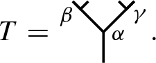
Let $T\in Y_{m}(\Omega )$ and $T'\in Y_{n}(\Omega )$ be two decorated planar binary trees and $\alpha$ an element in $\Omega$. The grafting $\vee _\alpha$ of T and $T'$ on $\alpha$ is the $(n + m + 1)$-decorated planar binary tree $T\vee _\alpha T'\in Y_{m+n+1}(\Omega )$, obtained by joining the roots of T and $T'$ and create a new root, which is decorated by $\alpha$. For any decorated planar binary tree $T\in Y_{n}(\Omega )$ with $n\geqslant 1$, there exist unique elements $T^l\in Y_{k}(\Omega )$, $T^r\in Y_{n-k-1}(\Omega )$ and $\alpha \in \Omega$ such that

$$\begin{aligned} T=T^l\vee _{\alpha }T^r, \end{aligned}$$

where $T^l$ and $T^r$ are the left-hand side of T and the right-hand side of T, respectively. For instance,

A multiplication $*$ on $H_\mathrm{LR}(\Omega )$ with unit | is given recursively on the sum of depth as [14, Sec. 4.3]

$$\begin{aligned} |*T :=T*|:= T\ \text { and } T*T':=T^l\vee _\alpha (T^r*T')+(T*T^{'l})\vee _\beta T^{'r}, \end{aligned}$$

(1)

where $T=T^l\vee _\alpha T^r$ and $T'=T^{'l}\vee _\beta T^{'r}$ are in $Y_\infty (\Omega )$ with $\alpha ,\beta \in \Omega$. Let us agree to fix the notation $*$ to denote the multiplication given in Eq. (1) hereafter.

Example 2.1

We have

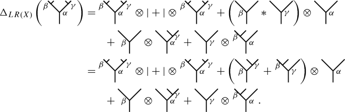
In the undecorated case, the description of the coproduct in the Loday–Ronco Hopf algebra $H_\mathrm{LR}$ was first introduced in [27, Proposition 3.3]. In the decorated case, Foissy [14, Sec. 4.3] equipped the $\mathbf {k}$-algebra $H_\mathrm{LR}(\Omega )$ with a coproduct $\Delta _{LR(\Omega )}$ described recursively on $\mathrm {dep}(T)$ for basis elements $T\in Y_\infty (\Omega )$ as

$$\begin{aligned} \Delta _{LR(\Omega )}(T):=|\otimes | \,\text { if } T=|; \end{aligned}$$

(2)

and for $T = T^l\vee _{\alpha }T^r$,

$$\begin{aligned} \Delta _{LR(\Omega )}(T)&:=\Delta _{LR(\Omega )}(T^l\vee _{\alpha }T^r):=(T^l\vee _{\alpha }T^r)\otimes | \nonumber \\&\quad +(*, \vee _\alpha )\bigl (\Delta _{LR(\Omega )}(T^l)\otimes \Delta _{LR(\Omega )}(T^r)\bigr ), \end{aligned}$$

(3)

where $(*, \vee _\alpha ):=(*\otimes \vee _\alpha )\circ {\tau _{23}}$ and $\tau _{23}$ is the permutation of the second and third tensor factors.

Example 2.2

We have

Foissy [14] also defined linear maps

$$\begin{aligned} \varepsilon _{LR(\Omega )}: H_\mathrm{LR}(\Omega )\rightarrow \mathbf {k}, \quad | \mapsto 1_\mathbf{k}\,\text { and }\, T \mapsto 0 \,\text { for }\, |\ne T\in Y_\infty (\Omega ) \end{aligned}$$

and

$$\begin{aligned} |: \mathbf{k}\rightarrow H_\mathrm{LR}(\Omega ), \quad 1_\mathbf{k}\mapsto |. \end{aligned}$$

Recall [33] that a bialgebra $(H, *_H, 1_H, \Delta , \varepsilon )$ is called $\mathbf {graded}$ if there are $\mathbf {k}$-submodules $H^{(n)}, n\geqslant 0$, of H such that

• (a) $H=\bigoplus _{n=0}^{\infty }H^{(n)}$;

• (b) $H^{(p)}H^{(q)}\subseteq H^{(p+q)}, \, p, q \geqslant 0$; and

• (c) $\Delta (H^{(n)})\subseteq \bigoplus _{p+q=n}H^{(p)}\otimes H^{(q)}, n\geqslant 0$.

Elements of $H^{(n)}$ are called to have degree n. H is called $\mathbf {connected}$ if $H^{(0)}=\mathbf {k}$ and $\ker \varepsilon =\bigoplus _{n\geqslant 1}H^{(n)}$. It is well known that a connected graded bialgebra is a Hopf algebra [32].

Lemma 2.3

[14, Sec. 4.3] [33, Sec. 6.3.5] The quintuple $(H_\mathrm{LR}(\Omega ), *, |, \Delta _{LR(\Omega )}, \varepsilon _{LR(\Omega )})$ is a connected graded bialgebra with grading $H_\mathrm{LR}(\Omega )= \oplus _{n\geqslant 0} \mathbf{k}Y_{n}(\Omega )$ and hence a Hopf algebra.

If $\Omega$ is a singleton set, then $Y_\infty (\Omega )$ is precisely the planar binary trees (without decorations) and one gets the Loday–Ronco Hopf algebra on planar binary trees [27, Thm. 3.1].

2.2 A combinatorial description of $\Delta _{LR(\Omega )}$

Next, we give a combinatorial description of the coproduct $\Delta _{LR(\Omega )}$ by the admissible cut which was introduced by Connes and Kreimer [10] on rooted trees and further studied by Foissy [16] on decorated rooted trees. This notion of cut of rooted trees can be adapted to decorated planar binary trees as follows.

Let $T\in Y_{\infty }(\Omega )$ be a decorated planar binary tree. The edges of T are oriented upwards, from root to leaves. A (non-total) cutc is a choice of edges connecting internal vertices of T. Note that an edge connecting a leaf and an internal vertex is not in a cut. In particular, the empty cut is a cut with the choice of no edges. The cut c is called admissible if any oriented path from a vertex of the tree to the root meets at most one cut edge. For an admissible cut c, cutting each edge in c into two edges, T is sent to a pair $(P^c(T), R^c(T))$, such that $R^c(T)$ is the connected component containing the root of T and $P^c(T)$ is the product of the other connected components with respect to the multiplication $*$ given in Eq. (1), from left to right. The total cut is also added, which is by convention an admissible cut such that

$$\begin{aligned} R^c(T)=| \text { and } P^c(T)=T. \end{aligned}$$

The set of admissible cuts of T is denoted by $\text{ Adm }_*(T)$. Let us note that the empty cut is admissible. Denote by

$$\begin{aligned} \text{ Adm }(T) := \text{ Adm }_*(T) \setminus \{\text{ empty } \text{ cut, } \text{ total } \text{ cut }\}. \end{aligned}$$

Example 2.4

• (a) Consider the decorated planar binary tree

  

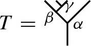
  with $\alpha , \beta , \gamma \in \Omega$. It has $2^{2}$ non-total cuts and one total cut.

  

• (b) Consider the decorated planar binary tree

  

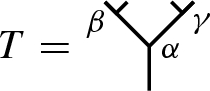
  with $\alpha , \beta , \gamma \in \Omega$. It has $2^{2}$ non-total cuts and one total cut.

  

Remark 2.5

It should be pointed out that our admissible cut is different from the one, which is introduced by Connes–Kreimer on undecorated planar rooted trees [10] and further studied by Foissy on decorated planar rooted trees [16]. For example, under the framework of [16], Foissy gave

The undecorated case can also be found in  [10, Figure 5]. Note that the cutting edge is deleted. However, our admissible cut c cuts each cutting edge into two edges.

Now, we are ready to give a combinatorial description of the coproduct $\Delta _{LR(\Omega )}$.

Theorem 2.6

Let $T \in Y_{\infty }(\Omega )\setminus \{|\}$. Then,

$$\begin{aligned} \Delta _{LR(\Omega )}(T)&=\sum _{c\in \text{ Adm }_*(T)} P^c(T)\otimes R^c(T)=T\otimes |+|\otimes T \nonumber \\&\quad +\sum _{c \in \text{ Adm }(T)} P^c(T) \otimes R^c(T). \end{aligned}$$

(4)

Proof

We prove Eq. (4) by induction on the depth $\mathrm {dep}(T)\geqslant 1$. For the initial step of $\mathrm {dep}(T)=1$, we have

for some $\alpha \in \Omega$. Since

has only one internal vertex and each edge in a cut can’t connect a leaf and an internal vertex, T has only two cuts—the total cut and the empty cut. Thus, $\text{ Adm }_*(T)$ consists of the total cut and the empty cut, and so

For the induction step of $\mathrm {dep}(T)\geqslant 2$, we may write $T = T^l\vee _{\alpha }T^r$ for some $T^l, T^r\in Y_{\infty }(\Omega )$ and $\alpha \in \Omega$. We have two cases to consider.

Case 1.$\mathrm {dep}(T^l)=0$ and $\mathrm {dep}(T^r)\geqslant 1$, or $\mathrm {dep}(T^l)\geqslant 1$ and $\mathrm {dep}(T^r)=0$. Without loss of generality, we consider $\mathrm {dep}(T^l)=0$ and $\mathrm {dep}(T^r)\geqslant 1$. Then, $T^l=|$ and $T = |\vee _{\alpha }T^r$. By Eq. (3),

$$\begin{aligned} \Delta _{LR(\Omega )}(T)&= \ \Delta _{LR(\Omega )}(|\vee _{\alpha }T^r)=(|\vee _{\alpha }T^r)\otimes |\\&\quad +(*, \vee _\alpha )\bigl (\Delta _{LR(\Omega )}(|)\otimes \Delta _{LR(\Omega )}(T^r)\bigr )\\&=\ T\otimes |+(*, \vee _\alpha )\bigl (|\otimes |\otimes \Delta _{LR(\Omega )}(T^r)\bigr )\quad \quad (\text {by Eq.}~(2) )\\&=\ T\otimes |+(*, \vee _\alpha )\bigg (|\otimes |\otimes \Big (T^r\otimes |+|\otimes T^r \\&\quad +\sum _{c \in \text{ Adm }(T^r)} P^c(T^r) \otimes R^c(T^r)\Big )\bigg )\\&\quad \quad \quad (\text {by the induction hypothesis})\\&= T\otimes |+(*, \vee _\alpha )\bigg (|\otimes |\otimes T^r\otimes |+|\otimes |\otimes |\otimes T^r \\&\quad +\sum _{c \in \text{ Adm }(T^r)} |\otimes |\otimes P^c(T^r) \otimes R^c(T^r)\bigg )\\&=\ T\otimes |+(|*T^r)\otimes (|\vee _{\alpha }|)+(|*|)\otimes (|\vee _{\alpha } T^r)\\&\quad +\sum _{c \in \text{ Adm }(T^r)} (|*P^c(T^r)) \otimes (|\vee _{\alpha } R^c(T^r))\\&=\ T\otimes |+ |\otimes (|\vee _{\alpha } T^r)+T^r\otimes (|\vee _{\alpha }|) \\&\quad +\sum _{c \in \text{ Adm }(T^r)} P^c(T^r) \otimes (|\vee _{\alpha } R^c(T^r))\\&=\ T\otimes |+ |\otimes T+\sum _{c \in \text{ Adm }(T)} P^c(T) \otimes R^c(T^r). \end{aligned}$$

Case 2.$\mathrm {dep}(T^l)\geqslant 1$ and $\mathrm {dep}(T^r)\geqslant 1$. Then, $T = T^l\vee _{\alpha }T^r$ with $T^l\ne |$ and $T^r\ne |$. It follows from Eq. (3) that

$$\begin{aligned} \Delta _{LR(\Omega )}(T)&= \Delta _{LR(\Omega )}(T^l\vee _{\alpha }T^r)= (T^l\vee _{\alpha }T^r)\otimes | \nonumber \\&\quad +(*, \vee _\alpha )\bigl (\Delta _{LR(\Omega )}(T^l)\otimes \Delta _{LR(\Omega )}(T^r)\bigr )\nonumber \\&=\ T\otimes |+(*, \vee _\alpha )\biggl (\Big (T^l\otimes |+|\otimes T^l\nonumber \\&\quad +\sum _{c \in \text{ Adm }(T^l)} P^c(T^l) \otimes R^c(T^l)\Big )\nonumber \\&\quad \otimes \Big (T^r\otimes |+|\otimes T^r \nonumber \\&\quad +\sum _{c' \in \text{ Adm }(T^r)} P^{c'}(T^r) \otimes R^{c'}(T^r)\Big )\biggr ) \quad (\text {by the induction hypothesis})\nonumber \\&= T\otimes |+(*, \vee _\alpha )\biggl (T^l\otimes | \otimes T^r\otimes | +T^l\otimes |\otimes |\otimes T^r \nonumber \\&\quad +T^l\otimes |\otimes \sum _{c' \in \text{ Adm }(T^r)} P^{c'}(T^r) \otimes R^{c'}(T^r)\nonumber \\&\quad +|\otimes T^l \otimes T^r\otimes |+|\otimes T^l \otimes |\otimes T^r \nonumber \\&\quad + |\otimes T^l \otimes \sum _{c' \in \text{ Adm }(T^r)} P^{c'}(T^r) \otimes R^{c'}(T^r)\nonumber \\&\quad +\sum _{c \in \text{ Adm }(T^l)} P^c(T^l) \otimes R^c(T^l)\otimes T^r\otimes | \nonumber \\&\quad +\sum _{c \in \text{ Adm }(T^l)} P^c(T^l)\otimes R^c(T^l) \otimes |\otimes T^r \nonumber \\&\quad +\sum _{c \in \text{ Adm }(T^l)} \sum _{c' \in \text{ Adm }(T^r)}P^{c}(T^l)\otimes R^{c}(T^l)\otimes P^{c'}(T^r) \otimes R^{c'}(T^r)\biggr ) \nonumber \\&= \ T\otimes |+(T^l*T^r) \otimes (| \vee _\alpha |) +T^l\otimes (| \vee _\alpha T^r)\nonumber \\&\quad +\sum _{c' \in \text{ Adm }(T^r)} (T^l*P^{c'}(T^r)) \otimes ( |\vee _\alpha R^{c'}(T^r)) \nonumber \\&\quad +T^r\otimes (T^l\vee _{\alpha } |)+|\otimes (T^l\vee _\alpha T^r) \nonumber \\&\quad +\sum _{c' \in \text{ Adm }(T^r)} P^{c'}(T^r) \otimes (T^l\vee _\alpha R^{c'}(T^r))\nonumber \\&\quad +\sum _{c \in \text{ Adm }(T^l)}( P^c(T^l) *T^r)\otimes (R^c(T^l)\vee _\alpha |)\nonumber \\&\quad +\sum _{c \in \text{ Adm }(T^l)} P^c(T^l) \otimes ( R^c(T^l)\vee _\alpha T^r) \nonumber \\&\quad +\sum _{c \in \text{ Adm }(T^l)} \sum _{c' \in \text{ Adm }(T^r)}(P^c(T^l)*P^{c'}(T^r)) \otimes (R^c(T^l)\vee _\alpha R^{c'}(T^r))\nonumber \\&=\ T\otimes |+|\otimes T+(T^l*T^r) \otimes (| \vee _\alpha |) +T^l\otimes (| \vee _\alpha T^r)\nonumber \\&\quad +T^r\otimes (T^l\vee _{\alpha } |)\nonumber \\&\quad +\sum _{c' \in \text{ Adm }(T^r)} (T^l*P^{c'}(T^r)) \otimes ( |\vee _\alpha R^{c'}(T^r))\nonumber \\&\quad +\sum _{c' \in \text{ Adm }(T^r)} P^{c'}(T^r) \otimes (T^l\vee _\alpha R^{c'}(T^r)) \nonumber \\&\quad +\sum _{c \in \text{ Adm }(T^l)}( P^c(T^l) *T^r)\otimes (R^c(T^l)\vee _\alpha |) \nonumber \\&\quad +\sum _{c \in \text{ Adm }(T^l)} P^c(T^l) \otimes ( R^c(T^l)\vee _\alpha T^r) \nonumber \\&\quad +\sum _{c \in \text{ Adm }(T^l)} \sum _{c' \in \text{ Adm }(T^r)}(P^c(T^l)*P^{c'}(T^r)) \otimes (R^c(T^l)\vee _\alpha R^{c'}(T^r)). \end{aligned}$$

(5)

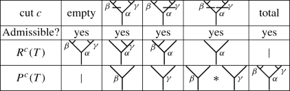
We may draw the decorated planar binary tree T graphically as

Then, all kinds of admissible cuts in $\text{ Adm }(T)$ can be illustrated graphically as:

Note that the last eight terms in Eq. (5) are precisely corresponding to the eight kinds of admissible cuts in $\text{ Adm }(T)$. Thus,

$$\begin{aligned} \Delta _{LR(\Omega )}(T)=\Delta _{LR(\Omega )}(T^l\vee _{\alpha }T^r)=T\otimes |+|\otimes T+\sum _{c \in \text{ Adm }(T)} P^c(T) \otimes R^c(T). \end{aligned}$$

This completes the proof. $\square$

Example 2.7

• (a) Consider the planar binary tree

  

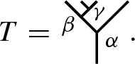
  By Theorem 2.6 and Example 2.4 (a), we have

  

• (b) Let

  

  It follows from Theorem 2.6 and Example 2.4 (b) that

  

Observe that the results in (a) and (b) are consistent with the corresponding ones in Example 2.2.

As a direct consequence of Theorem 2.6, we may give another proof of the following result, which was obtained in [14, Sec. 4.3] and [33, Sec. 6.3.5].

Corollary 2.8

For each $n\geqslant 0$,

$$\begin{aligned} \Delta _{LR(\Omega )}(\mathbf{k}Y_n(\Omega )) \subseteq \bigoplus _{p+q = n} \mathbf{k}Y_p(\Omega ) \otimes \mathbf{k}Y_q(\Omega ). \end{aligned}$$

Proof

Let $T\in Y_n(\Omega )$. Denote by $\mathrm{Int}(T)$ the set of interior vertices of T. Then, $|\mathrm{Int}(T)| = n$. For an admissible cut c in $\text{ Adm }_*(T)$, write

$$\begin{aligned} P^c(T) = T_1 *\cdots *T_k\,\text { and }\, R^c(T) = T_{k+1}\,\text { for some }\ k\geqslant 0. \end{aligned}$$

Here, we use the convention that $P^c(T) = |$ when $k=0$. By [14, Sec. 4.3], the number of interior vertices of each summand in $T_1 *\cdots *T_k$ is $\sum _{i=1}^k |\mathrm{Int}(T_i)|$. So, by Theorem 2.6, the number of interior vertices of each summand in $\Delta _{LR(\Omega )}(T)$ is

$$\begin{aligned} \sum _{i=1}^{k} |\mathrm{Int}(T_i)| +|\mathrm{Int}(T_{k+1})| = |\mathrm{Int}(T)| = n, \end{aligned}$$

whence

$$\begin{aligned} \Delta _{LR(\Omega )} \in \bigoplus _{p+q = n} \mathbf{k}Y_p(\Omega ) \otimes \mathbf{k}Y_q(\Omega ), \end{aligned}$$

as required. $\square$

Remark 2.9

By Theorem 2.6, the fact that $H_\mathrm{LR}(\Omega )$ is a connected graded bialgebra is obvious.

2.3 Subcoalgebras of coalgebra of decorated planar binary trees

In this subsection, we only consider the aforementioned coalgebraic structure on decorated planar binary trees and show that $H_\mathrm{LR}(\Omega )$ is a strictly graded coalgebra.

Let C be a coalgebra. If there exists a family of $\mathbf{k}$-submodules $\{C^{(n)}\mid n\geqslant 0\}$ of C such that

• (a) $C=\bigoplus _{n\geqslant 0}C^{(n)}$;

• (b) $\varepsilon (C^{(n)})=0$ , $n\ne 0$; and

• (c) $\Delta (C^{(n)})\subseteq \bigoplus _{p+q=n}C^{(p)}\otimes C^{(q)}, n\geqslant 0$,

then C is called a graded coalgebra. If in particular,

$$\begin{aligned} C^{(0)}\cong \mathbf{k} \text{ and } C^{(1)}=P(C), \end{aligned}$$

then C is said to be a strictly graded coalgebra [1, Chap. 4.1], where P(C) is the set of primitive elements of C.

Definition 2.10

 [1, Chap. 3.1] Let C be a coalgebra.

• (a) A subcoalgebra M of C is called a simple subcoalgebra if it does not have any subcoalgebras other than 0 and M.

• (b) C is called irreducible if C has only one simple subcoalgebra.

• (c) C is called pointed if all simple subcoalgebras of C are one dimensional.

Lemma 2.11

 [1, Chap. 4.1] A strictly graded coalgebra is a pointed irreducible coalgebra.

Narrowing our attention to the coalgebraic structure of $H_\mathrm{LR}(\Omega )$, we obtain

Theorem 2.12

The coalgebra $(H_\mathrm{LR}(\Omega ), \Delta _{LR(\Omega )}, \varepsilon _{LR(\Omega )})$ is a strictly graded coalgebra with the grading $H_\mathrm{LR}(\Omega )= \oplus _{n\geqslant 0} \mathbf{k}Y_{n}(\Omega )$ and hence has only one simple subcoalgebra $\mathbf{k}\{|\}$.

Proof

By Lemma 2.3, $H_\mathrm{LR}(\Omega )= \oplus _{n\geqslant 0} \mathbf{k}Y_{n}(\Omega )$ is a graded coalgebra. Since $Y_0(\Omega ) = Y_0 = \{|\}$, we have $\mathbf {k}Y_{0}(\Omega )=\mathbf {k}$. Furthermore,

is the set of primitive elements of $H_\mathrm{LR}(\Omega )$ by Theorem 2.6. Thus, $H_\mathrm{LR}(\Omega )$ is a strictly graded coalgebra. By Lemma 2.11, $H_\mathrm{LR}(\Omega )$ has only one simple subcoalgebra. Then, the result follows from that $\mathbf {k}Y_{0}(\Omega )=\mathbf{k}\{|\}$ is a simple subcoalgebra of $H_\mathrm{LR}(\Omega )$. $\square$

Remark 2.13

Summing up, the coradical of the Hopf algebra $H_\mathrm{LR}(\Omega )$ (that is to say the sum of all its simple coalgebra) is $\mathbf {k}\{|\}$.

3 Free cocycle $\vee _\Omega$-Hopf algebras of decorated planar binary trees

In this section, based on the binary grafting operations $\vee _\alpha$ on $H_\mathrm{LR}(\Omega )$ with $\alpha \in \Omega$, we introduce the concept of a $\vee$-algebra and more generally a $\vee _\Omega$-algebra, leading to the emergence of $\vee _\Omega$-bialgebras and $\vee _\Omega$-Hopf algebras. Further when a $\vee$-cocycle condition is involved, cocycle $\vee _\Omega$-bialgebras and cocycle $\vee _\Omega$-Hopf algebras are also introduced. We finally show that $H_\mathrm{LR}(\Omega )$ is a free cocycle $\vee _\Omega$-Hopf algebra.

3.1 Free $\vee _\Omega$-algebras of decorated planar binary trees

In this subsection, we equip the space $H_\mathrm{LR}(\Omega )$ of planar binary trees decorated by a nonempty set $\Omega$ with a free $\vee _\Omega$-algebra structure. Let us first recall the concept of operated algebras.

Definition 3.1

[19, Sec. 1.2]

• (a) An operated algebra is an algebra A together with a (linear) operator $P: A\rightarrow A$.

• (b) An $\Omega$-operated algebra is an algebra A together with a set of (linear) operators $P_{\alpha }: A\rightarrow A$, $\alpha \in \Omega$.

Motivated by the above definition and Eq. (1), we introduce $\vee$-algebras.

Definition 3.2

• (a) A $\vee$-algebra is an algebra $(A, *_A, 1)$ together with a binary operation $\vee :A\otimes A \rightarrow A$ such that, for $a=a_1\vee a_2$ and $a'=a_1'\vee a_2'$ in A,

  $$\begin{aligned} a*_A a'=a_1 \vee (a_2*_{A} a')+(a*_A a_1')\vee a_2'. \end{aligned}$$

  More generally, let $\Omega$ be a nonempty set.

• (b) A $\vee _\Omega$-algebra is an algebra $(A, *_A, 1_A)$ equipped with a set of binary operations

  $$\begin{aligned} \vee _\Omega := \{\vee _\alpha :A\otimes A \rightarrow A \mid \alpha \in \Omega \} \end{aligned}$$

  such that

  $$\begin{aligned} a*_{A} a'=a_1 \vee _{\alpha } (a_2*_{A} a')+(a*_{A} a_1')\vee _{\alpha '} a_2', \end{aligned}$$

  (6)

  where $a=a_1 \vee _\alpha a_2$ and $a'=a_1'\vee _{\alpha '} a_2'$ in A with $\alpha , \alpha '\in \Omega$. We denote such a $\vee _\Omega$-algebra by $(A, *_A, 1_A, \vee _\Omega )$.

• (c) Let $(A, *_A, 1_A, \vee _\Omega )$ and $(A', *_{A'}, 1_{A'}, \vee '_\Omega )$ be two $\vee _\Omega$-algebras. A linear map $\phi : A\rightarrow A'$ is called a $\vee _\Omega$-algebra morphism if $\phi$ is an algebra homomorphism such that $\phi \circ \vee _\alpha = \vee '_\alpha \circ (\phi \otimes \phi )$ for each $\alpha \in \Omega$.

• (d) A free $\vee _\Omega$-algebra on a set X is a $\vee _\Omega$-algebra $(A, *_A, 1_A, \vee _\Omega )$ together with a set map $j:X\rightarrow A$ with the property that, for any $(A', *_{A'}, 1_{A'}, \vee '_\Omega )$ and a set map $\phi :X\rightarrow A'$, there exists a unique $\vee _\Omega$-algebra morphism $\overline{\phi }:A\rightarrow A'$ such that $\overline{\phi } \circ j=\phi$.

Remark 3.3

Let us emphasize that $\vee$-algebras are different from operated algebras: the $\vee$-algebra is an algebra equipped with a binary operation satisfying Eq. (6), but the operated algebra is an algebra equipped with a unary operation.

Example 3.4

It follows from Eq. (1) that $(H_\mathrm{LR}(\Omega ), *, |, \vee _\Omega )$ is a $\vee _\Omega$-algebra. Indeed, it is a free $\vee _\Omega$-algebra with a universal property (see Theorem 3.5 below).

The significant role of the binary grafting $\vee _{\Omega }$ is clarified by the following universal property.

Theorem 3.5

The quadruple $(H_\mathrm{LR}(\Omega ), *, |, \vee _{\Omega })$ is the free $\vee _{\Omega }$-algebra on the empty set, that is, the initial object in the category of $\vee _{\Omega }$-algebras. More precisely, for any $\vee _\Omega$-algebra $A=(A, *_A, 1_A, \vee _{A, \Omega })$, there exists a unique $\vee _\Omega$-algebra morphism $\overline{\phi }: H_\mathrm{LR}(\Omega )\rightarrow A$.

Proof

(Uniqueness). Suppose that $\overline{\phi }: H_\mathrm{LR}(\Omega ) \rightarrow A$ is a $\vee _\Omega$-algebra morphism. We prove the uniqueness of $\overline{\phi }(T)$ for basis elements $T\in Y_{\infty }(\Omega )$ by induction on $\mathrm {dep}(T)\geqslant 0$. For the initial step of $\mathrm {dep}(T)=0$, we have $T = |$ and $\overline{\phi }(T) = \overline{\phi }(|) = 1_A$. For the induction step of $\mathrm {dep}(T)\geqslant 1$, we may write $T = T_1\vee _{\alpha } T_2$ for some $\alpha \in \Omega$ and then

$$\begin{aligned} \overline{\phi }(T) =&\, \overline{\phi }(T_1\vee _{\alpha } T_2) = \overline{\phi }\circ \vee _\alpha (T_1,T_2) = \vee _{A,\alpha }\circ (\overline{\phi }\otimes \overline{\phi })(T_1, T_2) \\ =&\vee _{A, \alpha }\bigl (\overline{\phi }(T_1)\otimes \overline{\phi }(T_2)\bigr )=\overline{\phi }(T_1)\vee _{A, \alpha }\overline{\phi }(T_2). \end{aligned}$$

Here, $\overline{\phi }(T_1)$ and $\overline{\phi }(T_2)$ are determined uniquely by the induction hypothesis and so $\overline{\phi }(T)$ is unique.

(Existence). Define a linear map ${\overline{\phi }}: H_\mathrm{LR}(\Omega ) \rightarrow A$ recursively on depth $\mathrm {dep}(T)$ for $T\in Y_{\infty }(\Omega )$ by assigning

$$\begin{aligned} \overline{\phi }(|) :=1_A\,\text { and }\, \overline{\phi }(T) :=\overline{\phi }(T_1\vee _\alpha T_2):=\overline{\phi }(T_1)\vee _{A,\alpha }\overline{\phi }(T_2), \end{aligned}$$

(7)

where $T=T_1\vee _\alpha T_2$ for some $T_1, T_2\in Y_\infty (\Omega )$ and $\alpha \in \Omega$. Then, for any $T_1, T_2\in Y_{\infty }(\Omega )$, we have

$$\begin{aligned} \overline{\phi }\circ \vee _\alpha (T_1,T_2)&=\overline{\phi }(T_1\vee _\alpha T_2)=\overline{\phi }(T_1)\vee _{A, \alpha }\overline{\phi }(T_2)=\vee _{A, \alpha }\bigl (\overline{\phi }(T_1)\otimes \overline{\phi }(T_2) \bigr ) \\&= \vee _{A, \alpha } \circ (\overline{\phi }\otimes \overline{\phi })(T_1, T_2) \end{aligned}$$

and so

$$\begin{aligned} \overline{\phi }\circ \vee _\alpha = \vee _{A, \alpha }\circ (\overline{\phi }\otimes \overline{\phi }). \end{aligned}$$

We are left to check that

$$\begin{aligned} \overline{\phi } (T*T')=\overline{\phi }(T)*_{A}\overline{\phi }(T')\,\text { for any }\, T, T'\in Y_{\infty }(\Omega ). \end{aligned}$$

(8)

We proceed to prove Eq. (8) by induction on the sum of depths $\mathrm {dep}(T)+ \mathrm {dep}(T')\geqslant 0$. For the initial step of $\mathrm {dep}(T)+ \mathrm {dep}(T') = 0$, we have $T = T'=|$ and

$$\begin{aligned} \overline{\phi } (T*T')&=\overline{\phi }(|*|)=\overline{\phi }(|)=1_A=1_A*_{A} 1_A=\overline{\phi }(|)*_{A}\overline{\phi }(|) \\&= \overline{\phi }(T) *_A \overline{\phi }(T'). \end{aligned}$$

For the induction step of $\mathrm {dep}(T)+ \mathrm {dep}(T') \geqslant 1$, if $\mathrm {dep}(T) = 0$ or $\mathrm {dep}(T') = 0$, without loss of generality, letting $\mathrm {dep}(T) = 0$, then $T=|$ and

$$\begin{aligned} \overline{\phi } (T*T')&=\overline{\phi }(|*T')=\overline{\phi }(T')= 1_A *_A\overline{\phi }(T')= \overline{\phi }(|) *_A \overline{\phi }(T')\\&=\overline{\phi }(T) *_A \overline{\phi }(T'). \end{aligned}$$

So, we may assume that $\mathrm {dep}(T), \mathrm {dep}(T')\geqslant 1$ and write

$$\begin{aligned} T = T_1 \vee _\alpha T_2 \text { and } T' = T'_1 \vee _\beta T'_2\,\text { for some }\, \alpha ,\beta \in \Omega . \end{aligned}$$

Hence,

$$\begin{aligned} \overline{\phi }(T*T')&=\overline{\phi }\bigl (T_1\vee _\alpha (T_2*T')+(T*T_1')\vee _\beta T_2'\bigr )\quad (\text {by Eq.}~(1) )\\&=\overline{\phi }\bigl (T_1\vee _\alpha (T_2*T')\bigr )+\overline{\phi }\bigl ((T*T_1')\vee _\beta T_2'\bigr )\quad (\text {by }\overline{\phi } \text { being linear}) \\&=\overline{\phi }(T_1)\vee _{A,\alpha } \overline{\phi }(T_2*T')+\overline{\phi }(T*T_1')\vee _{A,\beta }\overline{\phi }(T_2') \quad (\text {by Eq.}~(7) )\\&=\overline{\phi }(T_1)\vee _{A,\alpha }\bigl (\overline{\phi }(T_2)*_{A}\overline{\phi }( T')\bigr )+\bigl (\overline{\phi }(T)*_{A}\overline{\phi }( T_1')\bigr )\vee _{A,\beta } \overline{\phi }(T_2')\\&\quad \quad \quad \quad (\text {by the induction hypothesis})\\&=\overline{\phi }(T_1)\vee _{A,\alpha }\Bigl (\overline{\phi }(T_2)*_{A} \bigl (\overline{\phi }( T_1')\vee _{A,\beta } \overline{\phi }(T_2')\bigr )\Bigr )\\&\quad +\Bigl ( \bigl (\overline{\phi }(T_1)\vee _{A,\alpha }\overline{\phi }(T_2) \bigr ) *_{A}\overline{\phi }( T_1')\Bigr )\vee _{A,\beta } \overline{\phi }(T_2')\\&\quad \quad \quad \quad (\text {by Eq.}~(7))\\&=\bigl (\overline{\phi }(T_1)\vee _{A,\alpha }\overline{\phi }(T_2)\bigr )*_{A}\bigl (\overline{\phi }( T_1')\vee _{A,\beta } \overline{\phi }(T_2')\bigr )\quad (\text {by Eq.}~(6) ) \\&=\overline{\phi }(T_1\vee _{\alpha } T_2)*_{A}\overline{\phi }( T_1'\vee _{\beta } T_2')\quad (\text {by Eq.}~(7) )\\&=\overline{\phi }(T)*_{A}\overline{\phi }(T'), \end{aligned}$$

as required. This completes the proof. $\square$

3.2 Free cocycle $\vee _\Omega$-Hopf algebras of decorated planar binary trees

In this subsection, we prove that $H_\mathrm{LR}(\Omega )$ is the free cocycle $\vee _\Omega$-Hopf algebra on the empty set. Let us first pose the following concepts which are motivated from the binary grafting operations $\{\vee _\alpha \mid \alpha \in \Omega \}$ characterized in Eq. (1) and the coproduct $\Delta _{LR(\Omega )}$ given in Eq. (3).

Definition 3.6

• (a) A $\vee _\Omega$-bialgebra (resp. $\vee _\Omega$-Hopf algebra) is a bialgebra (resp. Hopf algebra) $(H, *_H, 1_H, \Delta _H, \varepsilon _H )$ which is also a $\vee _\Omega$-algebra $(H,*_H, 1_H,\vee _{\Omega })$.

• (b) Let $(H,\, \vee _{\Omega })$ and $(H',\,\vee '_{\Omega })$ be two $\vee _\Omega$-bialgebras (resp. $\vee _\Omega$-Hopf algebras). A linear map $\phi : H\rightarrow H'$ is called a $\vee _\Omega$-bialgebra morphism (resp. $\vee _\Omega$-Hopf algebra morphism) if $\phi$ is a bialgebra (resp. Hopf algebra) morphism such that ${\phi }\circ \vee _{\alpha } = \vee '_{\alpha }\circ ({\phi }\otimes {\phi })$ for $\alpha \in \Omega$.

Involved with an analogy of the Hochschild 1-cocycle condition [15], we pose

Definition 3.7

• (a) An $\Omega$-cocycle $\vee _\Omega$-bialgebra or simply a cocycle $\vee _\Omega$-bialgebra is a $\vee _\Omega$-bialgebra $(H, *_H, 1_H, \Delta _H, \varepsilon _H, \vee _\Omega )$ satisfying the following $\vee$-cocycle condition: for any $\alpha \in \Omega$ and $h,h'\in H,$

  $$\begin{aligned} \Delta _H (h \vee _\alpha h') = (h \vee _\alpha h') \otimes 1_H +(*_H, \vee _\alpha )\bigl (\Delta _H(h)\otimes \Delta _H(h')\bigr ), \end{aligned}$$

  (9)

  where $(*_H,\vee _\alpha ):=(*_H \otimes \vee _H)\circ {\tau _{23}}$ and $\tau _{23}$ is the permutation of the second and third tensor factor. If the bialgebra in a cocycle $\vee _\Omega$-bialgebra is a Hopf algebra, then it is called a cocycle $\vee _\Omega$-Hopf algebra.

• (b) A free cocycle $\vee _\Omega$-bialgebra on a set X is a cocycle $\vee _\Omega$-bialgebra $(H, *_H, 1_H,\Delta _H,\varepsilon _H, \vee _\Omega )$ together with a set map $j: X\rightarrow H$ with the property that for any cocycle $\vee _\Omega$-bialgebra $(H', *_{H'}, 1_{H'}, \Delta _{H'}, \varepsilon _{H'}, \vee '_{\Omega })$ and any set map $\phi : X \rightarrow H'$, there exists a unique $\vee _\Omega$-bialgebra morphism $\overline{\phi }:H \rightarrow H'$ such that $\overline{\phi } \circ j =\phi$. The concept of a free cocycle $\vee _\Omega$-Hopf algebra is defined in the same way.

When $\Omega$ is a singleton set, the subscript $\Omega$ in Definitions 3.2 and 3.7 will be suppressed for simplicity.

The following result gives a family of coideals of a cocycle $\vee _\Omega$-bialgebra. Recall that a submodule I in a coalgebra $(C, \Delta , \varepsilon )$ is called a coideal if $I\subseteq \ker \varepsilon$ and $\Delta (I) \subseteq I\otimes C + C\otimes I$. A biideal of a bialgebra A is a submodule of A which is both an ideal and a coideal of A.

Proposition 3.8

Let $(H, *_{H}, 1_H, \Delta _{H}, \varepsilon _H, \vee _{\Omega })$ be a cocycle $\vee _\Omega$-bialgebra and C a coideal of H. Then, we have the following.

• (a) $H\vee _{\alpha } H := \{h_1 \vee _\alpha h_2 \mid h_1, h_2\in H\}$ is a coideal of H for each $\alpha \in \Omega$.

• (b) The ideal generated by C is a biideal.

Proof

(a) Let $\alpha \in \Omega$. We first show $H\vee _\alpha H\subseteq \ker \varepsilon _H$. Let

$$\begin{aligned} h =h_1\vee _{\alpha }h_2 \in H\vee _\alpha H \,\text { with }\, h_1, h_2 \in H. \end{aligned}$$

Using Sweedler notation, we can write

$$\begin{aligned} \Delta _H(h_1)=\sum _{(h_1)}h_{1(1)}\otimes h_{1(2)}\, \text { and }\, \Delta _H(h_2)=\sum _{ (h_2)}h_{2(1)}\otimes h_{2(2)}. \end{aligned}$$

Then,

$$\begin{aligned} h_1\vee _{\alpha }h_2&=\ (\varepsilon _H \otimes \mathrm{id})\circ \Delta _{H}(h_1\vee _{\alpha }h_2)\quad \quad \quad (\text {by the counicity})\\&= (\varepsilon _H \otimes \mathrm{id})\Big ((h_1 \vee _\alpha h_2) \otimes 1_H \\&\quad +(*_H, \vee _\alpha )\bigl (\Delta _H(h_1)\otimes \Delta _H(h_2)\bigr )\Big )\quad (\text {by Eq.}~(9))\\&=\ \varepsilon _H (h_1 \vee _\alpha h_2) \otimes 1_H+(\varepsilon _H \otimes \mathrm{id})\circ (*_H, \vee _\alpha )\\&\quad \left( \bigg (\sum _{(h_1)}h_{1(1)}\otimes h_{1(2)}\bigg )\otimes \bigg (\sum _{ (h_2)}h_{2(1)}\otimes h_{2(2)}\bigg )\right) \\&=\ \varepsilon _H (h_1 \vee _\alpha h_2) \otimes 1_H+(\varepsilon _H \otimes \mathrm{id})\circ (*_H, \vee _\alpha )\\&\quad \left( \sum _{(h_1), (h_2)}h_{1(1)}\otimes h_{1(2)}\otimes h_{2(1)}\otimes h_{2(2)}\right) \\&=\ \varepsilon _H (h_1 \vee _\alpha h_2) \otimes 1_H+(\varepsilon _H \otimes \mathrm{id})\\&\quad \left( \sum _{(h_1), (h_2)}(h_{1(1)}*_{H} h_{2(1)})\otimes (h_{1(2)}\vee _{\alpha }h_{2(2)}) \right) \\&\quad \quad \quad (\text {by } (*_H,\vee _\alpha ):=(*_H \otimes \vee _\alpha )\circ {\tau _{23}})\\&= \varepsilon _H (h_1 \vee _\alpha h_2) \otimes 1_H\\&\quad + \sum _{(h_1), (h_2)}\varepsilon _H(h_{1(1)}*_{H} h_{2(1)})\otimes (h_{1(2)}\vee _{\alpha }h_{2(2)}) \\&= \varepsilon _H (h_1 \vee _\alpha h_2) \otimes 1_H \\&\quad + \sum _{(h_1), (h_2)}\Big (\varepsilon _H(h_{1(1)})*_{\mathbf{k}} \varepsilon _H(h_{2(1)})\Big ) (h_{1(2)}\vee _{\alpha }h_{2(2)}) \\&= \varepsilon _H (h_1 \vee _\alpha h_2) \otimes 1_H\\&\quad + \sum _{(h_1), (h_2)}\Big (\varepsilon _H(h_{1(1)})*_{\mathbf{k}} h_{1(2)}\Big ) \vee _{\alpha } \Big ( \varepsilon _H(h_{2(1)}) *_{\mathbf{k}} h_{2(2)}\Big ) \\&= \varepsilon _H (h_1 \vee _\alpha h_2) \otimes 1_H \\&\quad +h_1 \vee _{\alpha } h_2\quad (\text {by the counicity}), \end{aligned}$$

which implies

$$\begin{aligned} \varepsilon _H (h_1 \vee _\alpha h_2)\otimes 1_H=0\,\text { and so }\, \varepsilon _H (h_1 \vee _\alpha h_2)=0. \end{aligned}$$

We next show

$$\begin{aligned} H\vee _\alpha H\subseteq (H\vee _\alpha H)\otimes H + H\otimes (H\vee _\alpha H). \end{aligned}$$

Indeed, for any $h_1\vee _\alpha h_2\in H\vee _\alpha H$,

$$\begin{aligned} \Delta _{H}(h_1\vee _{\alpha }h_2)&=(h_1\vee _{\alpha }h_2)\otimes 1_{H}\\&\quad +(*_H, \vee _{\alpha })\bigl (\Delta _H(h_1)\otimes \Delta _H(h_2)) \quad (\text {by Eq.}~(9))\\&= (h_1\vee _{\alpha }h_2)\otimes 1_{H}+(*_H, \vee _{\alpha }) \\&\quad \bigg ( \sum _{(h_1), (h_2)}(h_{1(1)}\otimes h_{1(2)})\otimes (h_{2(1)}\otimes h_{2(2)}) \bigg )\\&= (h_1\vee _{\alpha }h_2) \otimes 1_{H}\\&\quad +\sum _{(h_1), (h_2)}(h_{1(1)}*_H h_{2(1)})\otimes (h_{1(2)}\vee _{\alpha }h_{2(2)})\\&\in (H\vee _\alpha H) \otimes H+ H\otimes (H\vee _\alpha H). \end{aligned}$$

Thus, $H\vee _\alpha H$ is a coideal.

(b) Suppose that I is the ideal generated by C. Then, we can write $I=H*_{H}C*_{H}H$ and so

$$\begin{aligned} \Delta _{H}(I)&=\Delta _{H}(H*_{H}C*_{H}H) = \Delta _{H}(H)*_{H}\Delta _{H}(C)*_{H}\Delta _{H}(H)\\&\subseteq (H\otimes H)*_{H}(C\otimes H+H\otimes C)*_{H}(H\otimes H)\\&= (H*_{H}C*_{H}H) \otimes (H *H*H) \\&\quad + (H*H*H) \otimes (H*_{H}C*_{H}H)\\&=I\otimes H+H\otimes I. \end{aligned}$$

Thus I is a biideal of H. $\square$

As a consequence of Proposition 3.8 (a), we obtain a family of coideals of $H_\mathrm{LR}(\Omega )$.

Corollary 3.9

The $H_\mathrm{LR}(\Omega ) \vee _{\alpha } H_\mathrm{LR}(\Omega )$ is a coideal of $H_\mathrm{LR}(\Omega )$ for each $\alpha \in \Omega$.

Proof

It follows from Proposition 3.8 (a). $\square$

Now we are ready for our main result of this section.

Theorem 3.10

Let $\Omega$ be a nonempty set.

• (a) The sextuple $(H_\mathrm{LR}(\Omega ), *, |, \Delta _{LR(\Omega )}, \varepsilon _{LR(\Omega )}, \vee _\Omega )$ is the free cocycle $\vee _\Omega$-bialgebra on the empty set, that is, the initial object in the category of cocycle $\vee _\Omega$-bialgebras.

• (b) The sextuple $(H_\mathrm{LR}(\Omega ), *, |, \Delta _{LR(\Omega )}, \varepsilon _{LR(\Omega )}, \vee _\Omega )$ is the free cocycle $\vee _\Omega$-Hopf algebra on the empty set, , that is, the initial object in the category of cocycle $\vee _\Omega$-Hopf algebras.

Proof

(a) It follows from Lemma 2.3 that $(H_\mathrm{LR}(\Omega ), *, |, \Delta _{LR(\Omega )}, \varepsilon _{LR(\Omega )})$ is a bialgebra. Furthermore, the $(H_\mathrm{LR}(\Omega ), *, |, \Delta _{LR(\Omega )}, \varepsilon _{LR(\Omega )}, \vee _\Omega )$ is a $\vee _\Omega$-bialgebra by Eq. (1) and a cocycle $\vee _\Omega$-bialgebra by Eq. (3).

We are left to show the freeness of $H_\mathrm{LR}(\Omega )$. For this, let $(H, *_{H}, 1_H, \Delta _{H}, \varepsilon _H, \vee '_{\Omega })$ be an arbitrary cocycle $\vee _\Omega$-bialgebra. In particular, $(H, *_H, 1_H, \vee '_\Omega )$ is a $\vee _\Omega$-algebra. So, by Theorem 3.5, there exists a unique algebra homomorphism $\overline{\phi }: H_\mathrm{LR}(\Omega )\rightarrow H$ such that

$$\begin{aligned} \overline{\phi }\circ \vee _\alpha = \vee '_\alpha \circ (\overline{\phi }\otimes \overline{\phi }) \text { for any } \alpha \in \Omega . \end{aligned}$$

(10)

It remains to check the following two points:

$$\begin{aligned} \Delta _{H} \circ \overline{\phi } (T)&=(\overline{\phi } \otimes \overline{\phi }) \circ \Delta _{LR(\Omega )}(T), \end{aligned}$$

(11)

$$\begin{aligned} \varepsilon _H \circ \overline{\phi }(T)&= \varepsilon _{LR(\Omega )}(T) \, \text { for all } \, T\in Y_\infty (\Omega ). \end{aligned}$$

(12)

We prove Eq. (11) by induction on $\mathrm {dep}(T)\geqslant 0$. For the initial step of $\mathrm {dep}(T)=0$, we have $T=|$ and

$$\begin{aligned} \Delta _{H} \circ \overline{\phi } (T)&= \Delta _{H} \circ \overline{\phi } (|)=\Delta _{H} (1_H)=1_H\otimes 1_H=\overline{\phi } (|)\otimes \overline{\phi }(|)\\&=(\overline{\phi }\otimes \overline{\phi })(|\otimes |)= (\overline{\phi }\otimes \overline{\phi })\circ \Delta _{LR(\Omega )}(|) = (\overline{\phi }\otimes \overline{\phi })\circ \Delta _{LR(\Omega )}(T). \end{aligned}$$

For the induction step of $\mathrm {dep}(T)\geqslant 1$, we may write $T = T_1\vee _\alpha T_2$ for some $T_1, T_2\in Y_{\infty }(\Omega )$ and $\alpha \in \Omega$. Using the Sweedler notation,

$$\begin{aligned} \Delta _{LR(\Omega )}(T_1)=\sum _{(T_1)}T_{1(1)}\otimes T_{1(2)} \text { and } \Delta _{LR(\Omega )}(T_2)=\sum _{(T_2)}T_{2(1)}\otimes T_{2(2)}. \end{aligned}$$

(13)

Then,

$$\begin{aligned}&\Delta _{H} \circ \overline{\phi }(T)\\&=\Delta _{H} \circ \overline{\phi }(T_1\vee _\alpha T_2)=\Delta _{H} \bigl (\overline{\phi }(T_1)\vee '_{\alpha } \overline{\phi }(T_2)\bigr ) \quad (\text {by Eq.}~(10))\\&=\big (\overline{\phi }(T_1)\vee '_{\alpha } \overline{\phi }(T_2)\big )\otimes 1_{H}+(*_{H},\vee '_{\alpha })\\&\quad \Bigl (\Delta _{H}\bigl (\overline{\phi }(T_1)\bigr )\otimes \Delta _{H}\bigl (\overline{\phi }(T_2)\bigr )\Bigr )\quad (\text {by Eq.}~(9))\\&=\overline{\phi }(T_1\vee _\alpha T_2)\otimes 1_{H}+(*_{H},\vee '_{\alpha })\bigg (\Bigl ((\overline{\phi }\otimes \overline{\phi })\Delta _{LR(\Omega )}(T_1)\Bigr )\\&\quad \otimes \Bigl ((\overline{\phi }\otimes \overline{\phi })\Delta _{LR(\Omega )}(T_2)\Bigr )\bigg )\\&\quad \quad \quad \quad (\text {by Eq.}~(10) \text { and the induction hypothesis)}\\&=(\overline{\phi }\otimes \overline{\phi })\Bigl ((T_1\vee _\alpha T_2)\otimes |\Bigr )+(*_{H},\vee '_{\alpha })\bigg (\Bigl ((\overline{\phi }\otimes \overline{\phi })\Delta _{LR(\Omega )}(T_1)\Bigr )\\&\quad \otimes \Bigl ((\overline{\phi } \otimes \overline{\phi })\Delta _{LR(\Omega )}(T_2)\Bigr )\bigg )\\&=(\overline{\phi }\otimes \overline{\phi })\Bigl ((T_1\vee _\alpha T_2)\otimes |\Bigr )+(*_{H},\vee '_{\alpha }) \bigg ( \sum _{(T_1),(T_2)}\Bigl (\overline{\phi }(T_{1(1)})\otimes \overline{\phi }(T_{1(2)})\Bigr )\\&\quad \otimes \Bigl (\overline{\phi }(T_{2(1)})\otimes \overline{\phi }(T_{2(2)})\Bigr ) \bigg )\\&\quad \quad \quad \quad \quad \quad (\text {by Eq.}~(13))\\&=(\overline{\phi }\otimes \overline{\phi })\Bigl ((T_1\vee _\alpha T_2)\otimes |\Bigr )+\sum _{(T_1),(T_2)}\Bigl (\overline{\phi }(T_{1(1)})*_{H} \overline{\phi }(T_{2(1)})\Bigr )\\&\quad \otimes \Bigl (\overline{\phi }(T_{1(2)})\vee '_{\alpha } \overline{\phi }(T_{2(2)})\Bigr )\\&=(\overline{\phi }\otimes \overline{\phi })\Bigl ((T_1\vee _\alpha T_2)\otimes |\Bigr )\\&\quad +\sum _{(T_1),(T_2)}\overline{\phi }(T_{1(1)}*T_{2(1)})\otimes \overline{\phi }(T_{1(2)}\vee _\alpha T_{2(2)})\\&\quad \quad \quad \quad \quad (\text {by }\overline{\phi } \text { being an algebra homomorphism and Eq.}~(10))\\&=(\overline{\phi }\otimes \overline{\phi })\Bigl ((T_1\vee _\alpha T_2)\otimes |\Bigr )\\&\quad +(\overline{\phi }\otimes \overline{\phi }) \bigg ( \sum _{(T_1),(T_2)}(T_{1(1)}*T_{2(1)})\otimes (T_{1(2)}\vee _\alpha T_{2(2)}) \bigg )\\&=(\overline{\phi }\otimes \overline{\phi })\Bigl ((T_1\vee _\alpha T_2)\otimes |\Bigr )\\&\quad + (\overline{\phi }\otimes \overline{\phi }) \circ (*, \vee _\alpha )\Bigl (\Delta _{LR(\Omega )}(T_1)\otimes \Delta _{LR(\Omega )}(T_2)\Bigr )\\&=(\overline{\phi }\otimes \overline{\phi })\biggl ((T_1\vee _\alpha T_2)\otimes |+(*, \vee _\alpha )\Bigl (\Delta _{LR(\Omega )}(T_1)\otimes \Delta _{LR(\Omega )}(T_2)\Bigr )\biggr )\\&=(\overline{\phi }\otimes \overline{\phi }) \circ \Delta _{LR(\Omega )}(T_1\vee _\alpha T_2)\\&=(\overline{\phi }\otimes \overline{\phi }) \circ \Delta _{LR(\Omega )}(T). \end{aligned}$$

We next prove Eq. (12). If $T=|$, then

$$\begin{aligned} \varepsilon _H \circ \overline{\phi }(T) = \varepsilon _H \circ \overline{\phi }(|)=\varepsilon _H(1_H)=1_{\mathbf {k}}=\varepsilon _{LR(\Omega )}(|). \end{aligned}$$

If $T\ne |$, then T can be written as $T = T_1\vee _\alpha T_2$ for some $T_1, T_2\in Y_{\infty }(\Omega )$ and $\alpha \in \Omega$. By Eq. (10),

$$\begin{aligned} \varepsilon _H \circ \overline{\phi }(T)=\varepsilon _H \circ \overline{\phi }(T_1\vee _\alpha T_2)=\varepsilon _H \bigl (\overline{\phi }(T_1)\vee '_\alpha \overline{\phi }(T_2)\bigr )= 0 =\varepsilon _{LR(\Omega )}(T), \end{aligned}$$

(14)

where the second last step employs Proposition 3.8 (a). This completes the proof of Item (a).

(b) By Lemma 2.3, $(H_\mathrm{LR}(\Omega ), *, |, \Delta _{LR(\Omega )}, \varepsilon _{LR(\Omega )})$ is a Hopf algebra. It is further a $\vee _\Omega$-Hopf algebra by Eq. (1) and a cocycle $\vee _\Omega$-Hopf algebra by Eq. (3). Then, Item (b) follows from Item (a) and the well-known fact that any bialgebra morphism between two Hopf algebras is compatible with the antipodes [37, Lem. 4.04]. $\square$

Taking $\Omega$ to be a singleton set in Theorem 3.10, all planar binary trees in $H_\mathrm{LR}(\Omega )$ are decorated by the same letter. In other words, planar binary trees in $H_\mathrm{LR}(\Omega )$ have no decorations in this case and that are precisely the planar binary trees in the classical Loday–Ronco Hopf algebra $H_\mathrm{LR}$. So

Corollary 3.11

• (a) The classical Loday–Ronco Hopf algebra $H_\mathrm{LR}$ is the free cocycle $\vee$-bialgebra on the empty set, that is, the initial object in the category of cocycle $\vee$-bialgebras.

• (b) The classical Loday–Ronco Hopf algebra $H_\mathrm{LR}$ is the free cocycle $\vee$-Hopf algebra on the empty set, that is, the initial object in the category of cocycle $\vee$-Hopf algebras.

Proof

It follows from Theorem 3.10 by taking $\Omega$ to be a singleton set. $\square$

References

Abe, E.: Hopf algebras. Translated from the Japanese by Hisae Kinoshita and Hiroko Tanaka. Cambridge Tracts in Mathematics, vol. 74. Cambridge University Press, Cambridge-New York (1980)
Aguiar, M., Sottile, F.: Structure of the Loday–Ronco Hopf algebra of trees. J. Algebra 295, 473–511 (2006)
Bokut, L.A., Chen, Y., Qiu, J.: Gröbner-Shirshov bases for associative algebras with multiple operators and free Rota–Baxter algebras. J. Pure Appl. Algebra 214, 89–110 (2010)
Brouder, C., Frabetti, A.: QED Hopf algebras on planar binary trees. J. Algebra 267, 298–322 (2003)
Brouder, C., Frabetti, A., Menous, F.: Combinatorial Hopf algebras from renormalization. J. Algebraic Combin. 32, 557–578 (2010)
Chapoton, F.: A Hopf operad of forests of binary trees and related finite-dimensional algebras. J. Algebraic Combin. 20, 311–330 (2004)
Chapoton, F.: Operads and algebraic combinatorics of trees. Sém. Lothar. Combin. 58, 2 (2008)
Chapoton, F., Frabetti, A.: From Quantum Electrodynamics to Posets of Planar Binary Trees. In: Ebrahimi-Fard, K., Marcolli, M., van Suijlekom, W.D. (eds.) Combinatorics and Physics. Contemporary Mathematics, vol. 539. American Mathematical Society, Providence, RI (2011)
Chapoton, F., Livernet, M.: Pre-Lie algebras and the rooted trees operad. Int. Math. Res. Not. IMRN 8, 395–408 (2001)
Connes, A., Kreimer, D.: Hopf algebras, renormalization and non-commutative geometry. Comm. Math. Phys. 199(1), 203–242 (1998)
Connes, A., Kreimer, D.: Renormalization in quantum field theory and the Riemann–Hilbert problem. I. The Hopf algebra structure of graphs and the main theorem. Comm. Math. Phys. 210, 249–273 (2000)
Ebrahimi-Fard, K., Guo, L., Kreimer, D.: Spitzer’s identity and the algebraic Birkhoff decomposition in pQFT. J. Phys. A: Math. Gen. 37, 11037–11052 (2004)
Foissy, L.: Les algèbres de Hopf des arbres enracinés décorés. I, (French) [Hopf algebras of decorated rooted trees, I]. Bull. Sci. Math. 126(3), 193–239 (2002)
Foissy, L.: Les algèbres de Hopf des arbres enracinés décorés. II, (French) [Hopf algebras of decorated rooted trees, II]. Bull. Sci. Math. 126(4), 249–288 (2002)
Foissy, L.: Introduction to Hopf algebra of rooted trees (2013). http://loic.foissy.free.fr/pageperso/p11.pdf
Foissy, L.: Classification of systems of Dyson–Schwinger equations of the Hopf algebra of decorated rooted trees. Adv. Math. 224, 2094–2150 (2010)
Gao, X., Guo, L.: Rota’s Classification Problem, rewriting systems and Gröbner–Shirshov bases. J. Algebra 470, 219–253 (2017)
Grossman, R., Larson, R.G.: Hopf-algebraic structure of families of trees. J. Algebra 126, 184–210 (1989)
Guo, L.: Operated semigroups, Motzkin paths and rooted trees. J. Algebraic Combin. 29, 35–62 (2009)
Guo, L.: An Introduction to Rota–Baxter Algebra. International Press, Somerville (2012)
Guo, L., Paycha, S., Zhang, B.: Algebraic Birkhoff factorization and the Euler–Maclaurin formula on cones. Duke Math. J. 166, 537–571 (2017)
Holtkamp, R.: Comparison of Hopf algebras on trees. Arch. Math. (Basel) 80, 368–383 (2003)
Hohlweg, C., Lange, C., Thomas, H.: Permutahedra and generalized associahedra. Adv. Math. 226, 608–640 (2011)
Kreimer, D.: On the Hopf algebra structure of perturbative quantum field theories. Adv. Theor. Math. Phys. 2, 303–334 (1998)
Kreimer, D., Panzer, E.: Renormalization and Mellin transforms. In: Schneider, C., Blümlein, J. (eds.) Computer Algebra in Quantum Field Theory. Texts Monographs in Symbolic Computation, pp. 195–223. Springer, Vienna (2013)
Kurosh, A.G.: Free sums of multiple operator algebras. Sib. Math. J. 1, 62–70 (1960)
Loday, J.-L., Ronco, M.O.: Hopf algebra of the planar binary trees. Adv. Math. 139, 293–309 (1998)
Loday, J.-L.: une version non commutative des algèbre de Lie: les algèbres de Leibniz. Enseign. Math. 39, 269–293 (1993)
Loday, J.-L.: Dialgebras. In: Loday, J.-L., Frabetti, A., Chapoton, F., Goichot, F. (eds.) Dialgebras and Related Operads. Lecture Notes in Mathematics, vol. 1763, pp. 7–66. Springer, Berlin (2001)
Loday, J.-L.: Realization of the Stasheff polytope. Arch. Math. (Basel) 83, 267–278 (2004)
Loday, J.-L., Vallette, B.: Algebraic operads. Grundlehren der Mathematischen Wissenschaften, vol. 346. Springer, Heidelberg (2012)
Manchon, D.: Hopf algebras, from basics to applications to renormalization. Comptes-rendus des Rencontres mathematiques de Glanon 2001 (2003). arXiv:math.QA/0408405
Manchon, D.: Hopf algebras in renormalisation. In: Hazewinkel, M. (ed.) Handbook of Algebra, vol. 5, pp. 365–427. Elsevier/North-Holland, Amsterdam (2008)
Moerdijk, I.: On the Connes–Kreimer construction of Hopf algebras. Contemp. Math. 271, 311–321 (2001)
Ronco, M.: Eulerian idempotents and Milnor–Moore theorem for certain non-cocommutative Hopf algebras. J. Algebra 254, 152–172 (2002)
Stanley, R. P.: Enumerative Combinatorics. Cambridge Studies in Advanced Mathematics, vol. 1, no. 49. Cambridge University Press, Cambridge (1997)
Sweedler, M.E., Otto, F.: Hopf Algebras. Mathematics Lecture Note Series. W. A. Benjamin Inc., New York (1969)
Zhang, T.J., Gao, X., Guo, L.: Hopf algebras of rooted forests, cocycles, and free Rota–Baxter algebras. J. Math. Phys. 57, 101701 (2016)
Acknowledgements
This work was supported by the National Natural Science Foundation of China (Grant No. 11771191, 11501267 and 11861051), Fundamental Research Funds for the Central Universities (Grant No. lzujbky-2017-162) and the Natural Science Foundation of Gansu Province (Grant No. 17JR5RA175). We thank Prof. Foissy for helpful discussion, and Proposition 3.8 is inspired by the email communication with him.
Author information
Authors and Affiliations
Corresponding author
Additional information
Publisher's Note
Springer Nature remains neutral with regard to jurisdictional claims in published maps and institutional affiliations.
Rights and permissions
About this article
Cite this article
Zhang, Y., Gao, X. Hopf algebras of planar binary trees: an operated algebra approach. J Algebr Comb 51, 567–588 (2020). https://doi.org/10.1007/s10801-019-00885-8
Received:
Accepted:
Published:
Issue Date:
DOI: https://doi.org/10.1007/s10801-019-00885-8