
Abstract
Dynamic site response is usually implemented using an equivalent-linear approach through analyses based on time-histories or random vibration theory (RVT). In the RVT approach the input motion is characterized in the frequency domain by means of Fourier Amplitude Spectra (FAS) or power spectral densities so that the need for selecting/developing multiple suitable time-histories is avoided. Nevertheless, past studies have found that RVT may produce results that differ significantly from empirically determined site amplification functions and from the time history approach. This work is aimed to further understand the potential differences in the results from RVT and time-histories based approaches by performing a comprehensive numerical evaluation that takes into account the effect of the input intensity level, input spectral shape, site conditions, and the methodology used to produce the input FAS. The results obtained corroborate that RVT over-predictions occur mainly at the site fundamental frequencies and are larger for relatively soft soil deposits with significant impedance contrast at the soil/rock interface. However, in the soft site evaluated the magnitude of the over-prediction was rather insensitive to the increase in the inelastic demand, conversely, the over-prediction in the stiffer site increased as the site softened due to the rising inelastic demand.
Introduction
In the seismic design and/or assessment of many critical structures, like nuclear power plants (NPPs), the seismic input is defined from a probabilistic seismic hazard analysis (PSHA) as a uniform hazard response spectrum (UHRS) at the rock outcrop. A seismic wave transmission analysis (i.e., site response analysis) is then performed to obtain the UHRS at the free-field ground surface (or at any elevation required). The dynamic site response analysis is usually implemented using an equivalent-linear (EQL) approach through methodologies based either on time-histories or, more recently, random vibration theory (RVT). Both approaches are currently accepted by the US Nuclear Regulatory Commission (US-NRC [1].
In the time-histories based method, a suitable set of ground motions should be selected and scaled or modified to obtain records that match the design spectrum. Due to the variability of the properties within the input motions, a relatively large number of simulations needs to be performed to obtain a consistent estimate of the site response [2]. Alternately, the RVT approach can be used to avoid the selection, scaling and matching of time-histories input motions. This approach uses a single input motion defined in the frequency domain as either a Fourier Amplitude Spectrum (FAS) or a Power Spectral Density (PSD) compatible with the design spectrum. However, past studies have found that, in some cases, prediction of the site amplification at the site natural frequency by RVT analysis can be 20–50% larger than with time-histories approach. Moreover, it has been noticed that sites with low fundamental frequency and settled on hard rock produce the largest over-predictions [3, 4].
This work is aimed to further understand the potential differences in the results from RVT and time-histories based approaches by performing a comprehensive numerical evaluation that takes into account the effect of the input intensity level, input spectral shape, site conditions, and the methodology used to produce the input FAS. It should be noticed that different implementations of the RVT based approach have been proposed [5]. In this work the RVT methodology used is the one proposed by Ozbey and Rathje [4] and implemented in the software Strata [6]. This methodology employs a FAS as input and the peak factor formulation from Cartwright and Longuet-Higgins [7]. Other methodologies that use a PSD as input and/or a different peak factor formulation (e.g. Deng and Ostadan [8) are not evaluated.
The analyses performed can be seen as an extension of the work presented by Kottke and Rathje [3], in fact, the two sites analyzed were extracted from there. Important differences worth mention are:
-
1.
The seismic input for the time-histories based analyses were developed in compliance with NRC requirements [1]. That is, spectrum compatible records were developed based on the modification of recorded accelerograms. In Kottke and Rathje [3], the analyses were performed using stochastically simulated time-series motions with a specified strong motion duration. As a result, it is expected that the seismic input used in this work would have a larger variability in terms of frequency content and duration.
-
2.
Different methodologies to generate the spectrum compatible FAS used as input in the RVT based approach are evaluated.
-
3.
Different design spectra and levels of intensity are used to develop the seismic input, so that the influence of the spectral shape and soil inelastic demand can be investigated.
Time-histories and RVT based equivalent-linear site response
Incorporation of soil non-linearity in seismic site response analyses is fundamental since soil deposits exhibit non-linear hysteretic behavior even at low levels of strain demand. The more rigorous approach to capture the nonlinear soil behavior is to perform time domain nonlinear (NL) site response analyses. When performing NL analyses special care is required in the development of the model: selection of soil constitutive model and its parameters, damping model and profile discretization. While this type of analyses has gain popularity over the last years, in practice most site response studies are performed using one dimensional frequency domain equivalent linear (EQL) procedures due to their robustness, simplicity, flexibility and low computational requirements [9]. In EQL site-response analyses, the propagation of the wave through the soil layers is modeled using transfer functions and the soil nonlinearity is incorporated through the use of strain-compatible soil properties (shear modulus and damping). Therefore, an iterative scheme needs to be implemented where the soil properties are updated based on the strain level until the maximum strain for all layers converge. The conditions for which one-dimensional EQL and NL site response analyses results are large enough to be of practical significance have been recently studied in Kim et al. [10] and are out of the scope of this work.
Time-histories and RVT approaches are both grounded on the EQL method, the main difference is in the fashion the seismic input is defined. In the first method, the input consists of time histories while for the RVT based approach, the input is represented by a FAS or PSD. In both cases to comply with most design codes requirements the inputs need to be compatible with a design response spectrum. In the time-histories approach, the variability of ground motions may generate significant different responses and levels of nonlinearity [3], thus, a number of inputs to perform the analysis several times are required to obtain a steady average site response. Since the input is defined in the time domain, Fast Fourier Transforms (FFT) are used to convert it to the frequency domain, where all the calculations are performed. The resulting time history at the ground surface is obtained applying the inverse FFT to the Fourier coefficients estimated after the application of the transfer functions.
In the RVT approach, a single analysis is performed using a compatible FAS or PSD as input. As the input is already in the frequency domain, the EQL analysis can be performed without having to use the FFT. However, the use of the inverse FFT to get the ground surface time history is not possible because although the amplitude of the Fourier Spectrum is available, the phase angle is not. Instead, random vibration theory is applied to estimate other response values, such as peak ground and spectral accelerations. Moreover, Parseval’s theorem is used to compute the root-mean-square acceleration, a rms , Eq. (1):
where a(t) is the signal in the time domain, GMD rms is the root mean square of the ground motion duration [e.g. Liu and Pezeshk [11], A(f) is the Fourier amplitude at frequency f and m o is the zero-order spectral moment of the FAS, Eq. (2):
the time domain peak values are then estimated by multiplying the a rms by a peak factor (pf). The computer code Strata implements the formulation by Cartwright and Longuet-Higgins [7]:
where ξ is a bandwidth factor, N e is the number of extrema, and m i is the ith order spectral moment of the FAS. It shall be noticed that many models of the statistical distribution of the peak factor have been proposed. More recently, Wang and Rathje [12], found that the use of the Vanmarcke [13] peak factor model provides RVT estimates of site amplification closer to those from the time-histories approach. Nevertheless, significant over-prediction was still noticed for specific combinations of site dynamic properties and seismic input frequency content. A detailed description of the RVT procedure can be found somewhere else [4].
Generation of the seismic input
Selection and development of spectrally matched records
Three sets of 100 spectrum compatible acceleration time series were developed from historic earthquake records, each set aiming to match a different target spectrum. The seed records were obtained from the Next Generation Attenuation of Ground Motions (NGA-West2) database [14] and its selection was based on the overall spectral shape resemblance between the records response spectra and the target design spectrum [15]. The initial level of matching of the seed records was estimated using the root mean square deviation (D rms ) between the spectral amplitudes, Eq. (6). The scale factor a, Eq. (7), is applied to the record spectral accelerations (S αR ) to reduce the spectral amplitude misfit with the target (S αT ) and N is the number of periods where the spectra are evaluated.
Once the seed records are selected, they are modified to make them compatible with the design spectrum while complying with Appendix F of R.G. 1.208 [1]. A Continuous Wavelet Transform (CWT) based algorithm was used to generate the spectrum compatible records [16]. This algorithm decomposes the original record into detail functions (functions with a very dominant frequency and modulated amplitude) and reconstruct the signal through an iterative procedure that independently scale these detail functions to obtain an average match with the target spectrum [17]. This methodology has been shown to preserve the main characteristics of the seed records (e.g. Perez-Rivera and Montejo [18]).
The target design spectrum to which the input motions are made compatible is varied to evaluate the influence of the input spectral shape on the results from time-histories and RVT analyses. Three spectral shapes with different dominant frequencies and bandwidths are used. The first target spectrum is extracted from section “Conclusion” of RG 1.208 [1] and represents a typical UHRS at the outcrop rock, it is denominated NRC spectrum for further identification. The second target is a deterministic spectrum for a magnitude 6.5 earthquake in a strike slip fault with a distance to rupture of 50 km for a site with Vs30 = 370 m/s developed using the tools available at the PEER NGA Ground Motion Database [14], it will be identified as NGA spectrum. Finally, the third spectrum is characterized by high levels of energy at high frequencies and it will be identified as NUC spectrum (to denote it is representative of the Nuclear industry practice). This spectrum was developed for a representative Central/Eastern U.S. site as part of the response initiatives taken by the U.S. nuclear industry after the Fukushima earthquake [19]. An example of the resulting compatible records and response spectra is presented in Fig. 1. The results shown corresponds to a record from the 1994 Northridge earthquake (NGA# 1008) made compatible to the NRC spectrum. Figure 2 shows each of the target spectra scaled to a peak ground acceleration (PGA) of 0.3 g, the pseudo acceleration spectra (PSA) for the records generated are also presented in this figure along with each set median PSA. The FAS and significant durations (D 5–75 ) from all the records are also presented in this figure. The D 5–75 is calculated as the time interval at which 5 and 75% of the Arias intensity is reached. It is noticed that although each set of 100 records shares approximately the same response spectrum, the variability in the FAS and durations is quite significant within each set.

Example of a compatible record (left) and its response spectrum (right)

Top to bottom: pseudo-acceleration response spectra, Fourier amplitude spectrum, and significant duration (D5–75). Left to right: results corresponding to the NRC, NGA and NUC target spectra
Development of the spectrum compatible FAS
A critical first step in RVT site response analyses is the development of an appropriate input FAS, which often need to be defined consistent with a uniform hazard spectrum (UHS) to comply with code requirements. Four different approaches to generate the compatible FAS were evaluated in this work:
-
1.
Inverse RVT (IRVT): The IRVT procedure proposed by Rathje et al. [20] uses extreme value statistics, the characteristics of single-degree-of-freedom oscillator transfer functions, and a spectral ratio correction to develop the Fourier amplitude spectra. This procedure is implemented in the computer program Strata [6] and requires of empirical approximations and an iterative scheme to converge. In addition to the target spectrum, a consistent strong motion duration is required as input to the inversion process. Since the sets of compatible records used for the time history approach exhibited a wide range of strong motion durations, settling on a single duration value to use in the IRVT methodology is not obvious. An optimal duration is estimated by generating a number of FAS for different strong motion durations. Each FAS is compared via D rms with the average FAS from the 100 spectrum compatible records previously developed, the optimal duration is set as the one that generated the FAS with the minimum D rms . The results obtained are presented in Fig. 3 and compared with the average significant duration from the 100 records. It is seen that the optimal durations are very close to the average D 5–75 .
Fig. 3 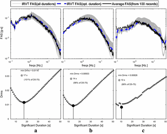
Estimation of the optimal duration for IRVT: Top figures show the IRVT FAS obtained for different durations and bottom figures show their corresponding D rms when compared against the average FAS from the set of 100 spectrum compatible series time-series. Left to right: results corresponding to the NRC, NGA and NUC target spectra
-
2.
Damping modification factors (DMF): DMF are commonly used to adjust elastic response spectral values corresponding to 5% of viscous damping to other damping levels. Based on the observation that the FAS of a ground motion is very similar to the undamped velocity spectrum, DMF were used to convert the average 5% pseudo velocity spectrum (PSV) of the 100 records to an undamped velocity spectrum which is used as the input FAS. The DMF where calculated using the expression proposed by Hatzigeorgiou [21], Eq. (8), with the coefficient values c i suggested for spectrum compatible records. Although this expression was developed for damping ratios (ζ) between 0.5 and 50%, following an analysis similar to the one performed to obtain the optimal duration for the IRVT procedure, it was found that using the coefficients for 0.2% provided the closest match to the average FAS from the 100 spectrum compatible records in each set (Fig. 4).
Fig. 4 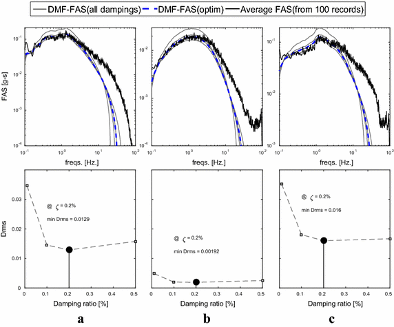
Estimation of the optimal damping ratio for the DMF approach. Top figures show the resulting FAS using DMF with different damping values and bottom figures show their corresponding D rms when compared against the average FAS from the set of 100 spectrum compatible series time-series. Left to right: results corresponding to the NRC, NGA and NUC target spectra
$$DMF\left( {T,\zeta } \right) = 1 + \left( {\zeta - 5} \right)\left[ {1 + c_{1} ln\left( \zeta \right) + c_{2} \left( {ln\left( \zeta \right)} \right)^{2} } \right]\left[ {c_{3} + c_{4} ln\left( T \right) + c_{5} \left( {ln\left( T \right)} \right)^{2} } \right]$$(8) -
3.
Using an empirical relationship: the conversion is performed directly through a duration dependent empirical relationship between FAS and 5% PSA intended mainly for spectrum compatible records, Montejo and Vidot-Vega [23, 24], Eq. (9):
$$\frac{FAS}{5\% PSA} = \left[ {a_{1} \left( {D_{5 - 75} } \right)^{{a_{2} }} + a_{3} } \right]*f^{{\left[ {b_{1} \left( {D_{5 - 75} } \right)^{{b_{2} }} + b_{3} } \right]}}$$(9)where a 1 = 0.0512, a 2 = 0.4920, a 3 = 0.1123, b 1 = − 0.5869, b 2 = − 0.2650 and b 3 = − 0.4580.
-
4.
Average FAS from a set of spectrum compatible records: The fourth approach to estimate the input FAS was to simply take the average FAS from the 100 compatible records in each set. It is clear that this approach goes against the essence of the RVT procedure, however, it was implemented to investigate the influence of the specified FAS in the results and whether the differences with the time-histories approach could be partially attributed to the specification of the FAS. Figure 5 summarizes the results from all four approaches used to develop the spectrum compatible input FAS.
Fig. 5 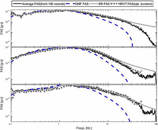
Spectrum compatible input FAS obtained using the 4 different approaches. Top to bottom: results corresponding to the NRC, NGA and NUC spectra


Numerical comparison of the site response procedures
In order to investigate the significance of site conditions on the site response, two different sites used in [2, 3] for the same purpose, were selected. The first site is the Sylmar County Hospital parking lot (SCH) which is located in San Fernando Valley of Southern California and consists of 90 m of alluvium over rock, with shear wave velocity varying from 250 to 760 m/s in the bedrock (no significant impedance contrast). The second site is Calvert Cliffs (CC) located on the coast of Chesapeake Bay in Maryland. This site has over 750 m of alternating layers of sand and clay/silt, with the shear wave velocity varying form 241–2804 m/s in the bedrock for a large impedance contrast at the soil/rock interface. The detailed characteristics of both sites can be found in [2]. The shear velocity profiles and linear-elastic transfer functions (TF) for each site are shown in Fig. 6. A first-mode natural frequency of 1.7 Hz for the SCH site and 0.25 Hz for the CC site are identified.

Shear velocity profiles (a) and elastic transfer functions (b) for the 2 sites studied
Site response analyses using both time-history and RVT based methods are performed using the software Strata [6]. Several analyses are conducted by varying the input intensity level, input spectral shape and site conditions to calculate the amplification function for each case, defined as the ratio between spectral accelerations (AF = S a_out /S a_in ). To evaluate the differences in the results from the time-histories and RVT approaches, the median AF predicted from the 100 time histories (AFTH) and the AF predicted using RVT (AFRVT) is compared by using the ratio between them (αAF = AFRVT/AFTH).
The median AFs obtained by the time-histories approach for each site, target spectrum and level of intensity are presented in Fig. 7. These can be seen as the “target” AFs that would be used to calculate the ratios αAF used to evaluate the RVT results. Three levels of seismic intensity are evaluated that correspond to average PGAs of 0.01, 0.3 and 0.6 g—which are aimed to study 3 different performance levels of the soil deposit: mostly elastic, moderate nonlinearity and highly nonlinear. It is seen that the augment in the soil inelastic demand caused by the increasing intensity in the seismic input is reflected in the AFs by a shift in the site fundamental frequency (softening of the soil deposit) and a response mostly dominated by the first mode (higher modes are attenuated). There is also a slight reduction on the fundamental frequency magnitude of amplification at increasing levels of inelastic demand. Nevertheless, it shall be noticed that as nonlinear effects become more significant (e.g. the 0.6 g case), the response obtained from the EQL method may deviate significantly from the expected one and a full nonlinear analysis in the time domain is more appropriate (e.g. Hashash et al. [9]; Rosario et al. [22]). Moreover, the nonlinear effects were less noticeable in the CC site, presumably due to the large depth of the site controlling its behavior [3]. Finally, it is also noticed that the shape of the spectra used as target did not influence the AFs obtained.

Median AFs from the time-histories approach for the SCH site using NRC (a), NGA (b) and NUC (c) spectra; and for the CC site using NRC (d), NGA (e) and NUC (f) spectra
A sample of the RVT site response results are presented in Fig. 8. The results are presented in the form of AFs for both sites, the three intensity levels and the four different methodologies used to generate the input FAS. The median AFs from the time-histories approach are also presented for comparison purposes as well as the αAF. Due to space constrains only the results obtained when using the NGA spectrum are presented, however, the results obtained for the other two spectra were very similar and lead to the same conclusions. Key remarks from Fig. 8 can be summarized as follows:

AFs and αAFs obtained using inputs compatible with the NGA spectrum. Top figures show the results for the SCH site at PGAs average values of 0.01 g (a), 0.3 g (b) and 0.6 g (c). Bottom figures show the results for the and CC site at 0.01 g (d), 0.3 g (e) and 0.6 g (f)
-
Regarding the site influence: As depicted by Kottke and Rathje [3], the largest over-predictions are obtained at the fundamental frequencies of the soft soil with significant impedance contrast (CC site). The over-prediction at this site reached values of 24% compared to a maximum value of 11.30% in the SCH site.
-
Regarding the methodology used to generate the input FAS: The magnitude of the over-prediction at the sites fundamental frequency was practically the same independent of the methodology used to generate the input FAS. At higher frequencies the AFs obtained from the different input FAS start to differ, especially for the DMF methodology that consistently over-predict the AFs at frequencies larger than ~ 5 Hz.
-
Regarding the level of inelastic demand: For the stiffer site (SCH), the over-predictions at the site natural frequencies are seen to slightly increase as the inelastic demand in the soil increases (Table 1). However, in the deep-soft site evaluated (CC), the level of over-prediction at the fundamental frequency was rather insensitive to the level of inelastic demand. It is also noticed that for larger frequencies (> 1 Hz), there is a tendency to under predict the response as the level of inelastic demand increases.
Table 1 Maximum over-predictions for the SCH and CC sites at different levels of intensity
It shall be noticed that the term “over-prediction” is used to compare how larger the amplifications predicted by the RVT approach are with respect to the predicted by the time series-based approach. While the estimates from the time series-based approach are not the “exact solution”, this is a well stablished and widely used methodology that comprises less approximations than the RVT approach, and therefore it is used as target for comparison purposes.
Evaluation of previously proposed correction factors
Kottke and Rathje [3], have suggested that one of the potential reasons for the over-predictions is the site-response induced increase in significant duration of the motion at the surface. When using the RVT method, this increase in duration is not taken into account, only the input ground motion duration is used. A review of the RVT formulation shows that duration is inversely proportional to the spectral acceleration (Eq. 1). That is, if the increase in duration is ignored, the resulting accelerations will tend to be larger than the ones calculated using the time-histories based approach. To account for this issue, Kottke and Rathje [3] proposed a rather simple fix: modify the AF computed using RVT by dividing by the square root of the observed duration ratio (D surf5–75 /D in5–75 ). Where the D 5–75 values are the [5–75]% significant durations of the responses (to the surface and input motions) of SDOF oscillators with a natural frequency set at the same frequency values used to calculate the AFs. In the work by Kottke and Rathje [3], these ratios were used to correct the predictions based on elastic analyses but their applicability to EQL analyses were no explored. In this work, the same concept was applied to EQL analyses, Fig. 9 summarizes all of the duration ratios obtained for both sites and all input spectra and intensity levels evaluated. The linear elastic case at an input intensity of 0.01 g was also evaluated and is denoted as LE in Fig. 9.

Duration ratios for the SCH site (top figures) and the CC site (bottom figures) for all levels of intensity and input spectra. Left to right: results corresponding to the NRC, NGA and NUC spectra
The duration ratios fluctuated between 0.6 and 2, verifying that there is mostly an increase in the duration. Nevertheless, the duration remained mainly constant in the lower frequency range (< 1 Hz) where most of the sites fundamental frequencies are located. The increment in duration is more evident at frequencies larger than 1 Hz, having its peak value close to 10 Hz. Moreover, as the level of inelastic demand increases in the soil deposit, larger duration ratios are found. It is also noticed that the softer site (CC) exhibits larger variability in the duration ratios. As expected, the ratios obtained at 0.01 g from EQL and LE approaches are quite similar and remain very close to 1 over the whole range of frequencies evaluated. In general, the shape of the duration ratios obtained largely differ from those presented in Kottke and Rathje [3], which follows the same shape of the over-prediction ratios (αAF, Fig. 8). Figures 10 and 11 shows the result of applying the calculated correction factors for both sites, in the sake brevity only the results obtained using the NGA spectrum as input are presented, but similar results were obtained for the other spectral shapes. As expected the use of the correction factors was not successful. Since the correction factors were ~ 1 at the frequency range where most of the sites fundamental frequencies were located, the over-prediction magnitudes remained basically the same. Moreover, at larger frequencies (> 1 Hz) correcting by duration ratios induced an undesirable reduction of αAF, causing now large underpredictions specially at high levels of seismic demand.

Corrected αAF for the CC site and NGA input spectrum: Elastic analysis at 0.01 g (a), EQL at 0.01 g (b), EQL at 0.3 g (c) and EQL at 0.6 g (d)

Corrected αAF for the SCH site and NGA input spectrum: Elastic analysis at 0.01 g (a), EQL at 0.01 g (b), EQL at 0.3 g (c) and EQL at 0.6 g (d)
Conclusions
Over the last years, the nuclear industry has been switching to the RVT-based approach to EQL site response analysis as an alternative to the time-histories method. In theory, RVT would require of only one analysis to obtain the mean amplification function for a site and input spectrum. This may represent substantial computational savings when compared to the traditional time-histories approach, where a relatively large set of input motions needs to be constructed in order to run the several analyses required to obtain a stable mean response. The savings increase dramatically when the studies require that site-property variability be taken into account via Monte Carlo simulation [1]. This work extended the study by Kottke and Rathje [3] by using different design spectra and levels of intensity, so that the influence of the spectral shape and degree of soil inelastic demand can be investigated. Moreover, the development of the input data-set for the time-history base analyses is significantly different, in the study by Kottke and Rathje [3] the input motions were developed using stochastically simulated time-series motions with a specified strong motion duration. In this work, spectrum compatible records were developed based on the modification of recorded accelerograms to comply with current NRC requirements. Therefore, the input motions used in this work would have a larger variability in terms of frequency content and duration. From the results obtained it can be concluded that:
-
As previous studies suggested, over-predictions in the AFs occur mainly at the site fundamental frequencies and the magnitude of the over-prediction is larger for relatively soft soil deposits with significant impedance contrast at the soil/rock interface.
-
The shape of the design spectrum does not seem to influence in the differences between the results from the RVT and time-histories approach.
-
The magnitude of the over-prediction was found to be insensitive to the methodology used to develop the input FAS.
-
In soft sites the magnitude of the over-prediction could be rather insensitive to increments in the inelastic demand, conversely, in stiffer sites the over-prediction may increase as the site softens due to the rising inelastic demand.
-
The correction procedure proposed in [3] for LE analyses was found not to work properly when the seismic input exhibit larger variability independent of the type of analysis performed (EL or EQL).
References
United States Nuclear Regulatory Commission (USNRC) (2007) Nuclear regulatory guide 1.208: a performance-based approach to define the site-specific earthquake ground motion. United States Nuclear Regulatory Commission, Washington
Kottke AR (2010) A comparison of seismic site response methods. Dissertation, The University of Texas at Austin, Texas
Kottke AR, Rathje EM (2013) Comparison of time series and random-vibration theory site-response methods. Bull Seismol Soc Am 103(3):2111–2127
Ozbey MC, Rathje EM (2006) Site-specific validation of random vibration theory-based seismic site response analysis. J Geotech Geoenviron Eng 132(7):911–922
Graizer V (2011) Treasure Island geotechnical array—case study for site response analysis, In: Proceedings of the 4th IASPEI/IAEE international symposium: effects of surface geology on seismic motions, Santa Barbara, California
Kottke AR, Rathje EM (2010). Strata. https://nees.org/resources/strata
Cartwright D, Longuet-Higgins MS (1956) The statistical distribution of the maxima of a random function. Proc R Soc Lond A Math Phys Eng Sci 237(1209):212–232
Deng N, Ostadan F (2012) Random vibration theory-based soil-structure interaction analysis. In: 15th World Conference on Earthquake Engineering, Lisbon, Portugal
Hashash YMA, Phillips C, Groholski D (2010) Recent advances in non-linear site response analysis. In: Proceedings of 5th international conference on recent advances in geotechnical earthquake engineering and soil dynamics, San Diego, California
Kim B, Hashash YMA, Stewart JP, Rathje EM, Harmon JA, Musgrove MI, Campbell KW, Silva WJ (2016) Relative differences between nonlinear and equivalent-linear 1D site response analyses. Earthq Spectr 32(3):1845–1865
Liu L, Pezeshk S (1999) An improvement on the estimation of pseudo-response spectral velocity using RVT method. Bull Seismol Soc Am 89(5):1384–1389
Wang X, Rathje E M (2015) Influence of peak factors on random vibration theory based site response analysis. In: Proceedings of 6th international conference on earthquake geotechnical engineering, Christchurch, New Zealand
Vanmarcke EH (1975) On the distribution of the first-passage time for normal stationary random processes. J Appl Mech 42(1):215–220
Pacific Earthquake Engineering Research Center PEER (2013) Next generation attenuation of ground motions NGA database. http://ngawest2.berkeley.edu/site
Gascot RL, Montejo LA (2016) Spectrum compatible earthquake records and their influence on the seismic response of reinforced concrete structures. Earthq Spectra 32(1):101–123
Montejo LA, Suárez LE (2013) An improved CWT-based algorithm for the generation of spectrum-compatible records. Int J Adv Struct Eng 5(1):26
Montejo LA, Suárez LE (2005) Generation of artificial earthquake via the wavelet transform. Int J Solids Struct 42(21):5905–5919
Perez-Rivera E, Montejo LA (2016) Numerical evaluation of seismic soil pressures on rigid walls fixed to the bedrock. J Earthq Eng 21:1–18
Hardy G, Richards J, Mauer A, Kassawara R (2015) U.S. Nuclear power industry post-Fukushima seismic response initiatives, In: Proceedings of the 23rd conference on structural mechanics in reactor technology, Manchester, United Kingdom
Rathje, E.M., Kottke, A.R., Ozbey, M.C. (2005). Using inverse random vibration theory to develop input Fourier amplitude spectra for use in site response, In: 16th international conference on soil mechanics and geotechnical engineering: TC4 earthquake geotechnical engineering satellite conference, Osaka, Japan
Hatzigeorgiou GD (2010) Damping modification factors for SDOF systems subjected to near-fault, far-fault and artificial earthquake. Earthq Eng Struct Dyn 39(11):1239–1258
Rosario ME, Suárez LE, Montejo LA (2015) Influence of spectrum-compatible ground motions in nonlinear site response, Structural Mechanics in Reactor Technology—SmiRT 23, Manchester, UK
Montejo LA, Vidot-Vega AL (2017) An empirical relationship between fourier and response spectra using spectrum-compatible times series. Earthq Spectr 33(1):179–199
Chi-Miranda M, Montejo L A (2017) FAS-Compatible synthetic signals for equivalent-linear site response analyses. Earthq Spectr. doi:http://doi.org/10.1193/102116EQS177M
Acknowledgements
This work was performed under award NRC-HQ-84-14-G-0057 from the US Nuclear Regulatory Commission. The statements, findings, conclusions, and recommendations are those of the authors and do not necessarily reflect the view of the US Nuclear Regulatory Commission. Additional support is provided by the Department of Engineering Science and Materials and the College of Engineering at the University of Puerto Rico at Mayaguez.
Publisher’s Note
Springer Nature remains neutral with regard to jurisdictional claims in published maps and institutional affiliations.
Author information
Authors and Affiliations
Corresponding author
Rights and permissions
Open Access This article is distributed under the terms of the Creative Commons Attribution 4.0 International License (http://creativecommons.org/licenses/by/4.0/), which permits unrestricted use, distribution, and reproduction in any medium, provided you give appropriate credit to the original author(s) and the source, provide a link to the Creative Commons license, and indicate if changes were made.
About this article

Cite this article
Chi-Miranda, M.A., Montejo, L.A. A numerical comparison of random vibration theory and time histories based methods for equivalent-linear site response analyses. Geo-Engineering 8, 22 (2017). https://doi.org/10.1186/s40703-017-0059-6
Received:
Accepted:
Published:
DOI: https://doi.org/10.1186/s40703-017-0059-6