
Abstract
One type of failure of reinforced concrete seismic walls is out-of-plane buckling. This type of failure appears at the compressive cycle of loading during the cyclic seismic loading. This work is mainly experimental and tries to investigate the influence of the mechanical factor of tensile deformation on the behavior of seismic walls and particularly on the phenomenon of lateral buckling. Five test specimens are constructed simulating the confined boundary regions of structural walls. They are reinforced using the maximum longitudinal reinforcement ratio (4.02%) prescribed by modern seismic and concrete codes for boundary ends. Apart from the investigation of the factor of elongation degree, this method tries to examine if the detailing of walls using maximum allowable reinforced ratio for longitudinal reinforcement inhibits the appearance of transverse buckling. Each prism specimen was strained under different tensile deformation. Degrees of elongation used were equal to 0‰, 10‰, 20‰, 30‰ and 50‰. After the first tensile cycle of loading, a second compression loading cycle was applied on each specimen, till their failure. Thus, nine experiments were carried out in total-two for each specimen apart from the first specimen which suffered zero elongation. Empirical equations are derived trying to estimate the ultimate bearing capacity and the normalized axial deformation at failure for the different tensile degrees.
1 Introduction
One issue of importance when it comes to the seismic architecture of buildings that have been developed using dual-reinforced concrete is the lateral stability of the given walls, when those, due to bending, mainly, overloading, face this risk. Deep penetration in the wall boundary parts’ yield region substantially augments slenderness, therefore as they are subject, due to the earthquake action, to alternate tensile-compressive axial loading, their transverse stability is compromised. This deep penetration in the yield region is permitted due to the ever increasing acceptable tensile failure ratio for steel reinforcement bars (Ministry of Environment Planning and Public Works 2000; European Committee for Standardization 2004b). The possibility of failure due to transverse instability is significantly limited by the choice of a suitable wall thickness. Internationally accepted regulations (International Conference of Building Officials 1997; Standards New Zealand 2006; Canadian Standards Association 2007) have moved lately to more conservative choices in terms of minimum wall thickness. At recent years, there has been an international concern when it comes to walls’ seismic mechanical properties. In specific, this has to do with walls’ transverse instability when put under significant pressure caused by a seismic episode. Rising concern in the matter is directly linked to the many forms of destruction evident in the case of reinforced concrete setups (Penelis and Kappos 1996). Further, the main forms of damage, as seen on actual constructions in the reinforced concrete walls after the occurrence of seismic excitation, are reported in the literature (Penelis et al. 1995; Penelis and Kappos 1996):
- 1.
Diagonal shear cracks in both directions.
- 2.
Slip at the construction gap.
- 3.
Bending type damages (horizontal cracks—compressive zone crushing).
It should be noted that the relevant literature (Penelis et al. 1995; Penelis and Kappos 1996) mentions nothing about the out-of-plane buckling that takes place. In terms of bending type wall damage, crushing is reported because of the compressed zone given the type of failure under consideration. Despite this, bending type failure can be the result of buckling of the compression zone and always because of crushing, leading to the so-called transverse buckling failure (Bertero 1980; Chai and Elayer 1999; Chai and Kunnath 2005; Wallace 2012; Parra and Moehle 2014; Rosso et al. 2018). It is clear that the failure because of transverse instability is difficult to be observed in real constructions after the occurrence of seismic excitation, although it is certain to exist as a phenomenon (Wood et al. 1987; Fintel 2014). Consequently, the conclusion is that the case of transverse buckling at the compressed wall edges in the area of the plastic hinge (wall base) is a no-warning (and therefore very dangerous) phenomenon, as it leads to total collapses of the structures without providing any evidence that the total collapse and failure stemmed from this phenomenon (Paulay and Priestley 1993). This explains why relevant code provisions exist in several modern international codes, as is e.g. EC8: 2004 (European Committee for Standardization 2004b), NZS 3101: 2006 (Standards New Zealand 2006), etc. It has to be noted the fact that the latest edition of Greek Concrete Code (Ministry of Environment Planning and Public Works 2000) has a relevant provision for the minimum allowed wall thickness, as a way to prevent lateral buckling phenomena.
It is expected that walls, designed either with increased ductility requirements according to the Greek Concrete Code 2000 (Ministry of Environment Planning and Public Works 2000) or designed to be in a high ductility category according to EC8: 2004 (European Committee for Standardization 2004b), NZS 3101: 2006 (Standards New Zealand 2006) and other modern international codes (International Conference of Building Officials 1997; Canadian Standards Association 2007), display large tensile strains-especially in the plastic hinge region of their base (Elnashai et al. 1990; Farrar and Baker 1993; Penelis et al. 1995; Pilakoutas and Elnashai 1995; Penelis and Kappos 1996; Zhang and Wang 2001; Li 2001; Mazars et al. 2002; Adebar et al. 2007; Lee and Ko 2007; Mo et al. 2008; Rad and Adebar 2009; Wallace 2010; Kassem and Elsheikh 2010; Orakcal et al. 2014). As per the walls’ geometric characteristics and the level of their ductility design, large tensile deformations are expected (Taylor and Wallace 1995; Orakcal et al. 2014). Depending on their size, they can cause lateral instability to the walls (Chai and Elayer 1999; Chai and Kunnath 2005; Wallace 2012). Deep penetration in the plastic region results to large width cracks. These cracks need to close, so that the in-plane wall flexural resistance, can be completely developed at the reversal of loading sign (Taleb et al. 2016; Almeida et al. 2017; Raju 2017; Rosso et al. 2018). To make certain that the compression force in the wall compression zone can be developed without the phenomenon of tranvesre buckling appearing, an adequate wall thickness is needed (Beyer 2015; Rosso 2016; Rosso et al. 2016a, b). If tensile cracks, created during the first tensile loading cycle, are unable to close, then a critical situation appears, when the moment reverses its loading sign, and thus, transverse buckling takes place leading the wall boundary section to lateral instability (Chai and Elayer 1999; Chai and Kunnath 2005; Parra and Moehle 2014; Beyer 2015; Rosso 2016, 2017; Rosso et al. 2016a, b).
Therefore, given the importance of transverse instability and its impact in terms of construction safety and seismic behavior, the method of the phenomenon and the factors leading to its development, although they have been studied before by researchers (Chai and Elayer 1999; Moyer and Kowalsky 2003; Chai and Kunnath 2005; Wallace and Moehle 2007; Parra and Moehle 2014; Beyer 2015; Taleb et al. 2016; Rosso 2016; Rosso et al. 2016a, b, 2018; Almeida et al. 2017), need to be more thoroughly studied, investigating more, the critical factor of tensile deformation. Several terminologies are used to describe herein the out-of-plane buckling phenomenon, such as transverse buckling, lateral buckling, etc. The present work displays results for walls reinforced with the maximum code-prescribed longitudinal reinforcement ratio (4.02%) (Ministry of Environment Planning and Public Works 2000; European Committee for Standardization 2004b). The mechanical factor of pre-tension degree is studied thoroughly, since its role in seismic behavior of reinforced concrete (R/C) walls seems to be crucial. The developing mechanism of lateral buckling is investigated and results are given concerning types of damages, failure modes, deflections, bearing capacity, etc. The results for the five prisms simulating the confined boundaries of the maximum code-prescribed reinforced concrete walls (ratio equal to 4.02%) are compared to each other, and new conclusions arise.
2 Experimental Program
2.1 General
The experimental program tries to investigate the behavior of structural walls when subjected to reversed seismic loading. The different cycles of seismic loading are simulated using two different cycles of monotonic loading. At the first cycle, the monotonic loading subjected has a tensile action, while in the second cycle, the type of loading reverses to a compressive one. This idealization tries to emulate the dynamic phenomenon of seismic action in a rather simpler way using monotonic types of loading. Furthermore, this methodology is followed, because one of the main goals of the present work is to investigate the influence of the prior tensile strain to the behavior of specimens under compressive loading, and how the lateral buckling phenomenon is affected.
The experimental investigation takes place using reinforced concrete column specimens, instead of full structural walls. These columns constitute a model of the confined boundary regions of the extreme edges of wall sections. This idealization is common practice among researchers (Chai and Elayer 1999; Moyer and Kowalsky 2003; Rosso et al. 2016a; Taleb et al. 2016; Rosso 2017; Stability and Walls 2019) because it gives trustworthy results without having to construct specimens simulating whole shear walls. That means, in other words, that reliable conclusions can arise spending less time, money and construction effort. This methodology lacks the fact that takes no account for the strain gradient effect and the influence of the shear component at the wall section. However, the advantages that it posseses, in terms of construction work, simplicity, and cost exceed its disadvantages and make it a most usually followed technique among researchers.
The loading applied to the reinforced concrete columns is an axial tensile loading in the first cycle and an axial compressive loading in the second cycle. It is important to note that the current experimental programm will be also beneficial because it will be proven very useful in the establishment of an experimental database, where the results from test specimens reinforced with different reinforcement ratios and strained to different degrees of tensile deformation will be stored for future use and study.
2.2 Greek and International Construction Practice on R/C Structural Walls
Shear walls, constructed using reinforced concrete, are used in R/C buildings in Greece to resist basically the lateral loads, mainly induced by seismic action and, secondary, those which stem from wind action (Fintel 1991; Penelis et al. 1995; Penelis and Kappos 1996). A typical wall section in Greece, designed according to the combination of Eurocode 2 with Eurocode 8, has a thickness of 25 cm. This is done for aesthetical reasons, in order for the wall section to be hidden between the architectural brick walls, having typically the same thickness of 25 cm. Confined boundary edges, most of the times, have the same thickness of 25 cm for the same aesthetical and architectural reasons. So, enlarged boundary edges are avoided. A typical ratio, in common construction practice, between the length of the confined boundary and its thickness is equal to 2. Besides, Eurocode 2 states that the length of the wall boundary should not be less than 1.5 times the thickness of the boundary (European Committee for Standardization 2004a). The longitudinal reinforcement of seismic walls is placed, basically, at the two boundary ends of the wall and the longitudinal reinforcement ratio takes a maximum value equal to 4% according either to Eurocode 8 (European Committee for Standardization 2004b) or Greek Concrete Code (Ministry of Environment Planning and Public Works 2000). Transverse reinforcement is placed at both confined ends in the form of ties with a diameter between 8 and 12 mm for the common structural works (European Committee for Standardization 2004a). Longitudinal and transverse reinforcement is placed at both edges of the web of the wall section, too, but with lower reinforcement ratios compared to the reinforcement used for the detailing of the boundary edges. It is noteworthy that the greek construction practice of seismic walls does not differ a lot from the international construction practice found in other countries, well-known for their earthquake actions, e.g. New Zealand, Chile, Japan, etc. (Wood et al. 1987; Fintel 2014). Thus, the investigation of the behavior of structural walls constructed according to the greek usual construction practice and its results and conclusions can be easily applied to other countries worldwide.
2.3 Geometrical Characteristics and Detailing of Test Specimens
As said before, the current experimental program consists of test specimens simulating the confined boundaries of seismic walls. Basically, each specimen is a reinforced concrete column having geometrical characteristics and detailing like the ones found in extreme edges of shear walls. The total number of specimens is five. Scale 1:3 was used for the construction of all five specimens (Lu et al. 1999; Gran and Senseny 2002). The thickness of all five specimens is 7.5 cm corresponding to a thickness of 22.5 cm in real life and the length of the cross-section is equal to 15 cm corresponding to a real cross-section length equal to 45 cm. The ratio between the length and the thickness of the cross-sectional area is equal to 2, which is a typical ratio for usual construction practice, as stated before.
Each of the five specimens is subjected to two different experiments, except from the first specimen subjected to zero elongation degree. This means that the total number of experiments taking place is equal to nine. Figure 1 shows the vertical reinforcement layout and the geometrical characteristics of one specimen for both experiments-meaning for the tension test and the compression test. The tension test comprises of a uniaxial centrally placed tensile load applied to the specimen until a certain preselected degree of elongation. It is noteworthy to mention that the longitudinal reinforcement bars are welded on steel plates, positioned at both ends of the tensile specimen, ensuring that tensile strain will be applied uniformly on longitudinal reinforcement bars. After the tensile test finishes, a stub is constructed at each end of the specimen (Fig. 1). Each stub is constructed using a high-strength special concrete and detailed using spirals of 5 mm diameter. Each stub is basically a cube with a side equal to 20 cm. That means that the dimensions for all stubs are equal to 20 × 20 × 20 cm. The stubs are essential for the correct placement of the test specimen when subjected to the compression test at the compression machine. Thus, eccentricity is avoided. Moreover, in order for the compression load to be applied on the test specimen, stubs are essential, too. They are made by high-strength materials because their role is necessary for the appliance of the compression load and the verticality of the specimen, but the stubs themselves are not the main test specimen (Sheikh and Khoury 1993; Pessiki and Pieroni 1997; Tan and Yip 1999; Gould and Harmon 2002; Ho and Pam 2003; Bendito et al. 2009; Elwood and Eberhard 2009). The main test element exists between stubs and its height is equal to 76 cm (Fig. 1).

Vertical reinforcement layout for: a tension test, b compression test.
Table 1 shows the geometrical and detailing characteristics of all five specimens. The number of the longitudinal bars is equal to four. Each bar is placed at each corner of the column specimen and has a diameter of 12 mm. The longitudinal reinforcement ratio is equal to 4.02%, which is the maximum acceptable limit for longitudinal ratio for wall boundaries (Ministry of Environment Planning and Public Works 2000; European Committee for Standardization 2004b). Transverse reinforcement consists of transverse ties placed along the height of the column. The distance between two ties is about 3.3 cm, corresponding to a real distance equal to 10 cm, which is a typical distance for connectors placed at wall boundaries with increased ductility requirements (Ministry of Environment Planning and Public Works 2000). The diameter of each tie is 4.2 mm. The only variable differentiating specimens from each other is the degree of tensile strain applied to each specimen. The nominal tensile strain takes values equal to 0.00%, 10.00%, 20.00%, 30.00% and 50.00%. It is well-known that in real construction occasions, tensile strains up to 30.00% have been observed (Chai and Elayer 1999). Also, modern seismic and concrete codes have relative provisions allowing large tensile strains for reinforcement bars (International Conference of Building Officials 1997; Ministry of Environment Planning and Public Works 2000; European Committee for Standardization 2004a, 2004b; Standards New Zealand 2006; Canadian Standards Association 2007). These are the reasons why such large tensile strains were chosen to be applied to the elements. Also, there is of course, the research interest by its own, in order to examine what happens to boundaries strained to such extents and their behavior, when such large strains are noticed. The name of each specimen is of the type C-“Number”. The letter “C” corresponds to the column type of elements and the following number shows the elongation degree applied to the specimen in question. Table 2 displays the concrete mechanical properties for all specimens and Table 3 presents the reinforcement and steel plates mechanical properties. It is noteworthy that concrete was cast for all specimens the same day, and concrete from the same mixture was used to eliminate differences in the results, which might stem from the variation in concrete strength. Concrete cylinder resistance at the day of compression test was calculated analytically depending on the experimental values of concrete strength resulted from cube specimens having typical dimensions 15 × 15 × 15 cm. Concrete cube resistances at day 7, day 28 and day of the compression test were found experimentally, doing compression tests on three cube specimens for each day. The values presented in Table 3 are average values of the compression test results.
2.4 Test Setup for Loading
Load application took place for every specimen in two stages. At the first stage, a uniaxial tensile loading is imposed at each specimen, till a value a little bit higher than the nominal degree of elongation. For example, for specimen C-10, the nominal degree of elongation is 10.00‰. Thus, the first stage loading takes place until a tensile strain a little bit more than 10.00‰ is reached, e.g. 12.00‰. This is done because unloading will lead eventually to a smaller degree of pre-strain, since the element has the tendency to return to its initial non-tensiled state. So, a small portion of the tensile strain reached before unloading, will decrease during unloading towards a smaller residual tensile strain. Figure 2a displays the experimental configuration for the impose of the tensile load. Four out of five specimens were strained under tensile load. Only the first specimen (specimen C-0) was not subjected to tensile loading. This specimen is called, hereafter, the “initial” specimen. The tensile testing machine has a capacity of 1000 kN.

Loading test configuration for: a tensile loading, b compressive loading.
Stage two of loading consists the application of a central compressive loading. The verticality of each specimen is ensured by the construction of two stubs at the two ends of the specimen. These two stubs serve also an essential purpose by being the means for the application of compressive loading. Figure 2b shows the experimental loading setup used for the impose of the compressive loading. The compression machine has a load capacity of 6000 kN. Stage two loading stops when the element reaches its ultimate bearing capacity under compression, and eventually fails. The rate of loading is slow, so no result is altered because of the influence of the strain rate effects. The methodology of the two cycles of monotonic loading consisting one tensile cycle and one compressive cycle serves as an idealization of the simulation of the dynamic nature of earthquake action. Moreover, this idealization is useful because the mechanical factor of elongation degree and its influence on the element behavior can be better investigated by setting an initial goal for a desired degree of pre-strain, and eventually reaching this desired degree before the element fails by numerous phases of alternating loading, as it happens in cyclic type of loading.
3 Experimental Findings
3.1 Damage Process and Failure Modes
During the conduct of the experiments, different damage process and, eventually, failure modes were noticed for each specimen. Detailed descriptions of the test process for specimens C-10 and C-30 individually are given at the following, as far as the monotonic compressive tests are concerned. The change of shortening, meaning the vertical displacement, and the change of the transverse displacement of the test elements measured at their mid-height according to the compressive load applied is given for all prisms in Fig. 3. Figure 4 shows the state of each specimen after the end of the uniaxial tensile test. Cracks of small width are obvious for specimens with low degrees of tensile strain (10‰ and 20‰), while cracks of moderate and large width are present for specimens strained under larger elongation degrees (30‰ and 50‰). Of course, specimen with zero degree of elongation (“initial” specimen) has no cracks at all, since it has been subjected to zero tensile stress. The mode of failure for each prism separately is given in Fig. 5. It is apparent that the failure mode differentiates between the specimens, depending on the tensile strain they have sustained.

Diagrams of compressive load versus vertical and transverse deformation for test specimens: a C-0, b C-10, c C-20, d C-30, e C-50.

State of specimens after the end of the tensile experiment: a C-10, b C-20, c C-30, d C-50.

Failure modes after the conduct of the compression experiment: a C-0, b C-10, c C-20, d C-30, e C-50.
3.1.1 Specimen C-10
Herein, the damage process of specimen C-10 is described. This specimen was subjected to uniaxial tensile stress with a desired tensile degree equal to 10.00‰. Ultimately, the residual actual elongation degree of the specimen is equivalent to 9.69‰. Due to the tension, some horizontal cracks were created at the points of existence of the connectors along the prism height. After the tensile loading, the specimen was subjected to central compressive loading.
The vertical deformation (shortening) of the specimen increases with a fast and almost constant rate to about 250 kN. Then, and especially after the load of 300 kN, the rate of increase of the shortening decreases dramatically, until just before the maximum failure load equal to 574 kN. It is noteworthy that the initial development of transverse deformations (with some degree of uncertainty due to alteration of the measurements) occurs during the same loading interval, i.e. from 0 to 300 kN. It is noted that in this element, the disintegration of the concrete cover creates a “bloating” in the compressed fiber of the column, with the result that the measurements of the digital gauge concerning the transverse deformations are influenced, and certainly altered. However, from an assessment of the distorted results of the transverse deformation measurements and in combination with the vertical deformation measurements, it can be concluded (with some degree of uncertainty, of course) that the load, for which all the cracks are completely closed, is the load approximately equal to 300 kN. At this point, the vertical column shortening continues to increase. However, the growth rate of the shortening is, this time, less than the growth rate of the shortening before the cracks are completely closed, i.e. for a load of 0 to about 300 kN.
The maximum load value corresponds to 234% of the experimental yield load. It is noted that the failure ultimately resulted because of an excess of cross-sectional compressive strength of the column, while small buckling phenomena occurred during the initial stage of loading and until the cracks began to close. The maximum transverse displacement was observed at 50% of the height of the specimen measured from its base, where disintegration of the compression zone concrete occurred. The damage process under compression loading is quite similar for specimens C-0, C-10 and C-20, with the exception that specimen C-0 has sustained no tensile loading. Differences have to do with maximum failure load, the size of axial and transverse deformations, and the width of cracks. Despite these differences, the underlying mechanism of damage is the same for specimens C-0, C-10 and C-20, as all specimens experienced failure due to the excess of the section’s compressive load-carrying capacity.
3.1.2 Specimen C-30
Herein, the damage process of specimen C-30 is described. This specimen was subjected to uniaxial tensile stress with a desired pre-tensile degree equal to 30.00‰. Finally, the remaining actual degree of elongation of the element is equal to 32.81‰. Due to tension, many horizontal wide cracks were developed at points where connectors exist along the prism height. Subsequently, the specimen was subjected to central compressive strain.
The vertical deformation of the specimen increases initially at a relatively slow rate for loading ranging from 0 to 160 kN, i.e. shortly before the maximum failure load equal to 165 kN. Transverse deformations for loading ranging at approximately the same levels, i.e. from 0 to 160 kN, change negligibly and remain at almost zero levels. At this stage of loading, the vertical shortening of the prism leads to a reduction in the width of the cracks (which are still open) without a consequent increase in transverse deformations. Due to the large extent of the cracks (due to the previously large degree of tensile strain subjected), the cracks are unable to close. Indeed, for a load of approximately 160 kN, for a lateral deformation of about 10.00‰ of the thickness of the column and for a shortening of approximately 3.40‰, there is a significant increase in the rate of change for both the vertical and transverse deformation. This rapid growth rate of both deformations, which is almost equal, ends at maximum vertical and transverse deformation. This almost equal relationship between the rates of change of the two deformations is because as vertical shortening rises, the column is modified transversely, since, due to their wide range, the cracks are unable to close. The maximum failure load is 165 kN.
The maximum load value corresponds to 66% of the experimental yield load. It is noteworthy that the failure eventually resulted from the buckling of the column. The maximum transverse displacement was observed at 50% of the prism height measured from its base. It is obvious that cracks in the final state of the column collapse were closed, almost entirely, to the middle part (40–60% of the height) of the compression side of the specimen and have remained open and even more elongated, when looked at in comparison to the initial (non-buckled) state of the specimen, on its tensile side. The damage process is quite similar for specimens C-30 and C-50. Differences have to do with maximum failure load, the size of axial and transverse deformations, and the width of cracks. Despite these differences, the underlying mechanism of damage is the same for specimens C-30 and C-50, as these specimens have experienced buckling type of failure.
3.2 Analysis of Experimental Findings
The analysis of the test findings for all prism specimens leads to the following diagrams (Figs. 6, 7, 8, 9). These diagrams display the test findings for both cycles of loading, meaning both for the tensile and the compressive cycle. Figure 6 refers to the first cycle of tensile loading and presents the change of tensile strain relative to the tensile loading imposed on the test elements. It is obvious that specimens with a high nominal elongation degree are subjected to high tensile strains, too and vice versa. It is noted that nominal degrees of pre-strain (10‰, 20‰, 30‰, 50‰) are a little bit different compared to the residual actual tensile degrees. But this difference is small and negligible. The next three figures (Figs. 7, 8, 9) refer to the second cycle of compression loading. Figure 7 shows the change of compressive load relative to the shortening of the prism. It is apparent that specimens with high degrees of elongation (30‰, 50‰) have a significant drop in the load carrying capacity compared to specimens with low degrees of elongation (10‰, 20‰) and the “initial” specimen (0‰). Figure 8 displays the variation of compressive load compared to the transverse deformation measured at the mid-height of the prisms. Finally, Fig. 9 shows the residual transverse displacements measured along the height of the test elements.

Variation of tensile load relative to elongation.

Variation of compressive load relative to vertical deformation.

Variation of compressive load relative to transverse deformation at the mid-height of element.

Variation of normalized specimen height relative to residual transverse displacement.
The test findings of the prism elements are analyzed and evaluated. The analysis and evaluation lead to the following notes regarding the behavior of the specimens:
- 1.
As far as maximum failure load is concerned, it can be noted that failure load remains almost the same for elongation degrees 0‰, 10‰ and 20‰ (Figs. 10, 11). Figure 10 displays the variation of the ultimate failure load relative to the degree of elongation, while the column diagram of Fig. 11 shows the maximum failure load of each specimen as a percentage of the critical failure load of the “initial” prism, meaning the specimen suffered zero tensile deformation. It can be seen that the failure load of specimen C-10 is 101% of the load of failure of the “initial” specimen. That means that tensile degree of 10‰ influences almost none the critical failure load of specimen. The small increase can be explained in the differences which exist regarding the concrete strength. All five specimens were constructed using concrete from the same mix and from the same mixer, in order for differences stemming from concrete strength to be reduced. Although, these differences have been reduced, due to the nature of concrete material, can never become equal to zero. For a higher pre-tensile degree, meaning for a degree equal to 20‰, the maximum failure load is equal to 92% of the critical failure load of the initial specimen. It is obvious that a small drop in the critical failure load exists for specimen C-20 compared to specimen C-0. This is explained by the fact that the tensile strain, the reinforcement bars have been subjected to, has affected a little their load bearing capacity to compression load. For test prism C-30, a significant drop to the maximum failure load is noticed. The failure load of specimen C-30 is 29% of the critical failure load of the “initial” specimen. The explanation for this is that failure takes place for specimen C-30 in the form of buckling. Further increase to the tensile degree results to another decrease in the failure load for specimen C-50, but this time the drop is smaller compared to the failure load of element C-30. Table 4 presents the exact values for the ultimate failure loads for all five specimens.
Fig. 10 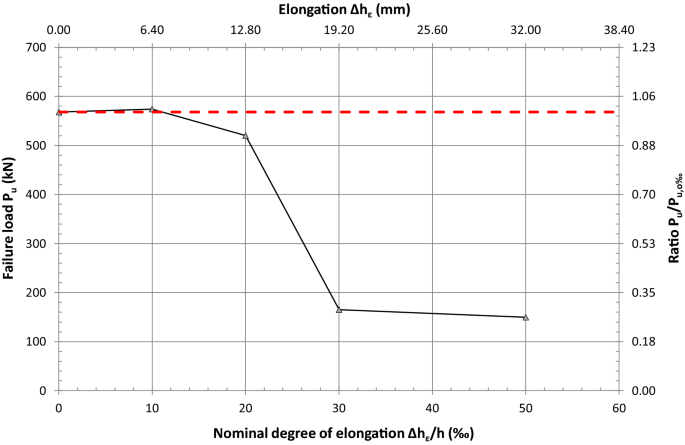
Change of ultimate failure load relative to the degree of elongation.
Fig. 11 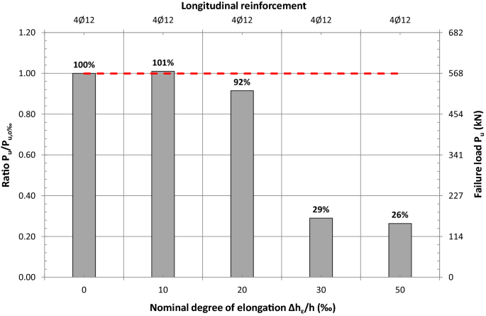
Column diagram of ultimate failure load as a percentage of the failure load of the “initial” specimen regarding the degree of elongation.
Table 4 Maximum failure load during the compression test. - 2.
As far as the formation of cracks and the mode of failure are concerned, it is noted that the crack formation and the behavior of specimens were different according to the pre-tensile degree they have sustained. First of all, test element C-0, since it was subjected only to compression load, no tensile cracks were formed and the specimen failed due to the excess of its compressive load capacity. For prisms with low degrees of elongation (specimens C-10 and C-20), it is evident that the tensile cracks formed during the first loading cycle (tensile cycle), they close when specimens are strained under compression load at the second loading cycle (compression cycle) (Figs. 4, 5). Thus, failure stems from the excess of the load bearing capacity of those specimens in compression. Small buckling phenomena make their presence at the beginning of the compression cycle, but when the cracks close because of the compression strain applied, these bubkling phenomena gradually disappear and the specimens return to their initial (non-buckled) state. For elements with high degrees of elongation (specimens C-30 and C-50), it is apparent that the tensile cracks formed during the first tensile loading cycle have such large widths, due to the large values of tensile strains applied (Fig. 4), that make it impossible to close when compression is applied at the second loading cycle. Thus, cracks are unable to be closed and remain open and significant buckling phenomena appear when compression load is applied. Both specimens with high elongation degrees fail because of buckling around their weak axis (Fig. 5). Table 5 displays the different types of failure for each specimen. It is obvious that specimens with no tensile degree (C-0) or low tensile degree (C10, C-20) fail due to an excess of the cross-sectional load bearing capacity in compression, while specimens strained with high elongation degrees (C30, C-50) fail clearly due to buckling.
Table 5 Types of failure of specimens at the end of compression test. - 3.
The vertical deformation (shortening) of the columns at the point of the ultimate failure load is influenced by the degree of elongation applied on specimens during the first tensile cycle of loading. Table 6 displays axial deformations at the point of critical failure load for all five specimens. For elongation degree 0‰, shortening at the point of failure is equal to 4.53‰ (2.90 mm). For degree of elongation 10‰, axial deformation for ultimate failure load increases and becomes equal to 17.19‰ (11.00 mm). This is logical because for low-degree specimens, cracks close and then the compressive resistance of the specimen is developed, till its excess, leading to prism failure. This means that the shortening imposed during the second compression loading cycle is bigger than the tensile strain applied at the first tensile loading cycle. Thus, for specimen C-10, tensile strain applied is equal to 10‰, and then at the compression cycle the shortening applied till failure exceeds the value of 10‰ and gets a value equal to 17.19‰. The same phenomenon appears for element C-20. Cracks again close before specimen C-20 develops its compression resistance, till its excess, leading to prism failure. In that case, the axial deformation needed for the test specimen to fail is again larger than the tensile strain applied at the first loading cycle (20‰) and is equal to 24.44‰. For elongation degrees equal to 30‰ and 50‰, axial deformation remains the same and at both cases equal to 4.69‰. It is apparent that in the cases of specimens suffering a high tensile degree (C30, C-50), the shortening of the columns for maximum failure load is not larger than the elongation of the columns at the first cycle of loading. Furthermore, the axial deformation at failure (4.69‰) is much smaller than tensile strain applied (30‰ and 50‰). This can be explained since high-degree prisms fail due to buckling and not because of the excess of their cross-sectional compressive strength. That means that cracks do not close before failure and the compression strength is not developed. Since cracks remain open till failure, that means that the shortening at failure is much smaller than the elongation subjected to the tensile cycle. Figure 12 shows the values of axial deformation at the point that failure takes place, meaning for the critical failure load.
Table 6 Axial deformations for maximum failure load of compression test. Fig. 12 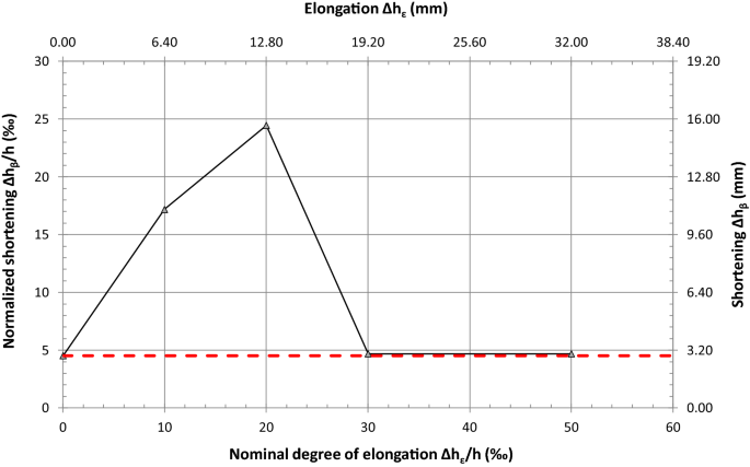
Variation of shortening at failure versus the degree of elongation.
- 4.
Table 6 presents also the value of the actual normalized shortening needed for the specimen to fail. For specimen C-0, the actual normalized shortening is equal to the value measured, since this specimen suffered no tensile strain. As far as elements C-10 and C-20 are concerned, the actual normalized shortening is calculated by subtracting the value measured from the value of the tensile elongation that each specimen suffered, since the cracks for these two specimens close and the columns return to their initial (non-deformed) state and from that point the compression strength of specimen is developed, till its excess, that leads to failure. E.g. the value equal to 7.19‰ for element C-10 is calculated as 17.19‰ − 10‰ = 7.19‰. For column C-20, the value equal to 4.44‰ is estimated as 24.44‰ − 20‰ = 4.44‰. For specimens strained under high degrees of elongation (C30, C-50), the normalized shortening measured for ultimate failure load is the actual normalized shortening needed for the specimens to fail. This is because these two specimens do not return to their initial (non-deformed) shape, the cracks never close and the specimens fail due to buckling. Thus, the measured value of axial deformation is the actual value needed for the specimens to fail. It can be easily noticed that in all cases of all five specimens, the value of normalized axial deformation needed for the specimens to fail is of the order of about 5‰. Further tests need to be conducted on this matter before a more reliable answer can be given.


4 Analytical Procedure
4.1 Empirical Equation for Ultimate Failure Load
There has been effort to correlate analytically the ultimate failure load of specimens with the degree of elongation that have sustained. Figure 11 makes it obvious that critical failure load is expressed as a percentage of the maximum load of the “initial” specimen. Through IBM SPSS Statistics v25.0, a non-linear regression analysis was conducted to isolate an equation that could correlate the ultimate failure load with elongation degree (for each specimen). The model derived has taken the following form:
where Pu is the specimen’s ultimate failure load; α–δ are the coefficients resulted by the regression analysis; ε is the tensile degree each specimen has been subjected to; in values per mille; Pu,o is the ultimate load of failure of the “initial” specimen.
Since the number of specimens tested is not enough for the proper calibration of Eq. (1), results from experiments found in the international literature are used. These experiments have taken place on specimens modeling the confined boundaries of reinforced concrete walls again, but using different longitudinal reinforcement ratios. Table 7 gives a summary of the test data of the specimens found in the international study performed by the same author (Chrysanidis 2019) and used herein for the better calibration of Eq. (1). Various values for elongation degrees were used. The specimens used for comparison purposes were strained under uniaxial loading, too. A specimen is used for comparison purposes at this study, too, and this specimen is characterized as reference or control specimen. It serves the same purpose like the “initial” specimen used in the current study.
Thus, using the elements of the current study and the specimens of bibliography given at Table 7, Eq. (1) takes the following form:
It is obvious that the values of the constants α–δ of Eq. (2) have taken a somewhat different value compared to the values of the same parameters α–δ, calculated by the same author in a previous research (Chrysanidis 2019). Correlation coefficient R2 for Eq. (2) was found by the software to be equal to 0.978. Table 8 compares the experimental with the analytical values, but only for the five specimens of the current research. Figure 13 depicts the data given in Table 8 in the form of a plot. It is obvious, both from Table 8 and Fig. 13, that the calibrated Eq. (2) using 15 specimens in total (5 tested herein and 10 found in international bibliography) gives a good correlation for the five specimens of the current work. The comparison of the experimental values to the empirical ones using their ratio (Table 8) proves that the correlation between the two types of values is good, except for the two last values corresponding to specimens strained under degrees of elongation equal to 30‰ and 50‰—even for the last two values the correlation can be characterized as satisfactory.

Comparison of experimental and analytical diagrams of ultimate failure load against compressive loading for specimens of the current work.
Figure 14 displays the correlation between the analytically calculated values and the ones resulted from the compressive tests of the second stage of loading using the five columns belonging to the present study and the 10 prisms taken from another study of the same author (Chrysanidis 2019). It is noticed that almost all specimens found in bibliography fall inside the dashed lines representing a field of ± 20% difference from the middle continuous line of absolute correlation. Only two specimens fall a little higher from the dashed line representing + 20% difference to the absolute correlation given from the continuous line and two other specimens fall a little bit lower below the line of − 20% difference. Thus, this means that in total there are four specimens outside of the region that the two dashed lines define. This fact proves the good accuracy of Eq. (2) to predict the maximum failure loads for specimens strained under different degrees of elongation. The comparison between the experimental and the analytical failure loads for the 10 specimens of bibliography, along with the name of each specimen, are given at Table 9.

Cross-plot of experimental values of ultimate failure load versus analytical values found from the regression Eq. (2) for specimens of the current research and specimens found in the bibliography.
4.2 Empirical Equation for Shortening at Maximum Failure Load
Using again the same software IBM SPSS Statistics v25.0, a correlation takes place between the normalized axial compressive deformation at the point of failure and the degree of pre-tensile strain that the specimens have been subjected to, along with the axial displacement of the “initial” specimen. Thus, the model in question has the form of the following equation:
where Δhβ,Pu is the specimen’s shortening for the ultimate failure load; in values per mille; α–δ are the coefficients resulted by the regression analysis; ε is the tensile degree each specimen has been subjected to; in values per mille; Δhβo,Puo is the “initial” specimen’s shortening for the failure load; in values per mille.
Since the number of specimens tested is not enough for the proper calibration of Eq. (3), results from experiments found in the international literature are used, once again. The characteristics of the test specimens found in the literature have been given at Table 7 (Chrysanidis 2019) and used herein for the better calibration of Eq. (3).
Thus, using the elements of the current study and the specimens of bibliography given at Table 7, Eq. (3) takes the following form:
Correlation coefficient R2 for Eq. (4) was found by the software to be equal to 0.919. Table 10 compares the experimental with the analytical values, but only for the five specimens of the current research. Figure 15 depicts the data given in Table 10 in the form of a plot. It is obvious, both from Table 10 and Fig. 15, that the calibrated Eq. (4) using 15 specimens in total (5 tested herein and 10 found in international bibliography) gives a good correlation for the five specimens of the current work. The comparison of the experimental values to the empirical ones using their ratio (Table 10) proves that the correlation between the two types of values is good, except for the two last values corresponding to specimens strained under degrees of elongation equal to 30‰ and 50‰—especially for the specimen C-30.

Comparison of experimental and analytical diagrams of normalized shortening at failure for specimens of the current work.
Figure 16 displays the correlation between the analytically calculated values and the ones resulted from the compressive tests of the second stage of loading using the five columns belonging to the present study and the 10 prisms taken from another study of the same author (Chrysanidis 2019). It is noticed that almost all specimens found in bibliography fall inside the dashed lines representing a field of ± 20% difference from the middle continuous line of absolute correlation. Only one specimen falls much higher from the dashed line representing + 20% difference and only one specimen falls a little bit higher from the same dashed line. Two other specimens fall a little bit lower below the line of − 20% difference. Thus, this means that in total there are four specimens outside of the region that the two dashed lines define. This fact proves the good accuracy of Eq. (4) to predict the normalized shortening at failure for specimens strained under different degrees of elongation. The comparison between the experimental and the analytical failure loads for the 10 specimens of bibliography, along with the name of each specimen, are given at Table 11.

Cross-plot of experimental values of normalized shortening for ultimate failure load versus analytical values found from the regression Eq. (4) for specimens of the current research and specimens found in the bibliography.
5 Conclusions
In this paper, five reinforced concrete column test specimens simulating the confined boundaries of seismic walls were tested to evaluate the structural performance in terms of the damage process, mode of failure and ultimate bearing load. All prisms were strained under varying extents of tensile degradation and then put through uniaxial compressive load. For the comparison, one “initial” element was manufactured and strained only to compression load. As per the results, these conclusions come forth:
- 1.
Degree of tensile deformation plays a substantial part in the damage process, failure mode and maximum bearing capacity of walls. It affects tremendously all the previous characteristics of the extreme edges of shear walls.
- 2.
After a certain value of elongation degree, failure mode changes from concrete crushing to buckling. At the same time, critical failure load sustains a significant drop compared to specimens strained to lower tensile degrees. It is obvious that the increase, after a certain value, of the degree of tensile strain results to a significant decrease of the ultimate bearing capacity of confined boundaries and it should be taken into account when designing structural walls.
- 3.
After this critical elongation degree, damage process changes when specimens are subjected to compressive load. Cracks remain open, especially to the tensile side of the prisms. In contrast, cracks for lower degrees of elongation eventually close, leading to the development of the section’s compressive capacity.
- 4.
Design of structural walls and calculation of their thickness according to modern seismic and concrete codes should take into account the degree of elongation apart from the bottom storey height. This is necessary since it has been shown in the present study that tensile elongation affects load-carrying capacity against compressive loading for the extreme boundaries of reinforced concrete walls.
- 5.
It seems that even walls reinforced at their confined boundaries with the maximum allowable longitudinal reinforcement ratio by modern seismic and concrete codes cannot inhibit lateral buckling failure after a certain degree of tensile deformation. Further work is needed on the subject to look at the impact of the mechanical factor of reinforcement ratio. Nevertheless, it is noteworthy that the detailing of extreme edges with the usage of the maximum longitudinal reinforcement ratio does not halt the phenomenon of transverse instability.
- 6.
Actual value of axial compressive deformation at the moment of failure, basically, remains in the same order, independent of the tensile strain applied during the tensile loading cycle. This fact shows that the actual compressive strain, need to be applied before failure of specimens is reached, stays indifferent and is not affected by the degree of elongation that the specimens have sustained.
Availability of data and materials
The datasets used and/or analysed during the current study are available from the corresponding author on reasonable request.
References
Adebar, P., Ibrahim, A. M. M., & Bryson, M. (2007). Test of high-rise core wall: Effective stiffness for seismic analysis. ACI Structural Journal, 104(5), 549–559.
Almeida, J., et al. (2017). Tests on thin reinforced concrete walls subjected to in-plane and out-of-plane cyclic loading. Earthquake Spectra, 33(1), 323–345. https://doi.org/10.1193/101915EQS154DP.
Bendito, A., et al. (2009). Inelastic effective length factor of nonsway reinforced concrete columns. Journal of Structural Engineering, 135(9), 1034–1039. https://doi.org/10.1061/(asce)0733-9445(2009)135:9(1034).
Bertero, V. V. (1980). Seismic behavior of R/C wall structural systems. In 7th world conference on earthquake engineering (pp. 323–330).
Beyer, K. (2015). Future directions for reinforced concrete wall buildings in Eurocode 8. In SECED 2015 conference: Earthquake risk and engineering towards a Resilient World, August (pp. 1–7).
Canadian Standards Association. (2007). CAN, CSA-A23.3-04, design of concrete structures (update no. 2—July 2007). Mississauga, Ontario, Canada: Canadian Standards Association.
Chai, Y. H., & Elayer, D. T. (1999). Lateral stability of reinforced concrete columns under axial reversed cyclic tension and compression. ACI Structural Journal, 96(5), 780–789.
Chai, Y. H., & Kunnath, S. K. (2005). Minimum thickness for ductile RC structural walls. Engineering Structures, 27(7), 1052–1063. https://doi.org/10.1016/j.engstruct.2005.02.004.
Chrysanidis, T. (2019). Influence of elongation degree on transverse buckling of confined boundary regions of R/C seismic walls. Construction and Building Materials, 211, 703–720. https://doi.org/10.1016/J.CONBUILDMAT.2019.03.271.
Elnashai, A. S., Pilakoutas, K., & Ambraseys, N. N. (1990). Experimental behaviour of reinforced concrete walls under earthquake loading. Earthquake Engineering and Structural Dynamics, 19(3), 389–407. https://doi.org/10.1002/eqe.4290190308.
Elwood, K. J., & Eberhard, M. O. (2009). Effective stiffness of reinforced concrete columns. ACI Structural Journal, 106(4), 476–484.
European Committee for Standardization. (2004a). EN 1992-1-1:2004, Eurocode 2: Design of concrete structures—Part 1-1: General rules and rules for buildings. Belgium, Brussels: European Committee for Standardization.
European Committee for Standardization. (2004b). EN 1998-1:2004, Eurocode 8: Design of structures for earthquake resistance—Part 1: General rules, seismic actions and rules for buildings. Belgium, Brussels: European Committee for Standardization.
Farrar, C. R., & Baker, W. E. (1993). Experimental assessment of low-aspect-ratio, reinforced concrete shear wall stiffness. Earthquake Engineering and Structural Dynamics, 22(5), 373–387. https://doi.org/10.1002/eqe.4290220502.
Fintel, M. (1991). Shear walls—an answer for seismic resistance? Concrete International, 13(7), 48–53.
Fintel, M. (2014). Performance of buildings with shear walls in earthquakes of the last thirty years. PCI Journal. https://doi.org/10.15554/pcij.05011995.62.80.
Gould, N. C., & Harmon, T. G. (2002). Confined concrete columns subjected to axial load, cyclic shear, and cyclic flexure—Part II: Experimental program. ACI Structural Journal, 99(1), 42–50.
Gran, J. K., & Senseny, P. E. (2002). Compression bending of scale-model reinforced-concrete walls. Journal of Engineering Mechanics, 122(7), 660–668. https://doi.org/10.1061/(asce)0733-9399(1996)122:7(660).
Ho, J. C. M., & Pam, H. J. (2003). Inelastic design of low-axially loaded high-strength reinforced concrete columns. Engineering Structures, 25(8), 1083–1096. https://doi.org/10.1016/S0141-0296(03)00050-6.
International Conference of Building Officials. (1997). Uniform building code—volume 2: Structural engineering design provisions. Whittier, California, USA: International Conference of Building Officials.
Kassem, W., & Elsheikh, A. (2010). Estimation of shear strength of structural shear walls. Journal of Structural Engineering, 136(10), 1215–1224. https://doi.org/10.1061/(asce)st.1943-541x.0000218.
Lee, H. S., & Ko, D. W. (2007). Seismic response characteristics of high-rise RC wall buildings having different irregularities in lower stories. Engineering Structures, 29(11), 3149–3167. https://doi.org/10.1016/j.engstruct.2007.02.014.
Li, Q. S. (2001). Stability of tall buildings with shear-wall structures. Engineering Structures, 23(9), 1177–1185. https://doi.org/10.1016/S0141-0296(00)00122-X.
Lu, Y., et al. (1999). Reinforced concrete scaled columns under cyclic actions. Soil Dynamics and Earthquake Engineering, 18(2), 151–167. https://doi.org/10.1016/S0267-7261(98)00037-2.
Mazars, J., Kotronis, P., & Davenne, L. (2002). A new modelling strategy for the behavior of shear walls under dynamic loading. Earthquake Engineering and Structural Dynamics, 31(4), 937–954. https://doi.org/10.1002/eqe.131.
Ministry of Environment Planning and Public Works. (2000). Greek code for the design and construction of concrete works, Athens, Greece (In Greek).
Mo, Y. L., Zhong, J., & Hsu, T. T. C. (2008). Seismic simulation of RC wall-type structures. Engineering Structures, 30(11), 3167–3175. https://doi.org/10.1016/j.engstruct.2008.04.033.
Moyer, M. J., & Kowalsky, M. J. (2003). Influence of tension strain on buckling of reinforcement in concrete columns. ACI Structural Journal, 100(1), 75–85.
Orakcal, K., Wallace, J. W., & Conte, J. P. (2014). Flexural modeling of reinforced concrete walls-model attributes. ACI Structural Journal, 101(5), 688–698. https://doi.org/10.14359/13391.
Parra, P. F., & Moehle, J. P. (2014). Lateral buckling in reinforced concrete walls. In Tenth U.S. national conference on earthquake engineering.
Paulay, T., & Priestley, M. J. N. (1993). Stability of ductile structural walls. ACI Structural Journal, 90(4), 385–392.
Penelis, G. G., & Kappos, A. J. (1996). Earthquake-resistant concrete structures. London: Chapman & Hall.
Penelis, G., et al. (1995). Reinforced concrete structures. Thessaloniki, Greece: A.U.Th. Press.
Pessiki, S., & Pieroni, A. (1997). Axial load behavior of large-scale spirally-reinforced high-strength concrete columns. ACI Structural Journal, 94(3), 304–314.
Pilakoutas, K., & Elnashai, A. (1995). Cyclic behavior of reinforced concrete cantilever walls, Part I: Experimental results. ACI Structural Journal, 92(3), 271–281.
Rad, B. R., & Adebar, P. (2009). Seismic design of high-rise concrete walls: Reverse shear due to diaphragms below flexural hinge. Journal of Structural Engineering, 135(8), 916–924. https://doi.org/10.1061/(asce)0733-9445(2009)135:8(916).
Raju, R. (2017). Behaviour of corner beam column joint with rectangular spiral reinforcement and longitudinal FRP bars. International Research Journal of Advanced Engineering and Science, 2(2), 160–165.
Rosso, A., Almeida, J. P., & Beyer, K. (2016a). Out-of-plane behaviour of reinforced concrete members with single reinforcement layer subjected to cyclic axial loading: Beam-column element simulation. In Proc. of the 2016 NZSEE conference.
Rosso, A., Almeida, J. P., & Beyer, K. (2016b). Stability of thin reinforced concrete walls under cyclic loads: State-of-the-art and new experimental findings. Bulletin of Earthquake Engineering, 14(2), 455–484. https://doi.org/10.1007/s10518-015-9827-x.
Rosso, A., et al. (2018). Cyclic tensile-compressive tests on thin concrete boundary elements with a single layer of reinforcement prone to out-of-plane instability. Bulletin of Earthquake Engineering, 16(2), 859–887. https://doi.org/10.1007/s10518-017-0228-1.
Rosso, A., et al. (2017). Experimental campaign on thin RC columns prone to out-of-plane instability: Numerical simulation using shell element models. In VIII Congreso Nacional de Ingeniería Sísmica.
Rosso, A., et al. (2016). Experimental tests on the out-of-plane response of RC columns subjected to cyclic tensile-compressive loading. In 16th world conference on earthquake engineering.
Sheikh, S., & Khoury, S. (1993). Confined concrete columns with stubs. ACI Structural Journal, 90(4), 414–431.
Stability, B. R., & Walls, S. R. C. (2019). Assessment of the Boundary region stability of special RC walls | SpringerLink Page 1 of 3 assessment of the boundary region stability of special RC walls assessment of the boundary region stability of special RC walls | SpringerLink Page 2 of 3 Personali. vol. 1, pp. 13–15.
Standards New Zealand. (2006). NZS 3101:2006, concrete structures standard: Part 1—the design of concrete structures,. Wellington, New Zealand: Standards New Zealand.
Taleb, R., Tani, M., & Kono, S. (2016). Performance of confined boundary regions of RC walls under cyclic reversal loadings. Journal of Advanced Concrete Technology, 14(4), 108–124. https://doi.org/10.3151/jact.14.108.
Tan, T. H., & Yip, W. K. (1999). Behavior of axially loaded concrete columns confined by elliptical hoops. ACI Structural Journal, 96(6), 967–971.
Taylor, C., & Wallace, J. (1995). Design of slender reinforced concrete walls with openings. Report No. CU/CEE-95/13, Department of Civil and Environmental Engineering, Clarkson University, Potsdam, New York.
Wallace, J. W. (2010). Performance-based design of tall reinforced concrete core wall buildings. Geotechnical, Geological and Earthquake Engineering, 17, 279–307. https://doi.org/10.1007/978-90-481-9544-2_12.
Wallace, J. W. (2012). Behavior, design, and modeling of structural walls and coupling beams—lessons from recent laboratory tests and earthquakes. International Journal of Concrete Structures and Materials, 6(1), 3–18. https://doi.org/10.1007/s40069-012-0001-4.
Wallace, J. W., & Moehle, J. P. (2007). Ductility and detailing requirements of bearing wall buildings. Journal of Structural Engineering, 118(6), 1625–1644. https://doi.org/10.1061/(asce)0733-9445(1992)118:6(1625).
Wood, S. L., Wight, J. K., & Moehle, J. P. (1987). The 1985 Chile earthquake: Observations on earthquake resistant construction in Viña del Mar. ReportNo. UILU-ENG-87-2002, Department of Civil Engineering, University of Illinois at Urbana-Champaign, Urbana, Illinois.
Zhang, Y., & Wang, Z. (2001). Seismic behavior of reinforced concrete shear walls subjected to high axial loading. Structural Journal, 97, 739–750.
Acknowledgements
Not applicable.
Funding
Not applicable.
Author information
Authors and Affiliations
Contributions
There is only one author in the current study. Thus, the whole experimental and analytical work presented has been carried out by the only author. The author read and approved the final manuscript.
Corresponding author
Ethics declarations
Competing interests
The author declares no competing interests.
Additional information
Publisher's Note
Springer Nature remains neutral with regard to jurisdictional claims in published maps and institutional affiliations.
Journal information: ISSN 1976-0485 / eISSN 2234-1315
Rights and permissions
Open Access This article is licensed under a Creative Commons Attribution 4.0 International License, which permits use, sharing, adaptation, distribution and reproduction in any medium or format, as long as you give appropriate credit to the original author(s) and the source, provide a link to the Creative Commons licence, and indicate if changes were made. The images or other third party material in this article are included in the article's Creative Commons licence, unless indicated otherwise in a credit line to the material. If material is not included in the article's Creative Commons licence and your intended use is not permitted by statutory regulation or exceeds the permitted use, you will need to obtain permission directly from the copyright holder. To view a copy of this licence, visit http://creativecommons.org/licenses/by/4.0/.
About this article

Cite this article
Chrysanidis, T.A. Evaluation of Out-of-Plane Response of R/C Structural Wall Boundary Edges Detailed with Maximum Code-Prescribed Longitudinal Reinforcement Ratio. Int J Concr Struct Mater 14, 3 (2020). https://doi.org/10.1186/s40069-019-0378-4
Received:
Accepted:
Published:
DOI: https://doi.org/10.1186/s40069-019-0378-4