Abstract
The dispersion relations for bulk and surface plasmon-polaritons in a semi-infinite 1D photonic crystal interlayered with graphene are calculated in the presence of an applied magnetic field. The results are applied to SiO2 as the constituent material in geometry where the layers are arranged in a periodic array with the same layer thickness. The static magnetic field is applied perpendicular to the plane of layers. Numerical results are presented for the modes in THz range, up to 10 THz, to illustrate the important role of the applied magnetic field on the graphene sheets in modifying the polariton dispersion curves, especially for magnetic fields of the order of 1 T. It is found that the polariton frequencies and band gaps have a sensitive dependence on the electron scattering rate parameter (and hence the applied magnetic field strength) in the graphene sheets. Electromagnetic retardation effects are fully taken into account for the bulk bands, while for the surface modes (which are shown to have a novel non-reciprocal propagation characteristics) it is convenient to focus on the regime where retardation is small.
Export citation and abstract BibTeX RIS
1. Introduction
One-dimensional (1D) graphene photonic crystals (PCs) are multilayered systems where one of the constituent materials is graphene, the well-known one-atom-thick metallic film discovered in 2004 [1]. These graphene PCs form an emergent research area of intense interest [2–8]. Systems such as PCs [9] or quasicrystals [10] that incorporate the atomically-thin graphene material have been studied because they exhibit novel optical properties and may be valuable for modern applications in the field of tunable plasmonic and graphene electronics at far-infrared frequencies, for example. Also, these structures can support highly confined plasmon polaritons with very low loss [11] due to graphene's unique electronic dispersion with gapless features near the so-called Dirac points in the Brillouin zone [12].
Polaritons are hybrid (or mixed) modes that occur when a photon strongly couples to an excitation in the material [13, 14]. Examples include exciton-polaritons, when a photon couples to an electron–hole pair in a semiconductor, or plasmon-polaritons, when the coupling is with the electron plasma in a metal or doped semiconductor. On the other hand, graphene constitutes a very special kind of 2D electron gas system. For example, the capability to change its carrier concentration using an applied voltage-gate opens the way to precise control of the frequency range for excitations like surface plasmon-polaritons (SPP) [15]. Also long propagation lengths can be achieved [16] compared with conventional SPPs.
On the other hand, it is known that when an external magnetic field is applied perpendicular to a 2D electron gas [16] a mix between cyclotron excitations and the electronic oscillations (or plasmons) occurs in that system, leading to magnetoplasmon-polaritons [17]. An effect of the magnetic field is to cause an anisotropy in the optical conductivity tensor and strong resonant absorptions in the dielectric functions. Consequently the dispersion properties and frequencies of the polaritons become very sensitive to the applied magnetic field, especially in systems that incorporate graphene sheets [18–20]. For example, Ferreira et al [19] reported an exotic polariton mode with weak damping in a single-layer graphene film with an applied static magnetic field; they termed it a quasi-transverse-electric mode because of the resemblance to conventional transverse electric (TE) modes. Also Melo [21] studied the excitation of surface polaritons in magnetically biased graphene at the interface separating two dielectric media. The focus was on the influence of the magnetostatic field for the surface polaritons in graphene in the 500 GHz to 5 THz frequency range, where the author calculated the reflectance in an attenuated total reflection (ATR) set up [14] and associated the reflectance dip with the excitation of the surface polaritons. Michalski [22] used the modal transmission line theory to calculate the reflectivity and transmissivity rate in a multilayered system with multiple anisotropic conductive graphene sheets at the interfaces. He noted that the analysis of such structures is rendered non-trivial, because of the coupling between the transverse magnetic (TM) and TE polarization field caused by the graphene sheets. It was concluded that a TE plane wave should also excite SPP modes, due to this coupling of the TE and TM waves, and this coupling becomes enhanced with increased magnetic field bias.
In this work we emphasize the role (and its interesting consequences) of an applied magnetic field on the surface and bulk plasmon-polariton modes in a photonic crystal with embedded graphene sheets at the interfaces, henceforth referred to as a graphene photonic crystal (GPC). The plasmon-polaritons are studied here by using Maxwell's equations in a macroscopic formalism, where graphene is characterized by a frequency-dependent optical conductivity tensor. In section 2 we present a modification of the plasmon-polariton theory for dielectric photonic crystal with graphene sheets [9] to relate to our present case where we have an external magnetic field applied. Here the graphene sheets are characterized by a modified optical conductivity, which includes the Landau levels' quantization due to the applied magnetic field, and we concentrate initially on the bulk polaritons. Next the localized surface polaritons of a semi-infinite GPC are considered in section 3. Numerical results are then presented in section 4 when the dielectric material is taken to be SiO2 in the various layers of the GPC. These results illustrate the important role of the applied magnetic field in GPCs in modifying the polariton dispersion curves, especially when we have a magnetic field of order 1 T. Also we report a sensitive dependence on the polariton dispersion relation curves on the electronic scattering rate parameter and on the intensity of the applied magnetic field in the graphene sheets. In the last section we present the conclusions of this work.
2. General theory
We consider a photonic crystal (PC) consisting of alternating unit cells AB juxtaposed to form the periodic ABABAB... array, with graphene sheets at each of the interfaces and a static magnetic field  applied in the direction perpendicular to the layers (see figure 1). The building blocks A and B are layers of a dielectric material with thicknesses a and b, respectively.

Figure 1. The geometry and coordinate axes for the 1D PC array (ABABAB...) with graphene sheets at each of the interfaces. In the case of a semi-infinite array with a surface at z = 0 the external medium is denoted as C.
Download figure:
Standard image High-resolution image2.1. Field-dependent conductivity of graphene
When a static magnetic field B0 is applied perpendicular to the graphene sheets, it is known that the conductivity becomes a tensor with the components in the xy-plane satisfying [23]
Here, the general expressions for the diagonal and off-diagonal terms (sometimes called Hall conductivities) can be obtained using the Kubo formula [18, 24] as
The summations over n are for the energies  of the Landau level, nF is the Fermi–Dirac distribution function at temperature T,
  is the Fermi velocity of the electrons in graphene,
  is the electron scattering rate,
  sgn(B0) is the sign function of
  , and e is the electron charge. Here we have considered the excitonic energy to be equal to zero, i.e.
  in [24].
When  , the sums over n for
  go to zero and
  converges very slowly. In this case (not studied here) we could alternatively use the Drude form given in [21, 25]. To illustrate the behaviour of the optical conductivity for graphene for the field values of interest, we consider T = 300 K, chemical potential
  eV for the graphene sheets [26–28], and electron scattering rate
  meV [21]. Figure 2 shows
  and
and  plotted versus frequency for the values of the applied magnetic field, B0 = 0.5, 1.0, and 1.5 T, where the solid (dashed) lines correspond to the real (imaginary) part of
  (in figure 2(a)) and
  (in figure 2(b)). The vertical lines (located at the frequencies 0.390 and 0.558 THz) characterize the maximum and minimum value for the imaginary part of
  (real part of
  ), respectively, when B0 = 1.5 T. These values will turn out to be important later for interpreting the bulk polariton dispersion relations.
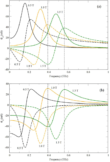
Figure 2. The diagonal,  (a), and off-diagonal,
  (b), components of the graphene conductivity tensor as functions of the frequency for several values of the applied magnetic field B0. The solid (dashed) lines are the real (imaginary) part of
  and
and  . The vertical lines are explained in the text.
Download figure:
Standard image High-resolution image2.2. Bulk polariton modes
In order to study the bulk polariton modes for an infinite GPC, we need to consider solutions of Maxwell's equations within each dielectric medium, subject to the standard electromagnetic boundary conditions at the interfaces with graphene. As a consequence of the Landau levels leading to a non-diagonal conductivity tensor for the graphene sheets, we need to consider the electric and magnetic field solutions within the constituent media A and B of the lth layer in a general way. Specifically, we do not make a separation into particular polarizations like TM or TE. Instead, in both media we write  for the electric fields, where


The factors  ,
,  ,
,  , and
, and  (with j = A or B;
  ) are the amplitudes for the forward- and backward-travelling waves, respectively, and L = a + b is the periodicity length. Without loss of generality, we have taken the in-plane wave vector to be along the x direction, and so
  for the (complex) wave vector in the perpendicular direction.
Correspondingly, for the magnetic field components  in medium A (or B), we deduce from
  that
that

From the electromagnetic boundary conditions at any A − B interface we require


Then, by considering these condition at the interfaces z = nL + a within a cell and at  between cells (see figure 1), we can relate the electromagnetic fields for cell n to those for cell n + 1. From equation (10) we deduce


Next from equations (11) and (12) we can write
where we define  ,
,  ,
,  , and
, and  . The above equations can be conveniently re-expressed in a matrix form as
Here the  propagation matrix MA is simply given by
while the more complicated  interface matrix due to the graphene sheet is defined in block form as
where the forms of the  matrices
  (with
(with  and
and  taking the values 1 or 2) are specified in the appendix.
An analogous matrix equation arises when we apply the same boundary conditions at the interfaces where  . In this case it relates the amplitudes
  and
and  (
( ) to
) to  and
and  , giving
Here MB and MBA are the same as MA and MAB, respectively, provided the substitutions  ,
,  , and
, and  in the matrices (19) and (18) are made. On defining the kets formed by the undetermined set of coefficients as
we find that equations (17) and (20) can be re-expressed as the matrix equations


It is easy to show that, using these equations, we obtain

where in the last step Bloch's theorem (see [14]) was employed, with Q being the modulus of the Bloch wave vector. Here the so-called transfer matrix T is given by

and therefore

where I is the  unit matrix. The equation above is the secular equation that defines the bulk polariton dispersion relation. From the property that T is an unimodular matrix (det T = 1) it can be shown [29] that its eigenvalues
  occur in reciprocal pairs, allowing us to write
  and
and  . Therefore, as we conclude below, it is necessary only to find two eigenvalues, which are related to the Bloch wave vectors through [29]

By solving equation (26) we find that the eigenvalues satisfy the polynomial equation  , where the coefficients are related to the elements of the transfer matrix by

After some straightforward algebra the above polynomial can be rearranged as

with  . This roots of this equation, together equation (24), gives us the dispersion relations for the bulk bands in the form

where
In this case we have two independent solutions for the Bloch wave vector Qi, as illustrated later by numerical examples.
It is worth noting that, as a special case of the above theory, we may use equation (17) to consider the polaritons propagating at a single interface (at z = a) between two different semi-infinite media (A and B). The general result reduces to
which leads to a  matrix secular equation for the polariton modes. After some algebra, we can recover the result given in [19] for the single graphene sheet at the interface between two media, i.e.
where we define  and
and  .
.
3. Surface polariton modes
For a study of the surface modes we consider a semi-infinite GPC with the geometry as in figure 1, where the region z < 0 is taken to be a dielectric medium C. In practice, a surface mode in a photonic crystal is excited by an incident electromagnetic wave either in p-polarization (a TM mode) or s-polarization (a TE mode), e.g. as in an ATR experiment. Here we will consider both the cases of p-polarization and s-polarization in the external medium C.
3.1. Case of p-polarization in the external medium
We consider now a p-polarized wave incident on the PC sample from the external medium C. The electric and magnetic fields are given by  and
and  , where

Here,  and we assume
  so that kzC takes only real and positive values. To obtain equations (36) and (37), we used
  together with
  . By applying the previous electromagnetic boundary conditions as in equations (10)–(12) to the interface at z = 0, we have


From these coupled equation we can deduce a relationship between the  and
and  amplitudes. The result is

where

Then from equations (40)–(42) we can write

where
For the semi-infinite GPC in figure 1, instead of using Bloch's theorem as in the bulk-mode case, we now seek solutions for localized SPP that have decaying amplitudes for the electromagnetic fields with respect to distance from one unit cell to the next interior cell, starting from the surface plane z = 0. Therefore, taking equation (24) with  , we must have

with Re (or equivalently
  ) as a requirement for localization. On applying this equation to the first layer, we have (following [13])
From this equation, we can find two conditions for localized surface modes. One condition comes from writing out the first and second lines of equation (47) in full, and leads to

together the condition

Also, from the third and fourth lines of (47), we obtain a second implicit dispersion relation for surface modes as

together with

Two brief comments on the above results are useful. First, if we put  , we just recover the polariton results in our previous paper [9] where there was no applied magnetic field. Secondly, our present results for the surface modes simplify in the regime where retardation effects are small (as at larger in-plane wavenumbers). In this case, choosing
  and
and  , following [30], the parameters in equations (43) and (45) reduce to
3.2. Case of s-polarization in the external medium
To obtain the surface modes in a semi-infinite GPC in the case of an incident wave with s-polarization (TE) we write  and
and  , where

To obtain equations (55) and (56) we used 
 . Now, by applying the same boundary conditions, (10)–(12), we have


for the electrical fields amplitudes, and
for the magnetic fields amplitudes. In similar way as for p-polarization, we have from (57),  . Therefore, applying it in (59) and (60) we have
Now, using (58), we can rewrite (3.2) as
After some algebra we can find

or
with
By using (57) and (58) we can find
and
with
The conditions for having localized s-polarized surfaces modes can be obtained using the transfer matrix in a similar fashion to the analysis in the previous subsection for the case of p-polarization. The analogous equations to (48)–(51) are found to be


with the localization conditions


Again there are simplifications in the case of weak retardation. Specifically, equations (66) and (69) reduce to give
4. Numerical results
In this section we apply the previous theory to a semi-infinite GPC to illustrate the results for the bulk and surface polaritons. We take both of the constituent materials, A and B, to be silica (SiO2), with a dielectric constant  , as appropriate for THz frequencies [31]. We mention here, as a first approximation, our results will not include the effects of absorption near 4 THz and 8 THz due to SiO2, since our goal here is to simulate a lossless material and focus on the role of the graphene layers in a magnetic field. Indeed, absorption processes will modify the properties of polaritons most sensitively when the frequencies lie close to a resonance. Generally, absorption leads to attenuation of the polaritons (surface and bulk modes) as they propagate through the crystal (see, e.g. [32]). The absorption effects could be studied in future work.
We choose vacuum ( ) for the external medium. We ignore the role of absorption on the silica since it is typically small for other distinct crystalline forms and composition [33] in the temperature and frequencies of interest in this work. Also we choose the temperature T = 300 K and a chemical potential
  eV for the graphene sheets [26–28]. The other physical parameters used here are a = b = 10
  m and applied magnetic field B0 = 1.5 T. We have put our expressions for the optical conductivity in terms of the fine structure constant
  (
( 1/137), where c is the light speed in a vacuum. This constant arises naturally from our equations. We consider the electron scattering rate (the inverse of the intrinsic relaxation time) to be
  meV [21].
In the following figures, we present numerical dispersion relations for plasmon polaritons in the 1D GPC, focusing on the effects of the applied magnetic field. The bulk modes occur here as bands separated by gaps and they are shown as the shaded areas (brown areas in the online version). These bulk bands are bounded by the curves for Qj L = 0 and  , where Qj L is given in equation (31) with L = a + b. The surface modes, characterized by black lines, lie between and above the bulk bands, subject to the constraint
  . Consequently any surface mode in these plots lies to the right of the vacuum light line (VLL), shown as a dashed straight line, given by
  . For reference, we also show the dielectric light line (DLL) for the PC given by
  . We have chosen to plot the frequency in THz units and kxa is the scaled 2D in-plane wave vector.
The bulk and surface plasmon-polariton dispersion relations for the frequency (f ) region up to 10 THz are presented in figure 3 for the in-plane wave vector ranging from kxa = −5.0 to kxa = 5.0. A reciprocal propagation effect is found for the bulk bands, as expected, with respect to the sign of the wave-vector component, but this is not the case for the surface modes where we have a non-reciprocity effect. In describing the behaviour of these modes we conveniently separate this spectrum into three distinct regions: (a) to the right (or left) side of the DLL for kx > 0 (or kx < 0) and frequencies greater than 1.0 THz; (b) inside the region bounded by the the DLLs for kx > 0 and kx < 0 with f > 1.0 THz; and (c) the region where the frequencies are less than 1 THz.

Figure 3. Polariton dispersion relation for the 1D GPC with applied magnetic field B0 = 1.5 T. Here the dashed and dotted sloping lines are the VLL and DLL, specified by  and
and  , respectively. The horizontal thin chain lines correspond to the frequencies f 1 = 0.39 THz, f 2 = 0.55 THz and f 3 = 8.32 THz. The first of these is for the minimum in Im
 (or the minimum in Re
 ) and the second is for the maximum in Im
 (or the maximum in Re
 ), both being highlighted in figure 2. The surface modes are labelled S1, S2, S3, S4, S5, S6, and S7 (see the text).
Download figure:
Standard image High-resolution imageIn region (a) in figure 3 we have two bulk bands that start at the DLL and merge into a narrow band approximating a straight line with a constant group velocity for high values of kxa. Those bulk bands show a behaviour that is reciprocal with respect to kx. However, we also have five surface modes, labeled by S1, S2, S3, S4 and S5, that are non-reciprocal with respect to the substitution  . The explanation for this behaviour is related to the symmetry properties of the optical conductivity tensor. The origin is similar to the well-known non-reciprocity in surface modes [34] and for waves in electromagnetic systems in general [35]. The modes S3, S4 and S5 are p-polarized modes in the external medium (vacuum), while S2 and S3 are s-polarized modes in this external medium. Note that these latter two modes have a particular limit when kx (or −kx) goes to infinity (minus infinity): specifically they tend to f 3 = 8.32 THz (long-short-dashed line in figure 3) draw attention here to the fact that we have s-polarized (TE) plane surface polariton modes, for which there is no counterpart in non-graphene PCs (or dielectric superlattices) [13, 14]. We also point out the existence of two other very interesting surface modes, labeled by S6 and S7, which can more easily be studied by expanding the frequency region from zero to 1 THz as done in figure 4.
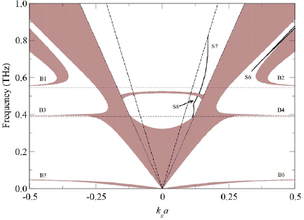
Figure 4. The same as in figure 3, but focusing on a different frequency region. Here, B1, B2, B3, B4, and B6 are labels for the bulk bands, while S6, S7, and S8 are the labels for the surface modes discussed in the text.
Download figure:
Standard image High-resolution imageIn region (b) we have a bulk region terminating at the DLL, for kx > 0 or kx < 0. In figures 3 and 4 we can also see the so-called graphene induced gap, by analogy with results in [8, 9], but in the present case the gap starts at about 0.32 THz and finishes at about 2.48 THz for kxa = 0. Naturally, this gap depends on the GPC parameters (such as layer thicknesses, dielectric constants, etc), but here we have the added feature that it depends on the applied magnetic field as well. For the case where there is zero applied magnetic field, this gap starts at the origin [9], i.e. where kxa = 0 and f = 0.
The low-frequency region (c) is shown in figure 4. Here we can see the specific behaviour for the bulk modes close to the frequency values f 1 = 0.39 THz and f 2 = 0.55 THz. The bulk bands, labeled by B1 and B2 are reciprocal and tend to f 2 when kx goes to infinity. This value represents a resonance frequency corresponding to the maximum in Im( ), or the maximum in Re(
 ). The other bulk bands, labeled by B3 and B4 are also reciprocal and they tend to f 1 at larger magnitude of kxa. Here f 1 is another resonance frequency that corresponds to the minimum in Im
 (or the minimum in Re
 ). Clearly, these bulk bands depend on the resonant frequencies f 1 and f 2, and consequently on the intensity of the applied magnetic field. These bulk modes are very different from the bulk modes in dielectric (semiconductor) PCs, as well as those reported in previous works [13, 14]. We infer that these bulk modes have this different behaviour due to the absorption, as characterized by the scattering rate
  in equation (2), in the graphene sheets. Also, we see that the applied magnetic field is a very important parameter for tuning the bulk (and surface) polariton modes in the GPC. We note the small gap region that starts at 0.32 THz and finishes at 0.51 THz, for kxa = 0, and it is limited by the lowest bulk band and the DLLs. It depends sensitively on the applied magnetic field (see figure 5). On the other hand, for low frequencies, below to 0.05 THz (or 50 GHz), we have more two bulk bands, labeled by B5 and B6 (which are reciprocal), and tend to 0.045 THz when |kxa| becomes large. The surface modes in the region (c) are also quite different. We have three surface modes, labeled by S8, S7, and S6. The mode S8 starts at f = 0.38 THz for kxa = 0.11 and finishes at f = 0.49 THz for kxa = 0.133. The surface mode S7 starts at f = 0.51 THz for kxa = 0.139 and finishes at the VLL. These modes, S8 and S7, have a behaviour that is typical for polariton surface modes when we consider the damping (or absorption) in the dielectric function [36]. Indeed, here we have taken account of an equivalent damping effect through the scattering rate
  in the optical conductivity tensor (see equations (2) and (3)). We should mention here that these surface modes are very sensitive to this parameter. For example, we will not have surface modes if
  meV.
meV.

Figure 5. The polariton frequencies below 1 THz for kxa = 0.0 plotted versus the applied magnetic field B (in T).
Download figure:
Standard image High-resolution image
The non-reciprocity aspects of the surface modes, as described above, do not change with the increasing of the magnetic field. However, these modes will be shifted (except for the surface modes S7 and S8 that will disappear). We can interpret this using figure 2, because, essentially, we have a shift in the optical conductivity (including the peaks and dips in the imaginary and real parts of  ). Therefore, we present now a study to find the behaviour of these modes for bulk bands with the applied magnetic field. This behaviour will be similar for all the spectra.
Finally, in figure 5 we show the bulk polariton modes (and the band gap) for the region below 1 THz, for kxa = 0 plotted as a function of the applied magnetic field. Here, we can see that it is possible to tune the bulk bands (and gap) by changing the applied magnetic field intensity. Note that the frequencies of these bulk bands will increase approximately linearly as a function of the applied magnetic field when kxa = 0. In general terms, we comment that the absence of an applied magnetic field in this system would make this spectrum more simple, mainly in the region around f < 0.6 THz, in figure 4. Further, we would not have surface modes for s-polarization [9] in that case, as discussed also by Albuquerque and Cottam [13, 14]. On the other hand, the bulk spectrum with applied magnetic field is rather similar to the case in the absence of an applied magnetic field for p-polarization (see [9] for more detail).
5. Conclusions
In summary, we have presented a general theory for the plasmon-polaritons in graphene PCs subjected to an external applied magnetic field. Specifically we have considered a periodic photonic crystal consisting of alternating unit cells arranged in a periodic array with embedded graphene sheets at the interfaces and a static applied magnetic field in the direction perpendicular to the layers. On comparing our results with previous work we find that the inclusion of an external magnetic field in the GPC will affect strongly the dispersion relations of the polaritons, mainly at low frequencies (below about 1 THz, for B = 1.5 T). Also, we find a novel nonreciprocity effect for the propagation of the surface modes. Further, there is the possibility of having s-polarized (TE) surface polariton modes that no have counterpart in the dispersion relations in semiconductor (or dielectric) PCs [13].
In the context of applications, we mention that surface magnetoplasmons (or magnetoplasmon polaritons) in multilayer structures are typically difficult to realize because they require very high magnetic fields. The explanation is that in order to observe the effects due to an external magnetic field for metals, for example, the frequencies would need to be of the order of 1016 Hz, which is the order of the characteristic cyclotron frequency in metals [37]. The characteristic cyclotron frequency is a function of the applied magnetic field, and, therefore, in the case of metals, it needs a magnetic field of order 103 T, which is exceptionally difficult to realize in laboratories. One solution to avoid this generally unreachable magnetic field strength is to use doped semiconductors (instead of metals) where the characteristic cyclotron frequency is in the THz regime (for a review see [38]). In this case, a more modest external magnetic field of less than 2 T will suffice. From our results, by using GPCs instead semiconductor PCs, we can see that there is the possibility for the excitation of surface and bulk magnetoplasmon polaritons in this same frequency range and the same order for the specified external magnetic field.
Acknowledgments
M S Vasconcelos thanks the Department of Physics and Astronomy at the University of Western Ontario for hospitality during his sabbatical as visiting professor. This study was financed in part by the Coordenação de Aperfeioamento de Pessoal de Nível Superior (CAPES) of Brasil (Finance Code 88881.172293/2018-01) and the Natural Sciences and Engineering Research Council (NSERC) of Canada (Grant RGPIN-2017-04429).
Appendix
Here, we provide the definitions for the matrix blocks constituting the interface matrix in equation (19). First,  and
and  , which involve the diagonal elements of the graphene conductivity tensor, are given by
We note that these matrices are similar to those in [9] for p-polarization and s-polarization, respectively. The other matrices  and
and  , which involve the off-diagonal elements of the graphene conductivity tensor, are