


1 Introduction
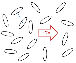
Colloidal particles diffuse down a concentration gradient at a rate that is determined by a balance between the driving force, the gradient in their chemical potential and the resistance to their motion offered by the suspending solvent (Einstein Reference Einstein1956; de Groot & Mazur Reference de Groot and Mazur1984; Russel, Saville & Schowalter Reference Russel, Saville and Schowalter1989; Felderhof Reference Felderhof2017). At infinite dilution, particle interactions of any kind are negligible, and this balance leads to the Stokes–Einstein equation (Deen Reference Deen2012). When the particle concentration is finite but small, the effect of concentration on the rate of gradient diffusion may be evaluated by using only two-particle interactions. The chemical-potential driving force is then captured by the second virial coefficient (Hill Reference Hill1960; Mulder & Frenkel Reference Mulder and Frenkel1985), and may be evaluated using expressions known from statistical thermodynamics. However, evaluation of the effect of two-particle interactions on the hydrodynamic resistance is complicated by the slow rate of decay of particle–particle interactions under the low-Reynolds-number conditions usually associated with Brownian particles.
In a series of influential papers, Batchelor (Reference Batchelor1972, Reference Batchelor1976, Reference Batchelor1983) showed that two-sphere hydrodynamic interactions can be ‘renormalized’ by using known, mean properties of a suspension, permitting the evaluation of the sedimentation velocity of suspensions of spheres to  $O(\unicode[STIX]{x1D719})$, where
  $\unicode[STIX]{x1D719}$ is particle volume fraction. Combined with the second virial coefficient of hard-sphere suspensions, the concentration-dependent sedimentation resistance yielded the prediction for the gradient or collective diffusion coefficient
  $D(\unicode[STIX]{x1D719})$:
 $$\begin{eqnarray}\displaystyle \frac{D}{D_{0}}=1+1.45\unicode[STIX]{x1D719}, & & \displaystyle\end{eqnarray}$$
 where  $D_{0}$ is the Stokes–Einstein diffusivity. An alternative derivation by Felderhof (Reference Felderhof1978) yielded a very similar result, but with the 1.45 replaced by 1.56. Here and in the text below, by gradient diffusion coefficient
  $D$ we refer to the coefficient that relates the volume flux
  $\boldsymbol{N}$ of particles to the gradient in particle volume fraction, i.e.
 $$\begin{eqnarray}\displaystyle \boldsymbol{N}=-D(\unicode[STIX]{x1D719})\unicode[STIX]{x1D735}\unicode[STIX]{x1D719}, & & \displaystyle\end{eqnarray}$$
relative to volume-fixed coordinates (i.e. the volume-average velocity is zero). More than 40 years after publication of these results, there still appears to be no published work showing how Batchelor’s method, and (1.1), are altered when the diffusing particles are not spherical. In this paper we extend Batchelor’s method to solutes that are rigid, prolate spheroids.
Significant contributions to renormalization and theories of colloidal diffusion have been made since the publications by Batchelor (Reference Batchelor1972, Reference Batchelor1976) and Felderhof (Reference Felderhof1978). Hinch (Reference Hinch1977) and O’Brien (Reference O’Brien1979) further developed and systemized averaging methods for calculating the bulk properties of suspensions. Cichocki & Felderhof (Reference Cichocki and Felderhof1988) calculated two-sphere interactions in inverse powers of the interparticle separation, and with 150 terms in the expansion obtained a result consistent with the coefficient of 1.45 in (1.1). More recently, Felderhof (Reference Felderhof2017) published an interesting overview of the generalized Einstein equation. Beenakker & Mazur (Reference Beenakker and Mazur1984) incorporated many-sphere interactions into a theory for self- and gradient diffusion that yields results at higher volume fractions than (1.1), and Cichocki et al. (Reference Cichocki, Ekiel-Jezewska, Szymczak and Wajnryb2002) derived accurate three-sphere interactions and calculated sedimentation rates to  $O(\unicode[STIX]{x1D719}^{2})$. Those theoretical results compare well with computational results obtained by implementing the method of O’Brien (Reference O’Brien1979) in Stokesian dynamics simulations (Brady et al. Reference Brady, Phillips, Lester and Bossis1988; Phillips, Brady & Bossis Reference Phillips, Brady and Bossis1988a,Reference Phillips, Brady and Bossisb). Computational results obtained by using the lattice-Boltzmann method are also in agreement with theoretical predictions at low volume fractions (Ladd Reference Ladd1994; Segre, Behrend & Pusey Reference Segre, Behrend and Pusey2016). Buck, Dungan & Phillips (Reference Buck, Dungan and Phillips1999) apply Batchelor’s method to Brinkman’s equation, and show that the resulting theory for gradient diffusion in polymer gels agrees with experimental data. A helpful compilation of existing experimental data, theoretical predictions and computational results for diffusion in hard-sphere suspensions may be found in figure 3.4 in the chapter by Zia & Brady (Reference Zia and Brady2015).
As the coefficient that relates the flux of a solute to its concentration gradient, the gradient diffusivity is of direct relevance in applications, and there are several methods for measuring it in colloidal suspensions. For example, interferometric techniques such as Rayleigh and holographic interferometry have been applied successfully to this purpose (Wakeham, Nagashima & Sengers Reference Wakeham, Nagashima and Sengers1991; Buck et al. Reference Buck, Dungan and Phillips1999; Zhang & Annunziata Reference Zhang and Annunziata2008). The Taylor dispersion method has also been used (Alizadeh, de Castro & Wakeham Reference Alizadeh, de Castro and Wakeham1980; Wakeham et al. Reference Wakeham, Nagashima and Sengers1991; Alexander, Phillips & Dungan Reference Alexander, Phillips and Dungan2019), as has a hydrodynamic instability method proposed by Taylor (Selim, Al-Naafa & Jones Reference Selim, Al-Naafa and Jones1993). For many years, dynamic light scattering (DLS) has been a very useful method for studying transport processes in colloidal suspensions, including short-time and long-time self-diffusion, and gradient or collective diffusion. The theory supporting DLS and its connection to diffusion, and the importance of time scales in defining short- and long-time self-diffusion, are described by Pusey & Tough (Reference Pusey and Tough1982) and Rallison & Hinch (Reference Rallison and Hinch1986). Pusey & Tough (Reference Pusey and Tough1982), in particular, note that to linear order in the volume fraction there is no difference between short- and long-time gradient diffusion (see the discussion below their equation (36)). Much of the data plotted by Zia & Brady (Reference Zia and Brady2015) in their figure 3.4, mentioned above, were obtained by DLS. Obtaining gradient diffusivities by DLS requires extrapolation to very small scattering vectors, which can be problematic for some systems (Segre et al. Reference Segre, Behrend and Pusey2016).
The need for rigorous theoretical results for the concentration effect on rates of diffusion of non-spherical particles is apparent when one considers that common colloidal particles and proteins are often non-spherical: bovine serum albumin (BSA), for example, a globular blood protein frequently used in laboratory experiments, has been described as a prolate spheroid with an aspect ratio that has been estimated as 1.9 (Jachimska, Wasilewska & Adamczyk Reference Jachimska, Wasilewska and Adamczyk2008) or 3.5 (Squire, Moser & O’Konski Reference Squire, Moser and O’Konski1968; Wright & Thompson Reference Wright and Thompson1975). There are also several studies that have concluded that BSA is more ‘heart shaped’, or closer to an oblate spheroid, than a prolate spheroid (Carter & Ho Reference Carter and Ho1994; Ferrer, Duchowicz & Carrasco Reference Ferrer, Duchowicz, Carrasco, de la Torre and Acuna2001; Leggio, Galantini & Pavel Reference Leggio, Galantini and Pavel2008). Rigorous results for the effect of shape on rates of diffusion can help to resolve such discrepancies. In fact, comparison of protein diffusion data with theoretical results based on hydrodynamic and excluded-volume interactions has been recommended as a means for assessing protein–protein interactions (Sorret et al. Reference Sorret, DeWinter, Schwartz and Randolph2016).
Both the chemical potential and the hydrodynamic interactions between diffusing particles are affected by a change in shape. For spherical particles, the second virial coefficient  $B_{2}$, normalized by the sphere volume, is well known to be 4,
  $B_{2}=4$. The second and third virial coefficients for prolate spheroidal particles depend on the particle aspect ratio, and have been calculated numerically by Mulder & Frenkel (Reference Mulder and Frenkel1985). Hydrodynamic interactions between two spherical particles may be described by two scalar functions of the two-sphere separation, and those functions are known to a high degree of accuracy (Stimson & Jeffery Reference Stimson and Jeffery1926; Goldman, Cox & Brenner Reference Goldman, Cox and Brenner1966; Jeffery & Onishi Reference Jeffery and Onishi1984; Kim & Mifflin Reference Kim and Mifflin1985). However, two-particle interactions between prolate spheroids are more complicated, being orientation and aspect-ratio dependent. Two-particle interactions between prolate spheroids have not been studied to nearly the same extent as two-sphere interactions, and results to the level of accuracy needed to obtain the equivalent of (1.1) for prolate spheroids are not available.
Several theoretical and numerical studies of two-spheroid interactions have been done. In the far-field limit, Kim (Reference Kim1985) used the singularity representations of Chwang & Wu (Reference Chwang and Wu1975, Reference Chwang and Wu1976), and derived solutions for two interacting spheroids to the level of the first and second reflections. His results compare well with numerical results obtained by boundary collocation for specific configurations (Gluckman, Pfeffer & Weinbaum Reference Gluckman, Pfeffer and Weinbaum1971). In addition, Claeys & Brady (Reference Claeys and Brady1993a,Reference Claeys and Bradyb) used the first reflection in Kim (Reference Kim1985), in conjunction with lubrication interactions, to develop a Stokesian-dynamics-like method for simulating the motion of spheroidal particles and suspensions.
It is worth noting that the non-Brownian sedimentation problem that provides the hydrodynamic resistance in (1.1) has no counterpart with prolate spheroidal particles. Sedimenting suspensions of non-Brownian spheroidal particles, i.e. in the high-Péclet-number limit, are unstable and become non-homogeneous during sedimentation (Koch & Shaqfeh Reference Koch and Shaqfeh1989). Partly for that reason, in their study of the hydrodynamic transport properties of suspensions of prolate spheroids, Claeys & Brady (Reference Claeys and Brady1993a,Reference Claeys and Bradyb) do not report sedimentation velocities. However, this instability does not change the fact that the mobility of a homogeneous suspension of Brownian, diffusing spheroidal particles (i.e. in the limit of small Péclet number) is needed to describe the concentration dependence of the gradient diffusion coefficient.
Here we calculate near-field two-particle interactions using the singularity method originally proposed by Dabros (Reference Dabros1985). In this method, a collection of point-force or higher-order singularities are placed within the solid particles. The strengths of these singularities are then chosen so as to impose boundary conditions on the particle surfaces (Gotz Reference Gotz2005; Phillips Reference Phillips1995; Zhou & Pozrikidis Reference Zhou and Pozrikidis1995; Phillips Reference Phillips2003), in a way that accounts for translation–rotation coupling. We have used this method previously to calculate two-sphere interactions and rates of hindered diffusion in hydrogels (Buck et al. Reference Buck, Dungan and Phillips1999; Musnicki et al. Reference Musnicki, Lloyd, Phillips and Dungan2011).
In the sections below we first summarize the renormalization method of Batchelor (Reference Batchelor1972, Reference Batchelor1976), which involves separation of two-particle far-field and near-field interactions. We then show how it can be extended to suspensions of non-spherical particles. Although for prolate spheroids the renormalized far-field interactions cannot be calculated in purely analytical form, they can be evaluated using relatively straightforward numerical methods. The near-field interactions require the more involved numerical approach using singularities placed inside the particles. We combine the far- and near-field results to compute the rate of gradient diffusion of prolate spheroidal particles to  $O(\unicode[STIX]{x1D719})$, for aspect ratios
  $\unicode[STIX]{x1D706}$ ranging from 1 (i.e. spheres) to 3.5, and compare with some experimental data from the literature in § 5.
2 Suspensions of spherical particles
We begin with a summary of the theory for the rate of gradient diffusion in suspensions of spherical particles, as that work provides the foundation for our own. Enough detail is provided so that similarities and differences between the spherical and spheroidal configurations can be identified. In the presence of a concentration gradient, particles of any shape move as if acted upon by a ‘thermodynamic force’  $\boldsymbol{F}_{\unicode[STIX]{x1D707}}$ given by (Batchelor Reference Batchelor1976)
 $$\begin{eqnarray}\displaystyle \boldsymbol{F}_{\unicode[STIX]{x1D707}}=-\frac{\unicode[STIX]{x1D735}\unicode[STIX]{x1D707}}{1-\unicode[STIX]{x1D719}}, & & \displaystyle\end{eqnarray}$$
 where  $\unicode[STIX]{x1D707}$ is the chemical potential of the diffusing particles at constant pressure and temperature. The denominator in (2.1) accounts for the enhanced motion that is contributed by the chemical potential gradient acting to push the solvent up the particle concentration gradient. Felderhof (Reference Felderhof2017) discusses and compares different expressions for the driving force for diffusion, and for colloidal suspensions arrives at a result equivalent to (2.1).
At low Reynolds number, the mean solute velocity  $\overline{\boldsymbol{U}}$ is related to this force linearly, i.e.
 $$\begin{eqnarray}\displaystyle \overline{\boldsymbol{U}}=\overline{\boldsymbol{M}}\boldsymbol{\cdot }\boldsymbol{F}_{\unicode[STIX]{x1D707}}, & & \displaystyle\end{eqnarray}$$
 where a mean particle mobility  $\overline{\boldsymbol{M}}$ has been defined. In the limit of infinite dilution,
  $\unicode[STIX]{x1D719}\rightarrow 0$, the mean mobility for spheres is found from Stokes’ solution for flow around an isolated sphere to be (Happel & Brenner Reference Happel and Brenner1986)
 $$\begin{eqnarray}\displaystyle \overline{\boldsymbol{M}}=\left(\frac{1}{6\unicode[STIX]{x03C0}\unicode[STIX]{x1D702}a}\right)\unicode[STIX]{x1D644}, & & \displaystyle\end{eqnarray}$$
 where  $\unicode[STIX]{x1D702}$ is the solvent viscosity,
  $a$ is the radius of the spherical particle and
  $\unicode[STIX]{x1D644}$ is the identity tensor.
Substituting the chemical potential of an ideal solution,
 $$\begin{eqnarray}\displaystyle \unicode[STIX]{x1D707}=\unicode[STIX]{x1D707}^{\ominus }+kT\ln \unicode[STIX]{x1D719}, & & \displaystyle\end{eqnarray}$$
 into (2.1), and using (2.2) and (2.3) at infinite dilution to obtain the flux  $\boldsymbol{N}$ of particle volume,
 $$\begin{eqnarray}\displaystyle \boldsymbol{N}=\overline{\boldsymbol{U}}\unicode[STIX]{x1D719}, & & \displaystyle\end{eqnarray}$$
shows that
 $$\begin{eqnarray}\displaystyle \boldsymbol{N}=-\left(\frac{kT}{6\unicode[STIX]{x03C0}\unicode[STIX]{x1D702}a}\right)\unicode[STIX]{x1D735}\unicode[STIX]{x1D719}. & & \displaystyle\end{eqnarray}$$
 Comparison with Fick’s law of diffusion yields the Stokes–Einstein equation for the infinite-dilution diffusivity  $D_{0}$:
 $$\begin{eqnarray}\displaystyle D_{0}=\frac{kT}{6\unicode[STIX]{x03C0}\unicode[STIX]{x1D702}a}. & & \displaystyle\end{eqnarray}$$
 In (2.4),  $\unicode[STIX]{x1D707}^{\ominus }$ is a reference chemical potential and
  $kT$ is the product of temperature and Boltzmann’s constant.
2.1 Driving force for spherical particles
At low but finite particle volume fractions,  $\unicode[STIX]{x1D719}\ll 1$, for particles of any shape the thermodynamic force
  $\boldsymbol{F}_{\unicode[STIX]{x1D707}}$ in (2.1) can be expressed using the second virial coefficient
  $B_{2}$ since
 $$\begin{eqnarray}\displaystyle \frac{\unicode[STIX]{x1D719}}{kT}\frac{\left({\displaystyle \frac{\unicode[STIX]{x2202}\unicode[STIX]{x1D707}}{\unicode[STIX]{x2202}\unicode[STIX]{x1D719}}}\right)_{P,T}}{1-\unicode[STIX]{x1D719}}=1+2B_{2}\unicode[STIX]{x1D719}. & & \displaystyle\end{eqnarray}$$
 Here  $B_{2}$ has been normalized by the particle volume. For spherical particles, from statistical thermodynamics it is known that (Hill Reference Hill1960; McQuarrie Reference McQuarrie1976)
 $$\begin{eqnarray}\displaystyle B_{2}=\frac{1}{V_{p}}\frac{1}{2}\int [1-\text{e}^{-\frac{\unicode[STIX]{x1D713}}{kT}}]\,\text{d}\boldsymbol{r}, & & \displaystyle\end{eqnarray}$$
 where  $V_{p}$ is the volume of one particle,
  $\boldsymbol{r}$ is a vector from particle 1 to particle 2 and
  $\unicode[STIX]{x1D713}$ is a position-dependent interaction energy. As mentioned above, for two spheres undergoing only steric interactions (2.9) yields a second virial coefficient equal to four,
  $B_{2}=4$.
2.2 Average mobility for spherical particles
To account for two-particle interactions in (2.2), we distinguish between the velocity  $\boldsymbol{U}_{0}$ of an isolated sphere and the velocity
  $\boldsymbol{U}(\boldsymbol{x}_{0},\boldsymbol{x}_{1})$ of a system of two identical spheres located at positions
  $\boldsymbol{x}_{0}$ and
  $\boldsymbol{x}_{1}=\boldsymbol{x}_{0}+\boldsymbol{r}$. Averaging over configurations, but neglecting three-particle interactions, yields the result (Batchelor Reference Batchelor1972)
 $$\begin{eqnarray}\displaystyle \overline{\boldsymbol{U}}=\boldsymbol{U}_{0}+\int _{\boldsymbol{r}}[\boldsymbol{U}(\boldsymbol{x}_{0},\boldsymbol{x}_{0}+\boldsymbol{r})-\boldsymbol{U}_{0}]P(\boldsymbol{x}_{0}+\boldsymbol{r}|\boldsymbol{x}_{0})\,\text{d}\boldsymbol{r}, & & \displaystyle\end{eqnarray}$$
 which is sufficient to obtain  $\overline{\boldsymbol{U}}$ to
  $O(\unicode[STIX]{x1D719})$. In (2.10), the conditional probability
  $P(\boldsymbol{x}_{0}+\boldsymbol{r}|\boldsymbol{x}_{0})$ has been used, and is defined as the probability a particle is at position
  $\boldsymbol{x}_{0}+\boldsymbol{r}$ given that the test particle is at
  $\boldsymbol{x}_{0}$. The integral is over all space, but overlapping positions are precluded by the conditional probability.
Equation (2.10) cannot be evaluated as written, because it fails to account for the unbounded nature of the suspension. This problem manifests itself mathematically through the lack of convergence of the integral on the right side. At large separations,  $r\gg a$ where
  $r=|\boldsymbol{r}|$, the conditional probability is equal to the number density
  $n$, a constant that is related to the volume fraction
  $\unicode[STIX]{x1D719}$ by
 $$\begin{eqnarray}\displaystyle \unicode[STIX]{x1D719}={\textstyle \frac{4}{3}}\unicode[STIX]{x03C0}a^{3}n. & & \displaystyle\end{eqnarray}$$
 The far-field effect of the sphere at  $\boldsymbol{x}_{1}$ on the velocity of the sphere at
  $\boldsymbol{x}_{0}$ may be evaluated by using Faxen’s law (Happel & Brenner Reference Happel and Brenner1986; Kim & Karrila Reference Kim and Karrila1991; Deen Reference Deen2012),
 $$\begin{eqnarray}\displaystyle \boldsymbol{U}(\boldsymbol{x}_{0},\boldsymbol{x}_{1})=\boldsymbol{U}_{0}+\left(1+\frac{a^{2}}{6}\unicode[STIX]{x1D6FB}^{2}\right)\boldsymbol{u}(\boldsymbol{x})|_{\boldsymbol{ x}=\boldsymbol{x}_{0}-\boldsymbol{x}_{1}}\quad (r\gg a), & & \displaystyle\end{eqnarray}$$
 where the velocity field  $\boldsymbol{u}(\boldsymbol{x})$ is the disturbance velocity at position
  $\boldsymbol{x}$ relative to an isolated sphere,
 $$\begin{eqnarray}\displaystyle \boldsymbol{u}(\boldsymbol{x})=\boldsymbol{U}_{0}\left(\frac{3a}{r}+\frac{a^{3}}{4r^{3}}\right)+\boldsymbol{U}_{0}\boldsymbol{\cdot }\frac{\boldsymbol{x}\boldsymbol{x}}{r^{3}}\left(\frac{3a}{r}-\frac{3a^{3}}{4r^{3}}\right), & & \displaystyle\end{eqnarray}$$
 and  $r=|\boldsymbol{x}|$. Substitution of (2.13) into (2.12) shows that the change in velocity of the sphere at
  $\boldsymbol{x}_{0}$ caused by the second sphere at
  $\boldsymbol{x}_{1}$ has contributions that decay as
  $1/r$ and
  $1/r^{3}$, both of which fail to converge to a finite result when integrated over unbounded space, as required by (2.10).
For reference below, it is worth noting that, for a sphere subjected to a force  $\boldsymbol{F}=6\unicode[STIX]{x03C0}\unicode[STIX]{x1D702}a\boldsymbol{U}_{0}$, an equivalent solution for
  $\boldsymbol{u}$ in (2.13) can be written as
 $$\begin{eqnarray}\displaystyle \boldsymbol{u}(\boldsymbol{x})=\left[\left(1+\frac{a^{2}}{6}\unicode[STIX]{x1D6FB}^{2}\right)\frac{\unicode[STIX]{x1D645}(\boldsymbol{x})}{8\unicode[STIX]{x03C0}\unicode[STIX]{x1D702}}\right]\boldsymbol{\cdot }\boldsymbol{F}. & & \displaystyle\end{eqnarray}$$
 Here  $\unicode[STIX]{x1D645}$ is the Oseen tensor, or point-force solution, given by
 $$\begin{eqnarray}\displaystyle \unicode[STIX]{x1D645}(\boldsymbol{x})=\left(\frac{\unicode[STIX]{x1D644}}{r}+\frac{\boldsymbol{x}\boldsymbol{x}}{r^{3}}\right). & & \displaystyle\end{eqnarray}$$
 Substitution of (2.14) into (2.12), and noting that  $\unicode[STIX]{x1D6FB}^{2}\unicode[STIX]{x1D6FB}^{2}\unicode[STIX]{x1D645}=0$, shows that the far-field interaction between a sphere at
  $\boldsymbol{r}=\boldsymbol{x}_{0}-\boldsymbol{x}_{1}$ and a second sphere at
  $\boldsymbol{x}_{1}$ is given by
 $$\begin{eqnarray}\displaystyle \boldsymbol{U}^{(1)}(\boldsymbol{x}_{0},\boldsymbol{x}_{1})-\boldsymbol{U}_{0}=\boldsymbol{F}\boldsymbol{\cdot }\left[\left(1+\frac{a^{2}}{3}\unicode[STIX]{x1D6FB}^{2}\right)\frac{\unicode[STIX]{x1D645}(\boldsymbol{x})}{8\unicode[STIX]{x03C0}\unicode[STIX]{x1D702}}\right]_{\boldsymbol{x}=\boldsymbol{x}_{0}-\boldsymbol{x}_{1}}, & & \displaystyle\end{eqnarray}$$
 where the term in square brackets is the Rotne–Prager–Yamakawa tensor (Yamakawa Reference Yamakawa1970; Rotne & Prager Reference Rotne and Prager1995). The superscript ‘ $(1)$’ in (2.16) indicates that this level of interaction is sometimes called the ‘first reflection’ (Happel & Brenner Reference Happel and Brenner1986; Kim & Karrila Reference Kim and Karrila1991).
Batchelor (Reference Batchelor1972) ‘renormalized’ the integration in (2.10) by using known, mean properties of the bulk suspension. He recognized that, although in an unbounded suspension there is no stagnant fluid far from the moving particles of interest, and no walls of a container that can be used as a reference, relative to volume-fixed coordinates the suspension-average velocity (averaged over both particle and fluid volume) must be zero. Therefore
 $$\begin{eqnarray}\displaystyle \langle \boldsymbol{u}\rangle =\int _{\boldsymbol{r}}\boldsymbol{u}(\boldsymbol{x}_{0},\boldsymbol{x}_{0}+\boldsymbol{r})P(\boldsymbol{x}_{0}+\boldsymbol{r})\,\text{d}\boldsymbol{r}=0, & & \displaystyle\end{eqnarray}$$
 where  $P(\boldsymbol{x}_{0}+\boldsymbol{r})$ is the probability of a sphere being located at position
  $\boldsymbol{x}_{0}+\boldsymbol{r}$. The integral in (2.17) is over all space; at positions inside the test particle,
  $r<a$, the velocity
  $\boldsymbol{u}$ is the sphere velocity, and at positions in the fluid it may be evaluated from (2.13). Equation (2.17) is used to renormalize the terms in Faxen’s law (2.12) that are proportional to
  $\boldsymbol{u}$.
The perturbation to the velocity of the test sphere at  $\boldsymbol{x}_{0}$ that is contributed by the Laplacian term in (2.12) must also be renormalized to achieve a convergent result. Here Batchelor (Reference Batchelor1972) argues that the mean value of the deviatoric stress
  $\unicode[STIX]{x1D749}$ must be constant in a sedimenting, statistically homogeneous suspension. Consequently, the divergence of the mean deviatoric stress must be zero, or
 $$\begin{eqnarray}\displaystyle \langle \unicode[STIX]{x1D735}\boldsymbol{\cdot }\unicode[STIX]{x1D749}\rangle =\int _{r<a}\unicode[STIX]{x1D735}\boldsymbol{\cdot }\unicode[STIX]{x1D749}(\boldsymbol{x}_{0}+\boldsymbol{r})P(\boldsymbol{x}_{0}+\boldsymbol{r})\,\text{d}\boldsymbol{r}+\int _{r>a}\unicode[STIX]{x1D735}\boldsymbol{\cdot }\unicode[STIX]{x1D749}(\boldsymbol{x}_{0}+\boldsymbol{r})P(\boldsymbol{x}_{0}+\boldsymbol{r})\,\text{d}\boldsymbol{r}=0,\quad & & \displaystyle\end{eqnarray}$$
 where the integration over all space has intentionally been separated into positions within the test sphere at  $\boldsymbol{x}_{0}$,
  $r\leqslant a$, and positions outside it,
  $r>a$. The integral over positions within the test sphere can be converted to a surface integral by using the divergence theorem.
To evaluate the integrals in (2.18) to  $O(\unicode[STIX]{x1D719})$, it is sufficient to let
  $P(\boldsymbol{x}_{0}+\boldsymbol{r})=n$ and use the deviatoric stress for an isolated spherical particle, for which on the particle surface
  $\boldsymbol{n}\boldsymbol{\cdot }\unicode[STIX]{x1D749}=-4\unicode[STIX]{x03C0}\unicode[STIX]{x1D702}a\boldsymbol{U}_{0}$, where
  $\boldsymbol{n}$ is the normal vector to the surface. Evaluation of the integral for positions inside the particle,
  $r\leqslant a$, and multiplication by
  $a^{2}/6\unicode[STIX]{x1D702}$, then permits simplification of (2.18) to
 $$\begin{eqnarray}\displaystyle \frac{a^{2}}{6\unicode[STIX]{x1D702}}\langle \unicode[STIX]{x1D735}\boldsymbol{\cdot }\unicode[STIX]{x1D749}\rangle =-\frac{\unicode[STIX]{x1D719}}{2}\boldsymbol{U}_{0}+\frac{a^{2}}{6\unicode[STIX]{x1D702}}\int _{r>a}\unicode[STIX]{x1D735}\boldsymbol{\cdot }\unicode[STIX]{x1D749}(\boldsymbol{x}_{0}+\boldsymbol{r})P(\boldsymbol{x}_{0}+\boldsymbol{r})\,\text{d}\boldsymbol{r}=0, & & \displaystyle\end{eqnarray}$$
 where (2.11) has been used. Upon using Newton’s law of viscosity, the divergence of the viscous stress becomes  $\unicode[STIX]{x1D702}\unicode[STIX]{x1D6FB}^{2}\boldsymbol{u}$. Equation (2.19) may therefore be used to renormalize terms in (2.12) that are proportional to
  $\unicode[STIX]{x1D6FB}^{2}\boldsymbol{u}$.
Summing (2.17) and (2.19) yields two terms identical in form to those obtained for  $\boldsymbol{U}-\boldsymbol{U}_{0}$ in Faxen’s law, (2.12), when substituted into (2.10). However, the suspension average velocity and stress divergence are evaluated using the probability
  $P(\boldsymbol{x}_{0})$ rather than the conditional probability
  $P(\boldsymbol{x}_{0}+\boldsymbol{r}|\boldsymbol{x}_{0})$. Summing (2.17) and (2.19), and subtracting the result (known to equal zero) from (2.10), therefore leads to
 $$\begin{eqnarray}\displaystyle \overline{\boldsymbol{U}}=\boldsymbol{U}_{0}+\overline{\boldsymbol{V}}^{\prime }+\overline{\boldsymbol{V}}^{\prime \prime }+\overline{\boldsymbol{W}}, & & \displaystyle\end{eqnarray}$$
 where  $\overline{\boldsymbol{V}}^{\prime }$ contains renormalized far-field interactions that are proportional to
  $\boldsymbol{u}$ and
  $\overline{\boldsymbol{V}}^{\prime \prime }$ contains renormalized far-field interactions that are proportional to
  $\unicode[STIX]{x1D6FB}^{2}\boldsymbol{u}$ in (2.12), respectively. The term
  $\overline{\boldsymbol{W}}$ contains all other, near-field two-sphere interactions not included in
  $\boldsymbol{V}^{\prime }$ and
  $\boldsymbol{V}^{\prime \prime }$.
The explicit expressions for the renormalized far-field terms are
 $$\begin{eqnarray}\displaystyle \overline{\boldsymbol{V}}^{\prime }=\int _{\boldsymbol{r}}\boldsymbol{u}(\boldsymbol{x}_{0},\boldsymbol{x}_{0}+\boldsymbol{r})[P(\boldsymbol{x}_{0}+\boldsymbol{r}|\boldsymbol{x}_{0})-P(\boldsymbol{x}_{0}+\boldsymbol{r})]\,\text{d}\boldsymbol{r} & & \displaystyle\end{eqnarray}$$
and
 $$\begin{eqnarray}\displaystyle \overline{\boldsymbol{V}}^{\prime \prime }=\frac{\unicode[STIX]{x1D719}\boldsymbol{U}_{0}}{2}+\int _{r>a}\frac{a^{2}}{6}\unicode[STIX]{x1D6FB}^{2}\boldsymbol{u}(\boldsymbol{x},\boldsymbol{x}_{0}+\boldsymbol{r})|_{\boldsymbol{x}=\boldsymbol{x}_{0}}[P(\boldsymbol{x}_{0}+\boldsymbol{r}|\boldsymbol{x}_{0})-P(\boldsymbol{x}_{0}+\boldsymbol{r})]\,\text{d}\boldsymbol{r}. & & \displaystyle\end{eqnarray}$$
 To the required level of accuracy both probabilities are either zero or constant, i.e.  $P(\boldsymbol{x}_{0}+\boldsymbol{r})=n$ at all positions, and the conditional probability
  $P(\boldsymbol{x}_{0}+\boldsymbol{r}|\boldsymbol{x}_{0})=n$ when
  $r\geqslant 2a$ but is zero for
  $r<2a$. As a result, the integrals in (2.21) and (2.22) are both finite, and they can be evaluated analytically using (2.13), yielding
 $$\begin{eqnarray}\displaystyle \overline{\boldsymbol{V}}^{\prime }=-{\textstyle \frac{11}{2}}\unicode[STIX]{x1D719}\boldsymbol{U}_{0} & & \displaystyle\end{eqnarray}$$
and
 $$\begin{eqnarray}\displaystyle \overline{\boldsymbol{V}}^{\prime \prime }={\textstyle \frac{1}{2}}\unicode[STIX]{x1D719}\boldsymbol{U}_{0}. & & \displaystyle\end{eqnarray}$$
Equation (2.20) then becomes
 $$\begin{eqnarray}\displaystyle \overline{\boldsymbol{U}}=\boldsymbol{U}_{0}(1-5\unicode[STIX]{x1D719})+\overline{\boldsymbol{W}}. & & \displaystyle\end{eqnarray}$$
 The near-field interactions in  $\overline{\boldsymbol{W}}$ require a solution to the complete problem of two equal spheres sedimenting in a quiescent fluid at low Reynolds number.
The function  $\boldsymbol{W}$ is formed by subtracting the far-field interaction, as obtained from Faxen’s law, (2.12), from the complete two-sphere solution
  $\boldsymbol{U}(\boldsymbol{x}+\boldsymbol{r},\boldsymbol{x})$ for the velocity of a sphere at
  $\boldsymbol{x}+\boldsymbol{r}$ in the presence of a second, equal sphere at
  $\boldsymbol{x}$, i.e.
 $$\begin{eqnarray}\displaystyle \boldsymbol{W}(\boldsymbol{x}_{0},\boldsymbol{x}_{0}+\boldsymbol{r})=\boldsymbol{U}(\boldsymbol{x}_{0},\boldsymbol{x}_{0}+\boldsymbol{r})-\boldsymbol{U}_{0}-\left[1+\frac{a^{2}}{6}\unicode[STIX]{x1D6FB}^{2}\right]\boldsymbol{u}(\boldsymbol{x},\boldsymbol{x}_{0}+\boldsymbol{r})|_{\boldsymbol{x}=\boldsymbol{x}_{0}}. & & \displaystyle\end{eqnarray}$$
 The term with square brackets in (2.26) could equivalently be replaced by the right side of (2.16). The average of  $\boldsymbol{W}$ is then defined by
 $$\begin{eqnarray}\displaystyle \overline{\boldsymbol{W}}=n\int _{r\geqslant 2a}\boldsymbol{W}(\boldsymbol{x}_{0},\boldsymbol{x}_{0}+\boldsymbol{r})\,\text{d}\boldsymbol{r}. & & \displaystyle\end{eqnarray}$$
 The functions defining the detailed two-sphere interaction  $\boldsymbol{U}(\boldsymbol{x}_{0},\boldsymbol{x}_{0}+\boldsymbol{r})$ were obtained to a high level of accuracy by Stimson & Jeffery (Reference Stimson and Jeffery1926) and Goldman et al. (Reference Goldman, Cox and Brenner1966), and Batchelor (Reference Batchelor1972) used them to evaluate
  $\overline{\boldsymbol{W}}$, obtaining
 $$\begin{eqnarray}\displaystyle \overline{\boldsymbol{W}}=-1.55\unicode[STIX]{x1D719}. & & \displaystyle\end{eqnarray}$$
With (2.25), the mean sedimentation velocity is then
 $$\begin{eqnarray}\displaystyle \overline{\boldsymbol{U}}=\boldsymbol{U}_{0}(1-6.55\unicode[STIX]{x1D719}). & & \displaystyle\end{eqnarray}$$
 For reference below, we note that the slowest decaying interaction in  $\boldsymbol{W}(\boldsymbol{x}_{0},\boldsymbol{x}_{0}+\boldsymbol{r})$ is contributed by the stresslet on the sphere at
  $\boldsymbol{x}_{0}+\boldsymbol{r}$ that is caused by the test sphere at
  $\boldsymbol{x}_{0}$. This ‘second-reflection’ contribution changes the velocity of the sphere at
  $\boldsymbol{x}_{0}$ by
  $-\boldsymbol{U}_{0}(15a^{4})/(4r^{4})$, a result that may be used to evaluate contributions to
  $\overline{\boldsymbol{W}}$ from sphere–sphere separations so large that numerical calculation becomes impractical. In his calculation, Batchelor (Reference Batchelor1972) truncates the numerical integration in (2.27) at
  $r=8a$, and evaluates the contribution from
  $r>8a$ by using the asymptotic, second-reflection result. A similar approach is used below for spheroidal particles.
Returning to the flux defined in (2.5), and calculating the mean solute velocity  $\overline{\boldsymbol{U}}$ using the force
  $\boldsymbol{F}_{\unicode[STIX]{x1D707}}$ in (2.1) and 2.8, we obtain
 $$\begin{eqnarray}\displaystyle D(\unicode[STIX]{x1D719})=D_{0}(1+2B_{2}\unicode[STIX]{x1D719})(1-6.55\unicode[STIX]{x1D719}). & & \displaystyle\end{eqnarray}$$
 Using  $B_{2}=4$ for spherical solutes undergoing only steric interactions, to
  $O(\unicode[STIX]{x1D719})$ one finds that
 $$\begin{eqnarray}\displaystyle D(\unicode[STIX]{x1D719})=D_{0}(1+1.45\unicode[STIX]{x1D719}), & & \displaystyle\end{eqnarray}$$
 which was first derived by Batchelor (Reference Batchelor1976). The diffusivity  $D(\unicode[STIX]{x1D719})$ in (2.31) is the coefficient given in (1.2). To linear order in volume fraction, it describes the diffusive flux of particle volume in a Brownian suspension of hard spheres, relative to a volume-fixed reference frame.
3 Suspensions of prolate spheroidal particles
The thermodynamic driving force for diffusion given in (2.1), and the relation between the mean solute velocity and the flux in (2.5), are independent of particle shape. In order to extend the analysis in § 2 to prolate spheroidal particles, it is therefore necessary to obtain results for the chemical potential and average mobility comparable to (2.8), (2.9) and (2.29).
3.1 Particle shape
By ‘prolate spheroid’ we refer to an object that is elongated along an axis of symmetry, such that points on the surface  $\boldsymbol{x}_{s}$ are given by
 $$\begin{eqnarray}\displaystyle \frac{(x_{s,1}-x_{c,1})^{2}}{b^{2}}+\frac{(x_{s,2}-x_{c,2})^{2}}{b^{2}}+\frac{(x_{s,3}-x_{c,3})^{2}}{a^{2}}=1 & & \displaystyle\end{eqnarray}$$
 for a particle centred at  $\boldsymbol{x}_{c}$. Equation (3.1) describes a prolate spheroid with a major axis of half-length
  $a$, i.e.
  $a>b$, aligned with the
  $z$, or
  $x_{3}$, axis. The minor axes have half-length
  $b$. For the special case
  $a=b$, (3.1) reduces to the equation describing a sphere with radius
  $a$, whereas for a spheroid the aspect ratio
  $\unicode[STIX]{x1D706}=a/b>1$. A more general description of a prolate spheroidal particle, centred at
  $\boldsymbol{x}_{c}$ but with arbitrary orientation, is given by
 $$\begin{eqnarray}\displaystyle (\boldsymbol{x}-\boldsymbol{x}_{c})\boldsymbol{\cdot }\left[\frac{1}{b^{2}}(\boldsymbol{e}_{1}\boldsymbol{e}_{1}+\boldsymbol{e}_{2}\boldsymbol{e}_{2})+\frac{1}{a^{2}}\boldsymbol{d}\boldsymbol{d}\right]\boldsymbol{\cdot }(\boldsymbol{x}-\boldsymbol{x}_{c})=1, & & \displaystyle\end{eqnarray}$$
 where the unit vector  $\boldsymbol{d}$ is in the direction of the major axis, the axis of symmetry, and the unit vectors
  $\boldsymbol{e}_{1}$ and
  $\boldsymbol{e}_{2}$ are orthogonal to
  $\boldsymbol{d}$ and to each other.
3.2 Driving force for prolate spheroids
Evaluation of the second virial coefficient for prolate spheroids is more complicated than for spheres, because as non-isotropic particles they have a clearly defined orientation  $\boldsymbol{d}$. For prolate spheroidal particles undergoing only steric interactions, Mulder & Frenkel (Reference Mulder and Frenkel1985) have derived an expression for the second virial coefficient by means of statistical thermodynamics, and they show that
 $$\begin{eqnarray}\displaystyle B_{2}=-\frac{1}{2(4\unicode[STIX]{x03C0})^{2}}\int \text{d}\boldsymbol{r}\int \int \text{d}\unicode[STIX]{x1D6FA}_{0}\,\text{d}\unicode[STIX]{x1D6FA}_{1}f(\boldsymbol{r},\boldsymbol{d}_{0},\boldsymbol{d}_{1}), & & \displaystyle\end{eqnarray}$$
 where  $\boldsymbol{r}$ is the centre-to-centre vector between the particles, and
  $\boldsymbol{d}_{0}$ and
  $\boldsymbol{d}_{1}$ (or angles contained in
  $\unicode[STIX]{x1D6FA}_{0}$ and
  $\unicode[STIX]{x1D6FA}_{1}$) define their orientations. The function
  $f(\boldsymbol{r},\boldsymbol{d}_{0},\boldsymbol{d}_{1})$ is the Mayer function, and for hard particles equals
  $-1$ if they overlap and zero otherwise. The integration over the particle orientation angles
  $\unicode[STIX]{x1D6FA}_{k}$ requires consideration of all orientations
  $\boldsymbol{d}_{k}$. However, because only two particles are involved and the surrounding medium is isotropic, it is sufficient to fix one particle and obtain all two-particle configurations by changing the position and orientation of the other. It has been assumed in (3.3) that the particles are equally likely to have any non-overlapping orientation, so that their orientational distribution functions are normalized by
  $4\unicode[STIX]{x03C0}$.
We define a conditional probability  $P_{p}(\boldsymbol{x}_{1},\unicode[STIX]{x1D6FA}_{1}|\boldsymbol{x}_{0},\unicode[STIX]{x1D6FA}_{0})$ as the probability that a particle is at position
  $\boldsymbol{x}_{1}$ with orientation
  $\unicode[STIX]{x1D6FA}_{1}$, given that a test particle is at position
  $\boldsymbol{x}_{0}$ with orientation
  $\unicode[STIX]{x1D6FA}_{0}$. Under dilute conditions, when the particle separation is greater than
  $2a$,
$2a$,  $r>2a$, this conditional probability is
  $n/4\unicode[STIX]{x03C0}$. Averaged over all possible orientations
  $\unicode[STIX]{x1D6FA}_{0}$ and
  $\unicode[STIX]{x1D6FA}_{1}$, we denote the average by
  $\overline{P}_{p}(\boldsymbol{x}_{0}+\boldsymbol{r}|\boldsymbol{x}_{0})$, which is a function of
  $r=|\boldsymbol{r}|$ only, where
  $\boldsymbol{r}=\boldsymbol{x}_{1}-\boldsymbol{x}_{0}$. In terms of the Mayer function,
 $$\begin{eqnarray}\displaystyle \overline{P}_{p}(\boldsymbol{x}_{0}+\boldsymbol{r}|\boldsymbol{x}_{0})=\frac{1}{(4\unicode[STIX]{x03C0})^{2}}\int \int \text{d}\unicode[STIX]{x1D6FA}_{0}\,\text{d}\unicode[STIX]{x1D6FA}_{1}f(\boldsymbol{r},\boldsymbol{d}_{0},\boldsymbol{d}_{1}). & & \displaystyle\end{eqnarray}$$
Comparison with (3.3) shows that
 $$\begin{eqnarray}\displaystyle B_{2}=-\frac{1}{2}\int \text{d}\boldsymbol{r}\overline{P}_{p}(\boldsymbol{x}_{0}+\boldsymbol{r}|\boldsymbol{x}_{0}). & & \displaystyle\end{eqnarray}$$
 In the development of Mulder & Frenkel (Reference Mulder and Frenkel1985) it is convenient to reverse the order of integration relative to that shown in (3.3). Doing the integration over relative particle-to-particle separations  $\boldsymbol{r}$ first is useful, because Isihara (Reference Isihara1951) derived an explicit expression for the excluded volume of two prolate spheroids with fixed orientations. Although using
  $\overline{P}_{p}(\boldsymbol{x}_{0}+\boldsymbol{r}|\boldsymbol{x}_{0})$ precludes use of the analytic result of Isihara (Reference Isihara1951), and therefore yields slightly less accurate results, the orientation-averaged conditional probability in (3.4) is needed in the hydrodynamic renormalization procedure below.
A plot of  $\overline{P}_{p}(\boldsymbol{x}_{0}+\boldsymbol{r}|\boldsymbol{x}_{0})$ for values of
  $\unicode[STIX]{x1D706}$ of 1.25, 2.0 and 3.0 is given in figure 1. For a dilute suspension of spherical particles, for which
  $b=a$, the function plotted,
  $1-\overline{P}_{p}/n$, would fall vertically from 1.0 to zero at
  $r=2b$. For hard spheroidal particles, it is still impossible for two particle centres to be closer than
  $2b$, but in the region
  $2b\leqslant r\leqslant 2a$, some orientations are permitted and others are excluded because they correspond to particle overlap. All of the curves become zero for
  $r>2\unicode[STIX]{x1D706}b$, but for spheroids the decay is gradual rather than abrupt as it is for spherical particles.
Evaluation of the integral in (3.4) requires an efficient method for determining when two spheroidal particles overlap. For two identical spheroids, Perram & Wertheim (Reference Perram and Wertheim1985) propose such an algorithm that is computationally efficient and accurate. They define a scalar ‘contact function’ based on the positions and orientations of the particles. The maximum value of the contact function is shown to be unique, and when it is less than one they show that the particles must overlap. We calculated the maximum value numerically using Brent’s method (Press et al. Reference Press, Flannery, Teukolsky and Vetterling1989), and evaluated the integrals in (3.4) numerically by using the trapezoid rule. Our results for  $B_{2}$, normalized by the particle volume, agree with those in table 1 of the paper by Mulder & Frenkel (Reference Mulder and Frenkel1985), and are shown in our table 1.

Figure 1. Plot of  $1-\overline{P}_{p}/n$ versus
  $r/b$ for
  $\unicode[STIX]{x1D706}=1.25$, 2.0 and 3.0. Results decay to zero for
  $r/b>2\unicode[STIX]{x1D706}$, where
  $\unicode[STIX]{x1D706}=a/b$.
Table 1. Second virial coefficients for spheroidal particles.

3.3 Far-field interactions between spheroidal particles
Extending the dilute-limit, two-particle ensemble average for sedimentation velocity to account for orientation, the equation for prolate spheroidal particles corresponding to (2.10) is
 $$\begin{eqnarray}\displaystyle \overline{\boldsymbol{U}}_{p} & = & \displaystyle \overline{\boldsymbol{U}}_{p,0}+\int _{\boldsymbol{r}}\int _{\unicode[STIX]{x1D6FA}_{0}}\int _{\unicode[STIX]{x1D6FA}_{1}}[\boldsymbol{U}_{p}(\boldsymbol{x}_{0},\unicode[STIX]{x1D6FA}_{0},\boldsymbol{x}_{0}+\boldsymbol{r},\unicode[STIX]{x1D6FA}_{1})-\boldsymbol{U}_{p,0}]\nonumber\\ \displaystyle & & \displaystyle \times \,P_{p}(\boldsymbol{x}_{0}+\boldsymbol{r},\unicode[STIX]{x1D6FA}_{1}|\boldsymbol{x}_{0},\unicode[STIX]{x1D6FA}_{0})\,\text{d}\unicode[STIX]{x1D6FA}_{0}\,\text{d}\unicode[STIX]{x1D6FA}_{1}\,\text{d}\boldsymbol{r}.\end{eqnarray}$$
 Here, the orientations are accounted for explicitly through their two orientation angles, represented by  $\unicode[STIX]{x1D6FA}_{0}$ and
  $\unicode[STIX]{x1D6FA}_{1}$, and a subscript ‘
 $p$’ indicates a quantity for a spheroidal, rather than a spherical, particle. The overbar on
  $\boldsymbol{U}_{p,0}$ in (3.6) implies an orientation average over an isolated particle. The relation between volume fraction and number density for the spheroidal particles comparable to (2.11) is
 $$\begin{eqnarray}\displaystyle \unicode[STIX]{x1D719}={\textstyle \frac{4}{3}}\unicode[STIX]{x03C0}b^{2}an. & & \displaystyle\end{eqnarray}$$
 Because we consider two-particle interactions only, we require that the volume fraction be low,  $\unicode[STIX]{x1D719}\ll 1$. However, for elongated particles with large aspect ratio
  $\unicode[STIX]{x1D706}\gg 1$, the more stringent requirement that
  $\unicode[STIX]{x1D719}\unicode[STIX]{x1D706}^{2}\ll 1$ must also be satisfied.
As the velocity disturbance for any particle, regardless of shape, is given by the point-force disturbance  $\unicode[STIX]{x1D645}\boldsymbol{\cdot }\boldsymbol{F}$ (cf. (2.14)) at positions far from it, two-particle interactions for spheroids must have a slowly decaying
  $1/r$ interaction just as is present with spherical particles. Renormalization is therefore required. However, the precise nature of how to achieve it depends on the detailed nature of the two-particle interactions. In particular, the
  $1/r^{3}$ interaction term for spherical particles is shape dependent, and a comparable term for non-spherical particles must therefore likewise be shape dependent.
3.3.1 First-reflection interactions between spheroidal particles
The low-Reynolds-number disturbance velocity caused by isolated prolate spheroidal particles, and interactions between two such particles, have been of interest for some time, and results for large separations and specific configurations were obtained by Wakaya (Reference Wakaya1965) and Gluckman et al. (Reference Gluckman, Pfeffer and Weinbaum1971), among others. For our purposes the paper by Kim (Reference Kim1985), which relies heavily on the contributions of Chwang & Wu (Reference Chwang and Wu1975, Reference Chwang and Wu1976), is particularly useful. With it we can evaluate the form of all non-convergent far-field interactions between two spheroidal particles, permitting selection of a suitable method of renormalization. For spherical particles these non-convergent interactions are given in (2.16), and Kim (Reference Kim1985) provides the corresponding ‘first-reflection’ result for spheroids. Stresslet-level interactions, or the ‘second reflection’ for distant particles, are also very useful in permitting the longest-range convergent interactions to be accounted for analytically.
The relation between the force  $\boldsymbol{F}$ and velocity
  $\boldsymbol{U}_{p,0}$ of an isolated spheroidal particle is given by
 $$\begin{eqnarray}\displaystyle \boldsymbol{U}_{p,0}=\frac{\boldsymbol{F}}{6\unicode[STIX]{x03C0}\unicode[STIX]{x1D702}a}\boldsymbol{\cdot }\left[\frac{1}{X^{A}}\boldsymbol{d}\boldsymbol{d}+\frac{1}{Y^{A}}(\unicode[STIX]{x1D644}-\boldsymbol{d}\boldsymbol{d})\right], & & \displaystyle\end{eqnarray}$$
 where the parameters  $X^{A}$ and
  $Y^{A}$ are (Kim & Karrila Reference Kim and Karrila1991)
 $$\begin{eqnarray}\displaystyle X^{A}=\frac{8}{3}\unicode[STIX]{x1D716}^{3}\left[-2\unicode[STIX]{x1D716}+(1+\unicode[STIX]{x1D716}^{2})\ln \left(\frac{1+\unicode[STIX]{x1D716}}{1-\unicode[STIX]{x1D716}}\right)\right]^{-1} & & \displaystyle\end{eqnarray}$$
and
 $$\begin{eqnarray}\displaystyle Y^{A}=\frac{16}{3}\unicode[STIX]{x1D716}^{3}\left[2\unicode[STIX]{x1D716}+(3\unicode[STIX]{x1D716}^{2}-1)\ln \left(\frac{1+\unicode[STIX]{x1D716}}{1-\unicode[STIX]{x1D716}}\right)\right]^{-1}. & & \displaystyle\end{eqnarray}$$
 Here,  $\unicode[STIX]{x1D716}$ is the spheroid eccentricity, related to the aspect ratio
  $\unicode[STIX]{x1D706}=a/b$ by
 $$\begin{eqnarray}\displaystyle \unicode[STIX]{x1D716}=[1-\unicode[STIX]{x1D706}^{-2}]^{1/2}. & & \displaystyle\end{eqnarray}$$
For diffusion over time scales long enough that the isolated particle samples all orientations, an isotropic mobility relates the particle force and velocity. Averaging (3.8) over all possible orientations yields
 $$\begin{eqnarray}\displaystyle \overline{\boldsymbol{U}}_{p,0}=\frac{\boldsymbol{F}}{6\unicode[STIX]{x03C0}\unicode[STIX]{x1D702}a}\left(\frac{1}{3}\frac{1}{X^{A}}+\frac{2}{3}\frac{1}{Y^{A}}\right) & & \displaystyle\end{eqnarray}$$
 from which the average mobility in (2.2) in the limit  $\unicode[STIX]{x1D719}\rightarrow 0$ follows directly.
The fluid velocity disturbance  $\boldsymbol{u}_{p}$ at position
  $\boldsymbol{x}$ caused by an isolated spheroid with centre at
  $\boldsymbol{x}_{1}$ that is subject to a force
  $\boldsymbol{F}$ is given by (Kim Reference Kim1985)
 $$\begin{eqnarray}\displaystyle \boldsymbol{u}_{p}(\boldsymbol{x},\boldsymbol{x}_{1})=\boldsymbol{F}\boldsymbol{\cdot }\int _{-k}^{k}\frac{\text{d}\unicode[STIX]{x1D709}}{2\unicode[STIX]{x1D716}a}\left[1+(\unicode[STIX]{x1D716}^{2}a^{2}-\unicode[STIX]{x1D709}^{2})\frac{1-\unicode[STIX]{x1D716}^{2}}{4\unicode[STIX]{x1D716}^{2}}\unicode[STIX]{x1D6FB}^{2}\right]\frac{\unicode[STIX]{x1D645}(\boldsymbol{x}-\unicode[STIX]{x1D743}_{1})}{8\unicode[STIX]{x03C0}\unicode[STIX]{x1D702}}\,\text{d}\unicode[STIX]{x1D709}, & & \displaystyle\end{eqnarray}$$
 where  $k=\unicode[STIX]{x1D716}a$. As shown in figure 2, in (3.13)
  $\unicode[STIX]{x1D743}_{1}$ is a position along the axis of symmetry of the particle, and the integration extends from one focus to the other. This result corresponds to
  $\boldsymbol{u}$ in (2.13) and (2.14) for an isolated sphere, and it is particularly interesting to compare with (2.14). Equation (2.14) shows that the velocity disturbance from a sphere subject to a force
  $\boldsymbol{F}$ is a point-force velocity disturbance
  $\unicode[STIX]{x1D645}\boldsymbol{\cdot }\boldsymbol{F}$ added to a quadrupole contribution proportional to
  $\unicode[STIX]{x1D6FB}^{2}\unicode[STIX]{x1D645}$. Equation (3.1) has the same structure, but the disturbance velocity is contributed by a line distribution of point forces and quadrupoles.
As discussed by Kim (Reference Kim1985), the first-reflection description of the effect of one spheroidal particle’s motion on a second particle, corresponding to (2.12) with (2.13) or (2.16) for spheres, is given by
 $$\begin{eqnarray}\displaystyle \boldsymbol{U}^{(1)} & = & \displaystyle \frac{\boldsymbol{F}}{8\unicode[STIX]{x03C0}\unicode[STIX]{x1D702}}\boldsymbol{\cdot }\int _{-k}^{k}\frac{\text{d}\unicode[STIX]{x1D709}_{0}}{2k}\int _{-k}^{k}\frac{\text{d}\unicode[STIX]{x1D709}_{1}}{2k}\left[1+(k^{2}-\unicode[STIX]{x1D709}_{0}^{2})\frac{(1-e^{2})}{4e^{2}}\unicode[STIX]{x1D6FB}^{2}\right.\nonumber\\ \displaystyle & & \displaystyle \left.+(k^{2}-\unicode[STIX]{x1D709}_{1}^{2})\frac{(1-e^{2})}{4e^{2}}\unicode[STIX]{x1D6FB}^{2}\right]\unicode[STIX]{x1D645}(\boldsymbol{x})|_{\boldsymbol{x}=\boldsymbol{y}_{0}-\boldsymbol{y}_{1}}.\end{eqnarray}$$
 Equation (3.14) describes the far-field effect of a spheroid at position  $\boldsymbol{x}_{1}$ on a second, identical, test spheroid at
  $\boldsymbol{x}_{0}$. Positions along the axes of symmetry of the spheroids are given by the vectors
  $\boldsymbol{y}_{1}$ and
  $\boldsymbol{y}_{0}$, respectively. The vectors from a particle centre to a point along the axis of symmetry of the same particle are given by
 $$\begin{eqnarray}\displaystyle \unicode[STIX]{x1D743}_{i}=\boldsymbol{y}_{i}-\boldsymbol{x}_{i}, & & \displaystyle\end{eqnarray}$$
 where  $i=0$ for the test particle and
  $i=1$ for the other particle. The magnitudes of distance along the axes are then
  $\unicode[STIX]{x1D709}_{0}=|\unicode[STIX]{x1D743}_{0}-\boldsymbol{x}_{0}|$ for the particle at
  $\boldsymbol{x}_{0}$ and
  $\unicode[STIX]{x1D709}_{1}=|\unicode[STIX]{x1D743}_{1}-\boldsymbol{x}_{1}|$ for the particle at
  $\boldsymbol{x}_{1}$. The two integrations proceed from point to point along the particle axes, from one focus at
  $k=-a\unicode[STIX]{x1D716}$ to the other at
  $k=+a\unicode[STIX]{x1D716}$. The force
  $\boldsymbol{F}$ can be related to the velocity of an isolated particle upon which it acts by using (3.8).

Figure 2. Schematic diagram of the two spheroidal particles with centres at  $\boldsymbol{x}_{0}$ (the test particle) and
  $\boldsymbol{x}_{1}$. A line along the axis of symmetry extends between the foci, from
  $\unicode[STIX]{x1D709}_{i}=-k$ to
  $\unicode[STIX]{x1D709}_{i}=+k$, where
  $i=0$ or
  $i=1$,
  $k=a\unicode[STIX]{x1D716}$ and
  $\unicode[STIX]{x1D709}_{i}=|\unicode[STIX]{x1D743}_{i}|$.
When the distance between two particles is large compared to their long dimension  $a$,
$a$,  $r=|\boldsymbol{x}_{0}-\boldsymbol{x}_{1}|\gg a$, the contributions from one point along the particle axis asymptotically approaches those from other points. Thus a far-field simplification to (3.13) can be obtained by using Taylor expansions of the Oseen tensor
  $\unicode[STIX]{x1D645}$ about
  $\boldsymbol{x}_{0}-\boldsymbol{x}_{1}$, with the corrections being caused by the separation between points on the axes and the particle centres,
 $$\begin{eqnarray}\displaystyle (\boldsymbol{y}_{0}-\boldsymbol{y}_{1})-(\boldsymbol{x}_{0}-\boldsymbol{x}_{1})=\unicode[STIX]{x1D743}_{0}-\unicode[STIX]{x1D743}_{1}. & & \displaystyle\end{eqnarray}$$
Then the expansion is
 $$\begin{eqnarray}\displaystyle \unicode[STIX]{x1D645}(\boldsymbol{y}_{0}-\boldsymbol{y}_{1}) & {\approx} & \displaystyle \unicode[STIX]{x1D645}(\boldsymbol{x}_{0}-\boldsymbol{x}_{1})+(\unicode[STIX]{x1D743}_{0}-\unicode[STIX]{x1D743}_{1})\boldsymbol{\cdot }\unicode[STIX]{x1D735}\unicode[STIX]{x1D645}|_{\boldsymbol{x}_{0}-\boldsymbol{x}_{1}}\nonumber\\ \displaystyle & & \displaystyle +\frac{1}{2}(\unicode[STIX]{x1D743}_{0}-\unicode[STIX]{x1D743}_{1})(\unicode[STIX]{x1D743}_{0}-\unicode[STIX]{x1D743}_{1}):\unicode[STIX]{x1D735}\unicode[STIX]{x1D735}\unicode[STIX]{x1D645}|_{\boldsymbol{x}_{0}-\boldsymbol{x}_{1}}+\cdots\end{eqnarray}$$
 Substitution of (3.17) into the first-reflection expression (3.14) yields a result in which the particle orientations are only present in the vectors  $\unicode[STIX]{x1D743}_{0}-\unicode[STIX]{x1D743}_{1}$.
Since far-field approximations are applicable when the particles are well separated,  $r>2a$, the interacting particles are free to sample all possible orientations. The result obtained by substituting (3.17) into (3.14) can therefore be simplified by averaging over all particle orientations, using that
 $$\begin{eqnarray}\displaystyle \overline{\unicode[STIX]{x1D743}_{0}-\unicode[STIX]{x1D743}_{1}}=\overline{\unicode[STIX]{x1D743}_{0}}-\overline{\unicode[STIX]{x1D743}_{1}}=0 & & \displaystyle\end{eqnarray}$$
and
 $$\begin{eqnarray}\displaystyle \overline{(\unicode[STIX]{x1D743}_{0}-\unicode[STIX]{x1D743}_{1})(\unicode[STIX]{x1D743}_{0}-\unicode[STIX]{x1D743}_{1})}={\textstyle \frac{1}{3}}(\unicode[STIX]{x1D709}_{0}^{2}+\unicode[STIX]{x1D709}_{1}^{2})\unicode[STIX]{x1D644}. & & \displaystyle\end{eqnarray}$$
In addition, the Oseen tensor and its gradients are evaluated at the particle centres, and may be removed from the integrals. Substitution of (3.17) into (3.14), simplification of the result using (3.18) and (3.19), and doing the integrations, yields the result
 $$\begin{eqnarray}\displaystyle \overline{\boldsymbol{U}}^{(1)}=\boldsymbol{F}_{1}\boldsymbol{\cdot }\left[1+\frac{b^{2}}{3}\left(1+\frac{\unicode[STIX]{x1D706}^{2}\unicode[STIX]{x1D716}^{2}}{3}\right)\unicode[STIX]{x1D6FB}^{2}\right]\unicode[STIX]{x1D645}(\boldsymbol{x})|_{\boldsymbol{ x}=\boldsymbol{x}_{0}-\boldsymbol{x}_{1}}. & & \displaystyle\end{eqnarray}$$
 Comparison of (3.20) with (2.16) shows that, in the far-field limit, the orientation-averaged interaction between prolate spheroids is asymptotically equivalent to that between spheres with radii  $b_{R}$, where
 $$\begin{eqnarray}\displaystyle b_{R}^{2}=b^{2}[1+(1/3)(\unicode[STIX]{x1D706}\unicode[STIX]{x1D716})^{2}] & & \displaystyle\end{eqnarray}$$
or, equivalently, using (3.11),
 $$\begin{eqnarray}\displaystyle b_{R}=b[1+(1/3)(\unicode[STIX]{x1D706}^{2}-1)]^{1/2}. & & \displaystyle\end{eqnarray}$$
 If  $\unicode[STIX]{x1D706}=1$ and
  $\unicode[STIX]{x1D716}=0$, the particles are interacting spheres, and (3.20) is equivalent to (2.16) for two equal spheres with radii equal to
  $a$ or
  $b$.
$b$.
Although the diffusing species are prolate spheroids, all that is required for renormalization is entities that undergo the same far-field interactions, and therefore we choose to renormalize the spheroid interactions using spheres with radius  $b_{R}$. The renormalization suspension comprised of spheres has the same number density as the actual suspension of prolate spheroidal particles, and each sphere in the renormalization suspension is subjected to the same force as one of the prolate spheroidal particles. In isolation their sedimentation velocity is therefore
 $$\begin{eqnarray}\displaystyle \boldsymbol{U}_{R}=\frac{\boldsymbol{F}}{6\unicode[STIX]{x03C0}\unicode[STIX]{x1D707}b_{R}}. & & \displaystyle\end{eqnarray}$$
 The velocity disturbance from one of the renormalization spheres is  $\boldsymbol{u}_{R}$, and in isolation can be evaluated with either (2.13) or (2.14), with the radius
  $a$ replaced by
  $b_{R}$.
3.3.2 Second-reflection interactions between spheroidal particles
Equation (3.14) describes how the velocity disturbance from one spheroidal particle, say Particle 1 at  $\boldsymbol{x}_{1}$, calculated as if it were the only particle, affects the velocity of the test particle at
  $\boldsymbol{x}_{0}$, or the ‘first reflection’. The next level of interaction, the second reflection, accounts for the fact that the presence of the test particle at
  $\boldsymbol{x}_{0}$ alters the stress distribution on the surface of Particle 1. That change in the surface stress gives rise to a stresslet velocity disturbance that reflects back and alters the velocity of the test particle. The slowest decaying stresslet disturbance decays as
  $1/r^{4}$, rather than
  $1/r$ or
  $1/r^{3}$ as is the case with the first-reflection terms.
Although interactions to the level of the first reflection, as given by (3.14), are all that is required to renormalize the sedimentation problem, it is very helpful to have the slowest decaying portion of the second-reflection contribution in analytical form. Upon integration over three-dimensional space, the stresslet interaction that decays as  $1/r^{4}$ is multiplied by
  $r^{2}$, and therefore has a significant impact on the sedimentation velocity, even for regions far from the test particle where numerical calculation of the interaction is computationally costly. In the calculation by Batchelor (Reference Batchelor1972), the asymptotic result for this second reflection is used to account for two-sphere interactions for which
  $r>8a$, and yields a contribution of
  $-0.47\unicode[STIX]{x1D719}\boldsymbol{U}_{0}$ to the overall total (from
  $\boldsymbol{W}$) of
  $-1.55\unicode[STIX]{x1D719}\boldsymbol{U}_{0}$.
We therefore found it convenient, even necessary, to obtain the corresponding asymptotic result for prolate spheroidal particles. Since it is far-field interactions that are required, only the orientation-averaged interaction is needed, and all orientations are accessible because the separation is greater than  $2a$. To obtain our results, we use somewhat lengthy expressions derived by Kim (Reference Kim1985), that simplify considerably when orientation averaged and only the slowest decaying interaction is required.
The stresslet on Particle 1, located at  $\boldsymbol{x}_{1}$ with orientation
  $\boldsymbol{d}_{1}$ is, in indicial notation,
 $$\begin{eqnarray}\displaystyle \frac{S_{1,ij}^{(1)}}{8\unicode[STIX]{x03C0}\unicode[STIX]{x1D702}} & = & \displaystyle \left[-\frac{1}{2}\unicode[STIX]{x1D6FC}_{5}\left(d_{1,i}d_{1,j}-\frac{1}{3}\unicode[STIX]{x1D6FF}_{ij}\right)\left(d_{1,k}d_{1,\ell }-\frac{1}{3}\unicode[STIX]{x1D6FF}_{k\ell }\right)\right.\nonumber\\ \displaystyle & & \displaystyle -\frac{1}{4}\unicode[STIX]{x1D6FC}^{\ast }(d_{1,i}\unicode[STIX]{x1D6FF}_{jk}d_{1,\ell }+d_{1,i}\unicode[STIX]{x1D6FF}_{j\ell }d_{1,k}+\unicode[STIX]{x1D6FF}_{i\ell }d_{1,j}d_{1,k}\unicode[STIX]{x1D6FF}_{ik}d_{1,j}d_{1,\ell }-4d_{1,i}d_{1,j}d_{1,k}d_{1,\ell })\nonumber\\ \displaystyle & & \displaystyle -\frac{1}{2}\unicode[STIX]{x1D6FC}_{4} (\unicode[STIX]{x1D6FF}_{ik}\unicode[STIX]{x1D6FF}_{j\ell }+\unicode[STIX]{x1D6FF}_{i\ell }\unicode[STIX]{x1D6FF}_{jk}+\unicode[STIX]{x1D6FF}_{ij}d_{1,k}d_{1,\ell }+d_{1,i}d_{1,j}d_{1,k}d_{1,\ell }\nonumber\\ \displaystyle & & \displaystyle \left.-d_{1,i}\unicode[STIX]{x1D6FF}_{jk}d_{1,\ell }-d_{1,i}\unicode[STIX]{x1D6FF}_{j\ell }d_{1,k}-\unicode[STIX]{x1D6FF}_{i\ell }d_{1,j}d_{1,k}-\unicode[STIX]{x1D6FF}_{ik}d_{1,j}d_{1,\ell } )\right]\nonumber\\ \displaystyle & & \displaystyle \times \int _{-k}^{k}(k^{2}-\unicode[STIX]{x1D709}_{1}^{2})E_{0,k\ell }(\unicode[STIX]{x1D709}_{1})\,\text{d}\unicode[STIX]{x1D709}_{1}-\frac{\unicode[STIX]{x1D6FE}^{\ast }}{4}(d_{1,i}\unicode[STIX]{x1D716}_{jk\ell }d_{1,\ell }+d_{1,j}\unicode[STIX]{x1D716}_{ik\ell }d_{1,\ell })\nonumber\\ \displaystyle & & \displaystyle \times \int _{-k}^{k}(k^{2}-\unicode[STIX]{x1D709}_{1}^{2})[\unicode[STIX]{x1D735}\times \boldsymbol{u}_{p,0}(\unicode[STIX]{x1D743}_{1})_{k}-2\unicode[STIX]{x1D714}_{1,k}^{(1)}]\,\text{d}\unicode[STIX]{x1D709}_{1}.\end{eqnarray}$$
 In (3.24),  $\boldsymbol{S}_{1}^{(1)}$ is the stresslet on the particle at
  $\boldsymbol{x}_{1}$ caused by the velocity disturbance from the test particle at
  $\boldsymbol{x}_{0}$. The stresslet forms in response to the rate of strain
  $\boldsymbol{E}_{p}$ contributed by the test particle,
 $$\begin{eqnarray}\displaystyle \boldsymbol{E}_{p}={\textstyle \frac{1}{2}}(\unicode[STIX]{x1D735}\boldsymbol{u}_{p,0}+\unicode[STIX]{x1D735}\boldsymbol{u}_{p,0}^{t}), & & \displaystyle\end{eqnarray}$$
 integrated at points a distance  $\unicode[STIX]{x1D709}_{1}$ from
  $\boldsymbol{x}_{1}$ along the axis of symmetry of Particle 1. In the derivation of Kim (Reference Kim1985), there is an additional contribution from
  $\unicode[STIX]{x1D6FB}^{2}\boldsymbol{E}_{p}$ that has been omitted here because it decays faster than
  $\boldsymbol{E}_{p}$.
The parameter  $\unicode[STIX]{x1D6FE}^{\ast }$ in (3.24) is (Chwang & Wu Reference Chwang and Wu1975)
 $$\begin{eqnarray}\displaystyle \unicode[STIX]{x1D6FE}^{\ast }=\unicode[STIX]{x1D6FE}_{3}-\unicode[STIX]{x1D6FE}_{3}^{\prime }, & & \displaystyle\end{eqnarray}$$
where
 $$\begin{eqnarray}\displaystyle \unicode[STIX]{x1D6FE}_{3}=(1-\unicode[STIX]{x1D716}^{2})\left[-2\unicode[STIX]{x1D716}+(1+\unicode[STIX]{x1D716}^{2})\ln \left(\frac{1+\unicode[STIX]{x1D716}}{1-\unicode[STIX]{x1D716}}\right)\right]^{-1} & & \displaystyle\end{eqnarray}$$
and
 $$\begin{eqnarray}\displaystyle \unicode[STIX]{x1D6FE}_{3}^{\prime }=\unicode[STIX]{x1D6FE}_{3}(1-\unicode[STIX]{x1D716}^{2})^{-1}. & & \displaystyle\end{eqnarray}$$
 The  $\unicode[STIX]{x1D6FC}$ parameters are (Chwang & Wu Reference Chwang and Wu1975)
 $$\begin{eqnarray}\displaystyle & \displaystyle \unicode[STIX]{x1D6FC}_{3}=\unicode[STIX]{x1D6FE}_{3}\frac{2\unicode[STIX]{x1D716}^{2}\left[-2\unicode[STIX]{x1D716}+\ln \left({\displaystyle \frac{1+\unicode[STIX]{x1D716}}{1-\unicode[STIX]{x1D716}}}\right)\right]}{\left[2\unicode[STIX]{x1D716}(2\unicode[STIX]{x1D716}^{2}-3)+3(1-\unicode[STIX]{x1D716}^{2})\ln \left({\displaystyle \frac{1+\unicode[STIX]{x1D716}}{1-\unicode[STIX]{x1D716}}}\right)\right]}, & \displaystyle\end{eqnarray}$$
 $$\begin{eqnarray}\displaystyle & \displaystyle \unicode[STIX]{x1D6FC}_{3}^{\prime }=\unicode[STIX]{x1D6FE}_{3}^{\prime }\frac{\unicode[STIX]{x1D716}^{2}\left[-2\unicode[STIX]{x1D716}+(1-\unicode[STIX]{x1D716}^{2})\ln \left({\displaystyle \frac{1+\unicode[STIX]{x1D716}}{1-\unicode[STIX]{x1D716}}}\right)\right]}{\left[2\unicode[STIX]{x1D716}(2\unicode[STIX]{x1D716}^{2}-3)+3(1-\unicode[STIX]{x1D716}^{2})\ln \left({\displaystyle \frac{1+\unicode[STIX]{x1D716}}{1-\unicode[STIX]{x1D716}}}\right)\right]}, & \displaystyle\end{eqnarray}$$
 $$\begin{eqnarray}\displaystyle & \displaystyle \unicode[STIX]{x1D6FC}^{\ast }=\unicode[STIX]{x1D6FC}_{3}-\unicode[STIX]{x1D6FC}_{3}^{\prime }, & \displaystyle\end{eqnarray}$$
 $$\begin{eqnarray}\displaystyle & \displaystyle \unicode[STIX]{x1D6FC}_{4}=2\unicode[STIX]{x1D716}^{2}(1-\unicode[STIX]{x1D716}^{2})\left[2\unicode[STIX]{x1D716}(3-5\unicode[STIX]{x1D716}^{2})-3(1-\unicode[STIX]{x1D716}^{2})^{2}\ln \left(\frac{1+\unicode[STIX]{x1D716}}{1-\unicode[STIX]{x1D716}}\right)\right]^{-1}, & \displaystyle\end{eqnarray}$$
and
 $$\begin{eqnarray}\displaystyle \unicode[STIX]{x1D6FC}_{5}=\unicode[STIX]{x1D716}^{2}\left[6\unicode[STIX]{x1D716}-(3-\unicode[STIX]{x1D716}^{2})\ln \left(\frac{1+\unicode[STIX]{x1D716}}{1-\unicode[STIX]{x1D716}}\right)\right]^{-1}. & & \displaystyle\end{eqnarray}$$
 For reference below, we note that for spherical particles, the eccentricity vanishes,  $\unicode[STIX]{x1D716}\rightarrow 0$, and in that limit
 $$\begin{eqnarray}\displaystyle & \displaystyle \unicode[STIX]{x1D6FE}^{\ast }=-{\textstyle \frac{3}{8\unicode[STIX]{x1D716}}}, & \displaystyle\end{eqnarray}$$
 $$\begin{eqnarray}\displaystyle & \displaystyle \unicode[STIX]{x1D6FC}_{4}=-{\textstyle \frac{5}{8\unicode[STIX]{x1D716}^{3}}}, & \displaystyle\end{eqnarray}$$
 $$\begin{eqnarray}\displaystyle & \displaystyle \unicode[STIX]{x1D6FC}_{5}=-{\textstyle \frac{15}{8\unicode[STIX]{x1D716}^{3}}}, & \displaystyle\end{eqnarray}$$
and
 $$\begin{eqnarray}\displaystyle \unicode[STIX]{x1D6FC}^{\ast }=-{\textstyle \frac{5}{4\unicode[STIX]{x1D716}^{3}}}. & & \displaystyle\end{eqnarray}$$
These results are useful for making comparison with known results for spheres.
To average (3.24) over the possible orientations of Particle 1, we use that
 $$\begin{eqnarray}\displaystyle \overline{\boldsymbol{d}\boldsymbol{d}}={\textstyle \frac{1}{3}}\unicode[STIX]{x1D644} & & \displaystyle\end{eqnarray}$$
and, in indicial notation,
 $$\begin{eqnarray}\displaystyle \overline{d_{i}d_{j}d_{k}d_{\ell }}={\textstyle \frac{1}{15}}(\unicode[STIX]{x1D6FF}_{ij}\unicode[STIX]{x1D6FF}_{k\ell }+\unicode[STIX]{x1D6FF}_{ik}\unicode[STIX]{x1D6FF}_{j\ell }+\unicode[STIX]{x1D6FF}_{i\ell }\unicode[STIX]{x1D6FF}_{kj}), & & \displaystyle\end{eqnarray}$$
 where overbars again indicate averaging over orientation. In addition, the rotational velocity  $\unicode[STIX]{x1D74E}_{1}$ in the last integral of (3.24) is given by (see Kim (Reference Kim1985), equation [3.11], noting changes to notation)
 $$\begin{eqnarray}\displaystyle \unicode[STIX]{x1D74E}_{1} & = & \displaystyle \frac{3}{8(ae)^{3}}\int _{-k}^{k}(k^{2}-\unicode[STIX]{x1D709}_{1}^{2})\unicode[STIX]{x1D735}\times \boldsymbol{u}_{p,0}(\unicode[STIX]{x1D709}_{1})\,\text{d}\unicode[STIX]{x1D709}_{1}\nonumber\\ \displaystyle & & \displaystyle +\frac{3}{4k^{3}}\frac{e^{2}}{2-e^{2}}\int _{-k}^{k}(k^{2}-\unicode[STIX]{x1D709}_{1}^{2})[\boldsymbol{d}_{1}\times (\boldsymbol{E}_{p}(\unicode[STIX]{x1D709}_{1})\boldsymbol{\cdot }\boldsymbol{d}_{1})]\,\text{d}\unicode[STIX]{x1D709}_{1}.\end{eqnarray}$$
 To obtain only the slowest decaying contribution to  $\boldsymbol{S}_{1}^{(1)}$, the vorticity terms
  $\unicode[STIX]{x1D735}\times \boldsymbol{u}_{p,0}$ in (3.24) and (3.40) may be evaluated at the particle centre
  $\unicode[STIX]{x1D709}_{1}=0$, and the result is independent of
  $\boldsymbol{d}_{1}$. Because the prefactor averages to zero,
 $$\begin{eqnarray}\displaystyle \overline{d_{1,i}\unicode[STIX]{x1D716}_{jk\ell }d_{1,\ell }+d_{1,j}\unicode[STIX]{x1D716}_{ik\ell }d_{1,\ell }}=0, & & \displaystyle\end{eqnarray}$$
those terms make no contribution to the orientation-averaged result.
To obtain the slowest decaying interaction from the second reflection, it is sufficient to neglect the variation of  $E_{p,k\ell }$ and
  $\unicode[STIX]{x1D714}_{1,i}^{1}$ along the axis of Particle 1, permitting the integrals over
  $\unicode[STIX]{x1D709}_{1}$ to be evaluated analytically. After some algebra, one arrives at the result
 $$\begin{eqnarray}\displaystyle \frac{\overline{S}_{1,ij}^{(1),\infty }}{8\unicode[STIX]{x03C0}\unicode[STIX]{x1D702}}=-\left(\frac{4}{3}\unicode[STIX]{x1D716}^{3}a^{3}\right)\overline{\unicode[STIX]{x1D6FC}}E_{p,ij}^{\infty }(\boldsymbol{x}_{1}), & & \displaystyle\end{eqnarray}$$
where
 $$\begin{eqnarray}\displaystyle \overline{\unicode[STIX]{x1D6FC}}=\frac{\unicode[STIX]{x1D6FC}_{5}}{15}+\frac{\unicode[STIX]{x1D6FC}^{\ast }}{5}+\frac{2}{5}\unicode[STIX]{x1D6FC}_{4}-\left(\frac{\unicode[STIX]{x1D716}^{2}}{2-\unicode[STIX]{x1D716}^{2}}\right)\frac{\unicode[STIX]{x1D6FE}^{\ast }}{5}. & & \displaystyle\end{eqnarray}$$
 Equation (3.42) provides  $O(a^{2}r^{-2})$, orientation-averaged contributions to the stresslet on Particle 1 caused by the test particle. The superscript
  $\infty$ indicates that it is valid in the far-field limit, because contributions from
  $\unicode[STIX]{x1D6FB}^{2}\boldsymbol{E}_{p}$ have been neglected.
Substitution of the parameters in the limit the spheroids become spheres,  $\unicode[STIX]{x1D716}\rightarrow 0$, given in (3.34)–(3.37), yields the result
 $$\begin{eqnarray}\displaystyle \overline{\unicode[STIX]{x1D6FC}}=-{\textstyle \frac{5}{8\unicode[STIX]{x1D716}^{3}}}\quad (\unicode[STIX]{x1D716}\rightarrow 0) & & \displaystyle\end{eqnarray}$$
and hence
 $$\begin{eqnarray}\displaystyle \overline{S}_{1,ij}^{(1),\infty }={\textstyle \frac{20}{3}}\unicode[STIX]{x03C0}\unicode[STIX]{x1D702}a^{3}E_{p,ij}^{\infty }(\boldsymbol{x}_{1})\quad (\unicode[STIX]{x1D716}\rightarrow 0), & & \displaystyle\end{eqnarray}$$
 where  $\boldsymbol{E}_{p}$ is the rate of strain caused by the test particle, evaluated at the centre of Particle 1. Equation (3.45) is the well-known result that yields, for example, the Einstein correction to the viscosity of a dilute suspension of hard spheres.
To proceed we evaluate  $\boldsymbol{E}_{p}^{\infty }$ using (3.25) and the
  $O(ar^{-1})$ contribution to
  $\boldsymbol{u}_{p,0}$ in (3.13), which is
 $$\begin{eqnarray}\displaystyle \boldsymbol{u}_{p,0}^{\infty }=\frac{1}{8\unicode[STIX]{x03C0}\unicode[STIX]{x1D702}}\unicode[STIX]{x1D645}\boldsymbol{\cdot }\boldsymbol{F}. & & \displaystyle\end{eqnarray}$$
The result is
 $$\begin{eqnarray}\displaystyle \boldsymbol{E}_{p}^{\infty }(\boldsymbol{r})=\frac{1}{8\unicode[STIX]{x03C0}\unicode[STIX]{x1D702}}\left[\frac{1}{r^{3}}\unicode[STIX]{x1D644}\boldsymbol{r}-\frac{3}{r^{5}}\boldsymbol{r}\boldsymbol{r}\boldsymbol{r}\right]\boldsymbol{\cdot }\boldsymbol{F}, & & \displaystyle\end{eqnarray}$$
 where  $\boldsymbol{r}=\boldsymbol{x}_{1}-\boldsymbol{x}_{0}$. This contribution to the rate of strain at
  $\boldsymbol{x}_{1}$ causes a stresslet on the particle there, that in turn yields a fluid velocity disturbance that alters the velocity
  $\boldsymbol{U}_{p}$ of the test particle by an amount (cf. equation [3.8] in Kim (Reference Kim1985))
 $$\begin{eqnarray}\displaystyle \boldsymbol{U}_{p}^{(2),\infty }=\left[\frac{1}{8\unicode[STIX]{x03C0}\unicode[STIX]{x1D702}}\int _{-k}^{k}\frac{\text{d}\unicode[STIX]{x1D709}_{0}}{2k}\int _{-k}^{k}\frac{3}{4}\frac{\text{d}\unicode[STIX]{x1D709}_{1}}{k^{3}}(k^{2}-\unicode[STIX]{x1D709}_{1}^{2})\right]\frac{3}{r^{5}}\boldsymbol{r}\boldsymbol{r}\boldsymbol{r}:\overline{\boldsymbol{S}}_{1}^{(1),\infty }. & & \displaystyle\end{eqnarray}$$
 Substitution of the rate of strain  $\boldsymbol{E}_{p}^{\infty }$ from (3.47) into (3.42), and the resulting stresslet
  $\overline{\boldsymbol{S}}_{1}^{(1),\infty }$ into (3.48), and evaluating the integrals over
  $\unicode[STIX]{x1D709}_{0}$ and
  $\unicode[STIX]{x1D709}_{1}$, shows that
 $$\begin{eqnarray}\displaystyle \overline{\boldsymbol{U}}_{p}^{(2),\infty }=\frac{k^{3}\overline{\unicode[STIX]{x1D6FC}}}{\unicode[STIX]{x03C0}\unicode[STIX]{x1D702}}\frac{\boldsymbol{r}\boldsymbol{r}}{r^{6}}\boldsymbol{\cdot }\boldsymbol{F}. & & \displaystyle\end{eqnarray}$$
 Equation (3.49) yields the slowest decaying effect of the orientation-averaged stresslet induced on the particle at  $\boldsymbol{x}_{1}$ on the motion of the test particle at
  $\boldsymbol{x}_{0}$. We note that, to this level of approximation, the result is independent of the orientation of the test particle.
To obtain the asymptotic form of the second reflection that accounts for the combined effect of all distant particles, one can multiply by the number density  $n$ of particles, and integrate over positions farther than a cutoff, say
  $r>r\ast$. Then the net far-field effect is
 $$\begin{eqnarray}\displaystyle \boldsymbol{F}\boldsymbol{\cdot }\int _{\unicode[STIX]{x1D6FA}}\int _{r\ast }^{\infty }\frac{nk^{3}\overline{\unicode[STIX]{x1D6FC}}}{\unicode[STIX]{x03C0}\unicode[STIX]{x1D702}}\frac{\boldsymbol{r}\boldsymbol{r}}{r^{6}}r^{2}\,\text{d}r\,\text{d}\unicode[STIX]{x1D6FA}=\boldsymbol{F}\int _{r\ast }^{\infty }\frac{4nk^{3}\overline{\unicode[STIX]{x1D6FC}}}{3\unicode[STIX]{x1D702}}r^{-2}\,\text{d}r, & & \displaystyle\end{eqnarray}$$
 where the expression on the right is obtained by doing the integration over the solid angle  $\unicode[STIX]{x1D6FA}$. In terms of the velocity of an isolated sphere with radius
  $a$,
$a$,  $\boldsymbol{U}_{0}=\boldsymbol{F}/6\unicode[STIX]{x03C0}\unicode[STIX]{x1D702}a$, and using (3.7) and that
  $k=a\unicode[STIX]{x1D716}$, the far-field effect in (3.50) takes the form
 $$\begin{eqnarray}\displaystyle \boldsymbol{U}_{0}\unicode[STIX]{x1D719}\int _{r\ast }^{\infty }6(\unicode[STIX]{x1D706}^{2}\unicode[STIX]{x1D716}^{3}\overline{\unicode[STIX]{x1D6FC}})\frac{a^{2}}{r^{2}}d\left(\frac{r}{a}\right). & & \displaystyle\end{eqnarray}$$
 In the limit the particles become spheres,  $\unicode[STIX]{x1D716}\rightarrow 0$, (3.44) can be used to find
  $\overline{\unicode[STIX]{x1D6FC}}$. Under those conditions, the integrals in (3.50) become
 $$\begin{eqnarray}\displaystyle -\boldsymbol{U}_{0}\unicode[STIX]{x1D719}\int _{r\ast }^{\infty }\frac{15a^{2}}{4r^{2}}d\left(\frac{r}{a}\right), & & \displaystyle\end{eqnarray}$$
 which is the result for spheres mentioned below (2.29), and is discussed below (5.7) in Batchelor’s analysis for spherical particles (Batchelor Reference Batchelor1972). Values of  $\unicode[STIX]{x1D706}^{2}\unicode[STIX]{x1D716}^{3}\overline{\unicode[STIX]{x1D6FC}}$ at several eccentricities of interest here are provided in table 2.
Table 2. Values of  $\unicode[STIX]{x1D706}^{2}\unicode[STIX]{x1D716}^{3}\overline{\unicode[STIX]{x1D6FC}}$.

3.4 Renormalizing spheroidal particle interactions
With (3.20), it is clear that the non-convergent interactions in (3.6) for spheroidal particles are interactions that decay as  $1/r$ and
  $1/r^{3}$, just as is the case for spherical particles. In fact, when rotationally averaged, the interactions between spheroidal particles are asymptotically equivalent to those between spheres if the sphere radius is chosen appropriately. We can therefore renormalize the integral in (3.6) by applying (2.17) and (2.18), in which the average velocity and divergence of the deviatoric stress are equated to zero, to a suspension of sedimenting spheres with radii
  $b_{R}=b[1+(1/3)(\unicode[STIX]{x1D706}\unicode[STIX]{x1D716})^{2}]^{1/2}$.
To effect the renormalization, we first subtract the orientation-averaged, far-field two-particle interaction  $\boldsymbol{U}_{p}^{(1)}$ from the complete two-particle interaction
  $\boldsymbol{U}_{p}$ to define
  $\boldsymbol{W}_{p}$ as
 $$\begin{eqnarray}\displaystyle \boldsymbol{W}_{p}(\boldsymbol{x}_{0},\unicode[STIX]{x1D6FA}_{0},\boldsymbol{x}_{0}+\boldsymbol{r},\unicode[STIX]{x1D6FA}_{1})=\boldsymbol{U}_{p}(\boldsymbol{x}_{0},\unicode[STIX]{x1D6FA}_{0},\boldsymbol{x}_{0}+\boldsymbol{r},\unicode[STIX]{x1D6FA}_{1})-\left[1+\frac{b_{R}^{2}}{6}\unicode[STIX]{x1D6FB}^{2}\right]\boldsymbol{u}_{R}. & & \displaystyle\end{eqnarray}$$
 Equation (3.53) is analogous to the definition of  $\boldsymbol{W}$ in (2.26). The contribution
  $\boldsymbol{W}_{p}$ contains only near-field interactions, because the slowly converging parts of the interaction have been subtracted out. In a form analogous to (2.20), we write
 $$\begin{eqnarray}\displaystyle \overline{\boldsymbol{U}}_{p}=\overline{\boldsymbol{U}}_{p,0}+\overline{\boldsymbol{V}}_{p}+\overline{\boldsymbol{W}}_{p} & & \displaystyle\end{eqnarray}$$
 in which the average of  $\boldsymbol{W}_{p}$ is
 $$\begin{eqnarray}\displaystyle \overline{\boldsymbol{W}}_{p}=\overline{\boldsymbol{U}}_{p,0}+\int _{\boldsymbol{r}}\int _{\unicode[STIX]{x1D6FC}}\int _{\unicode[STIX]{x1D6FA}_{0}}\boldsymbol{W}_{p}(\boldsymbol{x}_{0},\unicode[STIX]{x1D6FA}_{0},\boldsymbol{x}_{0}+\boldsymbol{r},\unicode[STIX]{x1D6FA}_{1})P_{p}(\boldsymbol{x}_{0}+\boldsymbol{r},\unicode[STIX]{x1D6FA}_{1}|\boldsymbol{x}_{0},\unicode[STIX]{x1D6FA}_{0})\,\text{d}\unicode[STIX]{x1D6FA}_{0}\,\text{d}\unicode[STIX]{x1D6FA}_{1}\,\text{d}\boldsymbol{r},\qquad & & \displaystyle\end{eqnarray}$$
 the position and orientation of the test particle are denoted by  $\boldsymbol{x}_{0}$ and
  $\unicode[STIX]{x1D6FA}_{0}$, respectively, and the position and orientation of the second particle by
  $\boldsymbol{x}_{0}+\boldsymbol{r}$ and
  $\unicode[STIX]{x1D6FA}_{1}$, respectively. The single-particle, orientation-averaged sedimentation velocity
  $\overline{\boldsymbol{U}}_{p,0}$ is given by (3.12).
The convergence difficulties lie in  $\overline{\boldsymbol{V}}_{p}$, which we separate into two parts as in the sphere renormalization problem,
 $$\begin{eqnarray}\displaystyle \overline{\boldsymbol{V}}_{p}=\boldsymbol{V}_{p}^{\prime }+\boldsymbol{V}_{p}^{\prime \prime }. & & \displaystyle\end{eqnarray}$$
 Here the interaction between two renormalization spheres that is proportional to  $\boldsymbol{u}_{R}$ in (2.12) is contained in the
  $\boldsymbol{V}_{p}^{\prime }$ term, and the interaction that is proportional to
  $\unicode[STIX]{x1D6FB}^{2}\boldsymbol{u}_{R}$, is in the
  $\boldsymbol{V}_{p}^{\prime \prime }$ term. The detailed expression for
  $\boldsymbol{V}_{p}^{\prime }$ is
 $$\begin{eqnarray}\displaystyle \boldsymbol{V}_{p}^{\prime }=\int _{\boldsymbol{r}}\int _{\unicode[STIX]{x1D6FC}}\int _{\unicode[STIX]{x1D6FA}_{0}}\boldsymbol{u}_{R}(\boldsymbol{x}_{0},\boldsymbol{x}_{0}+\boldsymbol{r})P_{p}(\boldsymbol{x}_{0}+\boldsymbol{r},\unicode[STIX]{x1D6FA}_{0}+\unicode[STIX]{x1D6FC}|\boldsymbol{x}_{0},\unicode[STIX]{x1D6FA}_{0})\,\text{d}\unicode[STIX]{x1D6FA}_{0}\,\text{d}\unicode[STIX]{x1D6FC}\,\text{d}\boldsymbol{r}, & & \displaystyle\end{eqnarray}$$
 and for  $\boldsymbol{V}_{p}^{\prime \prime }$ we have
 $$\begin{eqnarray}\displaystyle \boldsymbol{V}_{p}^{\prime \prime }=\int _{\boldsymbol{r}}\int _{\unicode[STIX]{x1D6FC}}\int _{\unicode[STIX]{x1D6FA}_{0}}\frac{b_{R}^{2}}{6}\unicode[STIX]{x1D6FB}^{2}\boldsymbol{u}_{R}(\boldsymbol{x},\boldsymbol{x}_{0}+\boldsymbol{r})|_{\boldsymbol{x}=\boldsymbol{x}_{0}}P_{p}(\boldsymbol{x}_{0}+\boldsymbol{r},\unicode[STIX]{x1D6FA}_{0}+\unicode[STIX]{x1D6FC}|\boldsymbol{x}_{0},\unicode[STIX]{x1D6FA}_{0})\,\text{d}\unicode[STIX]{x1D6FA}_{0}\,\text{d}\unicode[STIX]{x1D6FC}\,\text{d}\boldsymbol{r}. & & \displaystyle\end{eqnarray}$$
Equations (3.57) and (3.58) contain non-convergent integrals and cannot be evaluated without renormalization.
Since the velocity field  $\boldsymbol{u}_{R}$ corresponds to the perturbation from a renormalization sphere and is independent of orientation, the integrals over orientation in (3.57) can be applied only to the probability function
  $P_{p}$ to yield
  $\overline{P}_{p}(\boldsymbol{x}_{0}+\boldsymbol{r}|\boldsymbol{x}_{0})$ as in (3.4). Making that simplification, and subtracting off the renormalization quantity from (2.17), in this case given by
 $$\begin{eqnarray}\displaystyle \langle \boldsymbol{u}_{R}\rangle =\int _{\boldsymbol{r}}\boldsymbol{u}_{R}(\boldsymbol{x}_{0},\boldsymbol{x}_{0}+\boldsymbol{r})P_{R}(\boldsymbol{x}_{0}+\boldsymbol{r})\,\text{d}\boldsymbol{r}=0, & & \displaystyle\end{eqnarray}$$
 with the probability distribution for the renormalization spheres  $P_{R}=n$, one obtains
 $$\begin{eqnarray}\displaystyle \boldsymbol{V}_{p}^{\prime }=\int _{\boldsymbol{r}}\boldsymbol{u}_{R}(\boldsymbol{x}_{0},\boldsymbol{x}_{1})[\overline{P}_{p}(\boldsymbol{x}_{0}+\boldsymbol{r}|\boldsymbol{x}_{0})-n]\,\text{d}\boldsymbol{r}. & & \displaystyle\end{eqnarray}$$
 Equation (3.60) is the renormalized result for  $\boldsymbol{V}_{p}^{\prime }$ corresponding to (2.21) for spheres.
Comparing (3.60) and (2.21), one sees that in both cases an integral over all space that is not convergent has been reduced to a convergent integral over a finite region. However, in (2.21) the difference  $P(\boldsymbol{x}_{0}+\boldsymbol{r}|\boldsymbol{x}_{0})-n$ is either equal to
  $-n$ for
  $r\leqslant 2a$ or zero for
  $r>2a$. By contrast, in (3.60) there are three regions, as is evident in figure 1. The orientation-averaged conditional probability
  $\overline{P}_{p}$ depends only on the distance
  $r$ from the test particle, and
 $$\begin{eqnarray}\displaystyle \overline{P}_{p}-n=\left\{\begin{array}{@{}ll@{}}-n & r<b,\\ g(r) & b\leqslant r\leqslant 2a,\\ 0 & r>2a.\end{array}\right. & & \displaystyle\end{eqnarray}$$
 The function  $g(r)$ must be found numerically, and can be integrated to obtain the second virial coefficient, as discussed below (3.5).
Incorporating (3.61) into (3.60) yields a more detailed result for  $\boldsymbol{V}_{p}^{\prime }$:
 $$\begin{eqnarray}\displaystyle \boldsymbol{V}_{p}^{\prime } & = & \displaystyle -\frac{4}{3}\unicode[STIX]{x03C0}b^{3}n\boldsymbol{U}_{R}+\boldsymbol{U}_{R}\int _{b<r<b_{R}}[\overline{P}_{p}(\boldsymbol{x}_{0}+\boldsymbol{r}|\boldsymbol{x}_{0})-n]\,\text{d}\boldsymbol{r}\nonumber\\ \displaystyle & & \displaystyle +\int _{b_{R}<r<2a}\boldsymbol{u}_{R}(\boldsymbol{x}_{0},\boldsymbol{x}_{1})[\overline{P}_{p}(\boldsymbol{x}_{0}+\boldsymbol{r}|\boldsymbol{x}_{0})-n]\,\text{d}\boldsymbol{r}.\end{eqnarray}$$
 Equation (3.62) reflects the fact that, inside the renormalization spheres where  $r<b_{R}$, the velocity is
  $\boldsymbol{U}_{R}$. The orientation-averaged conditional probability
  $\overline{P}_{p}$ is zero in the region
  $r<b$, but is equal to a function of the radial distance
  $r$ from the test particle (cf. figure 1) in the region
  $b<r<b_{R}$. Finally, in the region outside the radius of the renormalization sphere,
  $b_{R}<r<2a$, the velocity
  $\boldsymbol{u}_{R}$ is given by (2.13) (or 2.14) with
  $a$ replaced by
  $b_{R}$, and the orientation-averaged probability is finite. Outside the region where the particles could overlap, i.e. where
  $r>2a$, the integrand is zero because the number densities of the renormalization spheres and prolate spheroidal particles are the same.
Recognizing that the angular integration of  $\boldsymbol{u}_{R}$ is given by
 $$\begin{eqnarray}\displaystyle \int _{\unicode[STIX]{x1D6FA}}\boldsymbol{u}_{R}\,\text{d}\unicode[STIX]{x1D6FA}=4\unicode[STIX]{x03C0}\boldsymbol{U}_{R}\left(\frac{b_{R}}{r}\right), & & \displaystyle\end{eqnarray}$$
 the contribution  $\boldsymbol{V}_{p}^{\prime }$ in (3.62) can be simplified to
 $$\begin{eqnarray}\displaystyle \boldsymbol{V}_{p}^{\prime }=-\unicode[STIX]{x1D719}\boldsymbol{U}_{R}\left[\frac{1}{\unicode[STIX]{x1D706}}+3\unicode[STIX]{x1D706}^{2}I_{1}+3\unicode[STIX]{x1D706}^{2}\hat{b}_{R}I_{2}\right], & & \displaystyle\end{eqnarray}$$
where
 $$\begin{eqnarray}\displaystyle I_{1}=\int _{1/\unicode[STIX]{x1D706}<\hat{r}<\hat{b}_{R}}[1-g(\hat{r})]\hat{r}^{2}\,\text{d}\hat{r} & & \displaystyle\end{eqnarray}$$
and
 $$\begin{eqnarray}\displaystyle I_{2}=\int _{\hat{b}_{R}<\hat{r}<2}[1-g(\hat{r})]\hat{r}\,\text{d}\hat{r}. & & \displaystyle\end{eqnarray}$$
 Here, the radial function  $g(\hat{r})$ is
  $\overline{P}_{p}/n$, the dimensionless radial position
  $\hat{r}=r/a$, and the dimensionless radius of the renormalization spheres is
  $\hat{b}_{R}=b_{R}/a$. Numerical results for
  $I_{1}$ and
  $I_{2}$ are given in table 3.


We now turn to the evaluation of  $\boldsymbol{V}_{p}^{\prime \prime }$. The mean divergence of the deviatoric stress must be zero in the renormalization suspension of sedimenting spheres, just as it is in an actual suspension of sedimenting spheres. We therefore have
 $$\begin{eqnarray}\displaystyle \frac{b_{R}^{2}}{6\unicode[STIX]{x1D702}}\langle \unicode[STIX]{x1D735}\boldsymbol{\cdot }\unicode[STIX]{x1D749}_{R}\rangle =-\frac{\unicode[STIX]{x1D719}_{R}}{2}\boldsymbol{U}_{R}+\frac{b_{R}^{2}}{6\unicode[STIX]{x1D702}}\int _{r>b_{R}}\unicode[STIX]{x1D735}\boldsymbol{\cdot }\unicode[STIX]{x1D749}_{R}(\boldsymbol{x}_{0}+\boldsymbol{r})P_{R}(\boldsymbol{x}_{0}+\boldsymbol{r})\,\text{d}\boldsymbol{r}=0, & & \displaystyle\end{eqnarray}$$
 where again  $P_{R}(\boldsymbol{x}_{0}+\boldsymbol{r})=n$ and
  $\unicode[STIX]{x1D719}_{R}=4\unicode[STIX]{x03C0}nb_{R}^{3}/3$. We note that the evaluation of the first term on the right side of (3.67) follows from the surface stress
  $\boldsymbol{n}\boldsymbol{\cdot }\unicode[STIX]{x1D749}_{R}$ in exactly the same way as in Batchelor’s original work (Batchelor Reference Batchelor1972), except that in the renormalization suspension the sphere radius is
  $b_{R}$ as given by (3.21), and the isolated-sphere settling velocity
  $\boldsymbol{U}_{R}$ must be calculated using the radius
  $b_{R}$ rather than
  $a$.
$a$.
Doing the integrations over orientation in (3.58), and renormalizing by subtracting (3.67), yields
 $$\begin{eqnarray}\displaystyle \boldsymbol{V}_{p}^{\prime \prime } & = & \displaystyle \frac{\unicode[STIX]{x1D719}_{R}}{2}\boldsymbol{U}_{R}+\int _{b<r<b_{R}}\frac{b_{R}^{2}}{6}\unicode[STIX]{x1D6FB}^{2}\boldsymbol{u}_{R}(\boldsymbol{x},\boldsymbol{x}_{0}+\boldsymbol{r})|_{\boldsymbol{x}=\boldsymbol{x}_{0}}\overline{P}_{p}(\boldsymbol{x}_{0}+\boldsymbol{r}|\boldsymbol{x}_{0})\,\text{d}\boldsymbol{r}\nonumber\\ \displaystyle & & \displaystyle +\int _{r>b_{R}}\frac{b_{R}^{2}}{6}\unicode[STIX]{x1D6FB}^{2}\boldsymbol{u}_{R}(\boldsymbol{x},\boldsymbol{x}_{0}+\boldsymbol{r})|_{\boldsymbol{x}=\boldsymbol{x}_{0}}(\overline{P}_{p}(\boldsymbol{x}_{0}+\boldsymbol{r}|\boldsymbol{x}_{0})-n)\,\text{d}\boldsymbol{r}.\end{eqnarray}$$
 Equation (3.68) is the renormalized expression for  $\boldsymbol{V}_{p}^{\prime \prime }$, corresponding to the result in (2.22) for spherical particles. Note that
  $\text{d}\boldsymbol{r}$ represents an integration over three-dimensional space, and is equivalent to
  $r^{2}\,\text{d}\unicode[STIX]{x1D6FA}\,\text{d}r$, where
  $\unicode[STIX]{x1D6FA}$ represents a solid angle and
  $\text{d}\unicode[STIX]{x1D6FA}=\sin \unicode[STIX]{x1D703}\,\text{d}\unicode[STIX]{x1D703}\,\text{d}\unicode[STIX]{x1D719}$ in the usual spherical coordinate system. As was also true in Batchelor’s development (Batchelor Reference Batchelor1972), the integral of
  $\unicode[STIX]{x1D6FB}^{2}\boldsymbol{u}_{R}$ over
  $\text{d}\unicode[STIX]{x1D6FA}$ yields zero. Since the orientation-averaged conditional probability
  $\overline{P}_{p}(\boldsymbol{x}_{0}+\boldsymbol{r}|\boldsymbol{x}_{0})$ depends only on radial position and not on orientation, for both of the integrals on the right side of (3.68), the integration over
  $\unicode[STIX]{x1D6FA}$ can be done without specifying
  $\overline{P}_{p}$, and both integrals yield zero. Consequently
 $$\begin{eqnarray}\displaystyle \boldsymbol{V}_{p}^{\prime \prime }=\frac{\unicode[STIX]{x1D719}_{R}}{2}\boldsymbol{U}_{R}, & & \displaystyle\end{eqnarray}$$
 where the volume fraction  $\unicode[STIX]{x1D719}_{R}$ of the renormalizing spheres is related to the actual volume fraction
  $\unicode[STIX]{x1D719}$ of spheroidal particles by
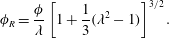 $$\begin{eqnarray}\displaystyle \unicode[STIX]{x1D719}_{R}=\frac{\unicode[STIX]{x1D719}}{\unicode[STIX]{x1D706}}\left[1+\frac{1}{3}(\unicode[STIX]{x1D706}^{2}-1)\right]^{3/2}. & & \displaystyle\end{eqnarray}$$
 The result for  $\boldsymbol{V}_{p}^{\prime \prime }$ for the spheroidal particles has the same form as that for a suspension of spheres in (2.24), except that the radius
  $b_{R}$ of the spheres must be found from (3.21).
4 Numerical calculation of two-particle interactions
Although far-field interactions and asymptotic results are sufficient to define a renormalization scheme, to obtain quantitative results it is necessary to evaluate  $\overline{\boldsymbol{W}}_{p}$ in (3.55). Hence, near-field interactions are required, and we calculate them by using a numerical version of the singularity method of Chwang & Wu (Reference Chwang and Wu1975, Reference Chwang and Wu1976). As first proposed by Dabros (Reference Dabros1985), we place point-force singularities inside the solid, spheroidal particles, and calculate their strengths by imposing the no-slip condition at points on their surfaces. A number of variations of this approach have been proposed for different problems governed by linear and even nonlinear equations. In the paragraphs below, we first describe our implementation of the singularity method, and then how the results are used to perform the integrations needed to obtain
  $\overline{\boldsymbol{W}}_{p}$.
4.1 Singularity method
In our implementation, we place  $N_{s}$ point-force singularities in each particle, arranged in circles centred on the axis of symmetry of the spheroidal particle. The singularities are a distance
  $\unicode[STIX]{x1D6FF}$ from the surface, in the direction of an inward pointing normal vector, as shown in figure 3. The circles are evenly spaced axially, except that one extra circle of singularities is located near the end of each particle, midway between the last regularly spaced circle and the particle tip, to more accurately capture the surface curvature there. The strengths
  $\boldsymbol{F}_{s}$ of the point-force singularities are determined by imposing no-slip conditions at
  $N_{s}$ points on the particle surfaces. Most calculations were done with 884 singularities in each particle (i.e. 21 circles of 42 singularities, with an additional singularity at the two ends). For
  $\unicode[STIX]{x1D706}=2.0$ and
  $\unicode[STIX]{x1D706}=3.0$, additional calculations were done with 580 singularities per particle, to verify numerical convergence.
In past work, it has been common to monitor the least-squares error in order to modify the magnitudes and placement of the singularities (Gotz Reference Gotz2005; Dabros Reference Dabros1985; Zhou & Pozrikidis Reference Zhou and Pozrikidis1995). However, particularly for far-field interactions between widely separated particles, adding singularities does not uniformly improve the accuracy of the method if optimized in this manner (Gotz Reference Gotz2005). In the current application, accurate calculation of far-field interactions is particularly important because, during integration, they are weighted by  $r^{2}$. Even an error of
  $10^{-3}$ can therefore become significant if, say,
  $r=6$. In the far-field limit for our sedimenting particles, the largest, slowest decaying interaction that remains after renormalization is the stresslet interaction described by (3.51). We found matching results to this result to be the most effective way to obtain the optimal separation distance
  $\unicode[STIX]{x1D6FF}$ between the singularities and the nearest point on the particle surface. In all cases, the separation was such that
  $0.045b\leqslant \unicode[STIX]{x1D6FF}\leqslant 0.23b$.

Figure 3. Schematic diagram of the two spheroidal particles with orientations  $\boldsymbol{d}_{0}$ and
  $\boldsymbol{d}_{1}$, respectively. The force applied to both particles is either
  $\boldsymbol{F}_{1}$ or
  $\boldsymbol{F}_{2}$. The vector
  $\boldsymbol{r}$, at angles
  $\unicode[STIX]{x1D6E9}$ and
  $\unicode[STIX]{x1D6F7}$ from
  $\boldsymbol{d}_{0}$, which is aligned with the
  $z$-axis, goes from the centre of the test particle to Particle 1. Point-force singularities are a distance
  $\unicode[STIX]{x1D6FF}$ from the surface, and are located in both particles, although only shown in Particle 2 for clarity.
To calculate sedimentation velocities, one must solve a ‘mobility problem’, in which the forces on the particles are specified and the particle velocities determined. In our singularity method, we therefore leave the particle translational velocities  $\boldsymbol{U}_{0}$ and
  $\boldsymbol{U}_{1}$ and rotational velocities
  $\unicode[STIX]{x1D734}_{0}$ and
  $\unicode[STIX]{x1D734}_{1}$ as unknown variables. The extra equations that are required come from the known, imposed force
  $\boldsymbol{F}$, equal for both particles, and the fact that the net torque on each particle is zero. Using the Oseen tensor from (2.15), the mathematical equations to be solved are
 $$\begin{eqnarray}\displaystyle \mathop{\sum }_{i=1}^{2N_{s}}\frac{1}{8\unicode[STIX]{x03C0}\unicode[STIX]{x1D702}}\unicode[STIX]{x1D645}(\boldsymbol{x}_{j}-\boldsymbol{x}_{s,i})\boldsymbol{\cdot }\boldsymbol{F}_{s,i}-\boldsymbol{U}_{p}-\unicode[STIX]{x1D734}_{p}\times (\boldsymbol{x}_{s,i}-\boldsymbol{x}_{p})=0, & & \displaystyle\end{eqnarray}$$
with
 $$\begin{eqnarray}\displaystyle \mathop{\sum }_{i=1}^{N_{s}}\boldsymbol{F}_{s,i}=\boldsymbol{F} & & \displaystyle\end{eqnarray}$$
and
 $$\begin{eqnarray}\displaystyle \mathop{\sum }_{i=1}^{N_{s}}(\boldsymbol{x}_{s,i}-\boldsymbol{x}_{p})\times \boldsymbol{F}_{s,i}=0. & & \displaystyle\end{eqnarray}$$
 Equation (4.1) is applied at  $N_{s}$ surface points
  $\boldsymbol{x}_{j}$ on each particle, and (4.2) and (4.3) provide the twelve (i.e. when applied to each particle) additional equations for the unknown particle translational and rotational velocities,
  $\boldsymbol{U}_{p}$ and
  $\unicode[STIX]{x1D734}_{p}$, respectively. Equations (4.1)–(4.3) are written for both particles. Hence, although for simplicity it is not reflected in the notation, there are two values of the particle velocities
  $\boldsymbol{U}_{p}$, rotational velocities
  $\unicode[STIX]{x1D734}_{p}$, and particle centres
  $\boldsymbol{x}_{p}$. Both particles are subject to the same force
  $\boldsymbol{F}$ in (4.2), and there is no applied torque acting on either particle, so that the right side of (4.3) is zero. Equations (4.1)–(4.3) form a set of linear equations that were solved by standard methods (Press et al. Reference Press, Flannery, Teukolsky and Vetterling1989) to obtain the singularity strengths
  $\boldsymbol{F}_{s}$, particle velocities
  $\boldsymbol{U}_{p}$ and rotational velocities
  $\unicode[STIX]{x1D734}_{p}$.

Figure 4. Normalized sedimentation velocity  $U_{z}$ of two particles subjected to a force
  $-F\boldsymbol{e}_{z}$ in (a) axisymmetric (i.e.
  $\boldsymbol{x}_{1}-\boldsymbol{x}_{0}=s\boldsymbol{e}_{z}$,
  $\boldsymbol{d}_{0}=\boldsymbol{d}_{1}=\boldsymbol{e}_{z}$) and (b) side by side (i.e.
  $\boldsymbol{x}_{1}-\boldsymbol{x}_{0}=s\boldsymbol{e}_{x}$,
  $\boldsymbol{d}_{0}=\boldsymbol{d}_{1}=\boldsymbol{e}_{y}$) configurations. Solid dots are from the singularity method,
  $\times$ symbols (blue) are two-sphere results (Stimson & Jeffery Reference Stimson and Jeffery1926; Goldman et al. Reference Goldman, Cox and Brenner1966; Batchelor Reference Batchelor1972),
  $+$ symbols are collocation results (Gluckman et al. Reference Gluckman, Pfeffer and Weinbaum1971) and solid curves (red) are first-reflection results (Kim Reference Kim1985).
Results for particle velocities calculated from (4.1)–(4.3) are shown in figure 4(a,b). Two different two-particle configurations are considered. In figure 4(a), the axis of symmetry of each particle (i.e. the direction of  $\boldsymbol{d}_{0}$ and
  $\boldsymbol{d}_{1}$) is in the
  $z$ direction, the two particles are separated by a distance
  $s\boldsymbol{e}_{z}$, and the applied force is
  $F\boldsymbol{e}_{z}$. The problem is therefore axisymmetric. Results from the singularity method used here agree quantitatively both with the exact two-sphere results of Stimson & Jeffery (Reference Stimson and Jeffery1926) when
  $\unicode[STIX]{x1D706}=1.0001$, and with the collocation results of Gluckman et al. (Reference Gluckman, Pfeffer and Weinbaum1971) when
  $\unicode[STIX]{x1D706}=2$.
In figure 4(b), the applied force is unchanged but the particles are separated in the  $x$-direction and
  $\boldsymbol{d}_{0}$ and
  $\boldsymbol{d}_{1}$ point in the
  $y$-direction. The singularity calculation again shows quantitative agreement with exact two-sphere results (Goldman et al. Reference Goldman, Cox and Brenner1966), except when
  $s<2.0049a$, when lubrication interactions between the rotating particles cause a slight,
  $1.6\,\%$ decrease in the sedimentation velocity (see e.g. table 1 in Batchelor (Reference Batchelor1972)) that is not reproduced numerically. However, the range of that interaction is so small that it has a negligible effect on the final result for the sedimentation velocity. In both figures 4(a) and 4(b), far-field or ‘first-reflection’ results are shown as derived by Kim (Reference Kim1985), and they are in quantitative agreement with our numerical calculations as the particle separation increases.
4.2 Numerical integration
To compute  $\overline{\boldsymbol{W}}_{p}$ in (3.55) using the two-particle solution, we must integrate over all orientations of both particles, as well as the particle–particle separation
  $\boldsymbol{r}$. However, because of the linearity of the governing equations, the velocity of the test particle at any orientation
  $\unicode[STIX]{x1D6FA}_{0}$, after averaging over positions and orientations of the second particle, can be expressed a superposition of motion along the particle axis
  $\boldsymbol{d}_{0}$ and perpendicular to it. We therefore obtain
  $\overline{\boldsymbol{W}}_{p}$ as an orientation average over two problems. In the first, the imposed force (
 $\boldsymbol{F}_{1}$ in figure 3) on both particles is parallel to
  $\boldsymbol{d}_{0}$, and all possible orientations and positions of the second particle are integrated explicitly. This geometry is axisymmetric about the axis of the test particle, so that the integration over
  $\unicode[STIX]{x1D6F7}$ in figure 3 is trivial. In the second problem, the imposed force (
 $\boldsymbol{F}_{2}$ in figure 3) on both particles is perpendicular to
  $\boldsymbol{d}_{0}$, and integration over
  $\unicode[STIX]{x1D6F7}$ must be done explicitly.
The complete, orientation-averaged mobility of the test particle is obtained using results from these two directions. Just as in (3.12), one third of the complete result is contributed by the axisymmetric problem in which the imposed force is  $\boldsymbol{F}_{1}$, and two thirds from the problem in which the imposed force is
  $\boldsymbol{F}_{2}$. If we use angle brackets to describe the average effect of the second particle (Particle 1) on the motion of the test particle, before averaging over orientation of the test particle, with subscripts
  $i=1$ or
  $i=2$ to indicate the case where the imposed force is
  $\boldsymbol{F}_{1}$ or
  $\boldsymbol{F}_{2}$, then
 $$\begin{eqnarray}\displaystyle \langle \boldsymbol{W}_{p,i}\rangle =\int _{\boldsymbol{r}}\int _{\unicode[STIX]{x1D6FA}_{1}}\boldsymbol{W}_{p,i}(\boldsymbol{x}_{0},\unicode[STIX]{x1D6FA}_{0},\boldsymbol{x}_{0}+\boldsymbol{r},\unicode[STIX]{x1D6FA}_{1})P_{p}(\boldsymbol{x}_{0}+\boldsymbol{r},\unicode[STIX]{x1D6FA}_{1}|\boldsymbol{x}_{0},\unicode[STIX]{x1D6FA}_{0})\,\text{d}\unicode[STIX]{x1D6FA}_{1}\,\text{d}\boldsymbol{r} & & \displaystyle\end{eqnarray}$$
and
 $$\begin{eqnarray}\displaystyle \overline{\boldsymbol{W}}_{p}=\frac{\langle \boldsymbol{W}_{p,1}\rangle }{3}+\frac{2\langle \boldsymbol{W}_{p,2}\rangle }{3}. & & \displaystyle\end{eqnarray}$$
 The integrals in (4.4) must be calculated separately for the axisymmetric and non-axisymmetric cases. There are at most five integrations required. The particle orientation  $\unicode[STIX]{x1D6FA}_{1}$ may be specified by two angles
  $(\unicode[STIX]{x1D703}_{1},\unicode[STIX]{x1D719}_{1})$, and the integration over
  $\boldsymbol{r}$ requires integration over the separation distance
  $r$, as well as the two angles
  $(\unicode[STIX]{x1D6E9},\unicode[STIX]{x1D6F7})$ that are defined by the relative positions of the particle centres at
  $\boldsymbol{x}_{0}$ and
  $\boldsymbol{x}_{1}$ (cf. figure 3). For the axisymmetric problem, the integration over
  $\unicode[STIX]{x1D6F7}$ is trivial, as stated above.
We integrate over orientations  $\unicode[STIX]{x1D6FA}_{1}$ or, equivalently,
  $(\unicode[STIX]{x1D703}_{1},\unicode[STIX]{x1D719}_{1})$ by using Lebedev quadrature (Levedev & Laikov Reference Levedev and Laikov1999; Gross & Atzberger Reference Gross and Atzberger2018). Lebedev quadrature is comparable to Gauss quadrature in two dimensions, but is more efficient over the surface of a unit sphere because it avoids a congregation of Gauss points at the poles (cf. figure 2 in Gross & Atzberger (Reference Gross and Atzberger2018)). Lebedev quadrature is described by Abramowitz & Stegun (Reference Abramowitz and Stegun1972), although they do not use that name, and rather group it with other Gauss quadrature schemes. Our integration was done with 26 and 38 orientations, with the larger value used to verify convergence. However, in practice only half of the orientations over a unit sphere need to be considered. For our symmetric, spheroidal particles, a 26 point Lebedev quadrature requires only 13 orientations, because a particle with orientation
  $\boldsymbol{d}_{1}$ is indistinguishable from a particle with orientation
  $-\boldsymbol{d}_{1}$.
For each orientation  $(\unicode[STIX]{x1D703}_{1},\unicode[STIX]{x1D719}_{1})$ and separation direction
  $(\unicode[STIX]{x1D6E9},\unicode[STIX]{x1D6F7})$, the minimum separation
  $r=|\boldsymbol{r}|$ at contact,
  $r_{lim}(\unicode[STIX]{x1D703}_{1},\unicode[STIX]{x1D719}_{1},\unicode[STIX]{x1D6E9},\unicode[STIX]{x1D6F7})$, was found by locating the point of particle contact along the line between particle centres defined by
  $(\unicode[STIX]{x1D6E9},\unicode[STIX]{x1D6F7})$. Then the numerical integration over possible centre positions
  $\boldsymbol{r}$ was done over
  $r_{lim}\leqslant r\leqslant 6a$,
  $0\leqslant \unicode[STIX]{x1D6E9}\leqslant \unicode[STIX]{x03C0}$ and, when required,
  $0\leqslant \unicode[STIX]{x1D6F7}\leqslant 2\unicode[STIX]{x03C0}$. The integration over
  $r$ was done in sections, from
  $r_{lim}\leqslant r<3a$,
  $3a\leqslant r\leqslant 4a$,
  $4a\leqslant r\leqslant 5a$ and
  $5a\leqslant r\leqslant 6a$, by 10 point Gauss quadrature in each section. The integrations over
  $\unicode[STIX]{x1D6E9}$ and
  $\unicode[STIX]{x1D6F7}$ (where required) were done by Gauss quadrature with
  $N_{\unicode[STIX]{x1D6E9}}=N_{\unicode[STIX]{x1D6F7}}=10$ points, respectively. Convergence was verified assessed in all cases by increasing the number of Gauss points from 10 to 20. Integration from
  $r=6a$ to
  $r\rightarrow \infty$ was done using the asymptotic, orientation-averaged second-reflection interaction given in (3.50). Transitioning to the asymptotic result at a separation of
  $6a$ rather than the
  $8a$ used by Batchelor (Reference Batchelor1972) was sufficient because the interactions decay faster for spheroidal particles than for spheres (see e.g. figure 4).
If the right side of (4.4) is expressed in dimensionless form, the contributions  $\langle \boldsymbol{W}_{p,i}\rangle$ may be expressed as
 $$\begin{eqnarray}\displaystyle \langle \boldsymbol{W}_{p,i}\rangle =\frac{\boldsymbol{F}_{i}}{6\unicode[STIX]{x03C0}\unicode[STIX]{x1D707}a}\unicode[STIX]{x1D719}\unicode[STIX]{x1D706}^{2}\frac{3}{4\unicode[STIX]{x03C0}}\widehat{U}_{c,i}, & & \displaystyle\end{eqnarray}$$
where
 $$\begin{eqnarray}\displaystyle \widehat{U}_{c,i}=\int _{\hat{\boldsymbol{r}}}\int _{\unicode[STIX]{x1D6FA}_{1}}\widehat{W}_{p,i}\hat{P}_{p}\,\text{d}\unicode[STIX]{x1D6FA}_{1}\,\text{d}\hat{\boldsymbol{r}}. & & \displaystyle\end{eqnarray}$$
In (4.7),
 $$\begin{eqnarray}\displaystyle \widehat{W}_{p,i}=|\boldsymbol{W}_{p,i}|\frac{6\unicode[STIX]{x03C0}\unicode[STIX]{x1D702}a}{|\boldsymbol{F}|} & & \displaystyle\end{eqnarray}$$
 and  $\hat{P}_{p}$ has been normalized by the number density
  $n$. Consistent with (4.5), we define
  $\widehat{U}_{c}$ as
 $$\begin{eqnarray}\displaystyle \widehat{U}_{c}=\widehat{U}_{c}^{N}+\widehat{U}_{c}^{\infty }, & & \displaystyle\end{eqnarray}$$
where
 $$\begin{eqnarray}\displaystyle \widehat{U}_{c}^{N}=\frac{\widehat{U}_{c,1}^{N}}{3}+\frac{2\widehat{U}_{c,2}^{N}}{3}, & & \displaystyle\end{eqnarray}$$
 the superscript ‘ $N$’ indicates a near-field, numerical result for separations
  $r_{lim}\leqslant r\leqslant 6a$, and the superscript
  $\infty$ denotes the contribution from
  $r>6a$. In (4.6), (3.7) has been used to convert the number density
  $n$ to volume fraction
  $\unicode[STIX]{x1D719}$. Numerical results for
  $\widehat{U}_{c}^{N}$ are given in table 4.
Table 4. Values of  $\widehat{U}_{c}$.

To derive a complete result for the particle flux caused by the thermodynamic force in (2.1), we combine the  $O(\unicode[STIX]{x1D719})$ contributions from (3.64), (3.69), (4.6)–(4.9), the single-spheroid result from (3.12), and use (3.22) and (3.23). Defining a mobility factor
  $\unicode[STIX]{x1D709}_{m}$ for the spheroidal particles as
 $$\begin{eqnarray}\displaystyle \unicode[STIX]{x1D709}_{m}=\frac{1}{3}\left[\frac{1}{X_{A}}+\frac{2}{Y_{A}}\right], & & \displaystyle\end{eqnarray}$$
 we then find for the volume flux  $\overline{\boldsymbol{U}}\unicode[STIX]{x1D719}$:
 $$\begin{eqnarray}\displaystyle \overline{\boldsymbol{U}}\unicode[STIX]{x1D719} & = & \displaystyle -\unicode[STIX]{x1D709}_{m}D_{0}(1+2B_{2}\unicode[STIX]{x1D719})\nonumber\\ \displaystyle & & \displaystyle \times \left\{1-\frac{\unicode[STIX]{x1D719}}{\hat{b}_{R}\unicode[STIX]{x1D709}_{m}}\left[\frac{1}{\unicode[STIX]{x1D706}}+3\unicode[STIX]{x1D706}^{2}I_{1}+3\unicode[STIX]{x1D706}^{2}\hat{b}_{R}I_{2}\right]+\unicode[STIX]{x1D719}\frac{\unicode[STIX]{x1D706}^{2}\hat{b}_{R}^{2}}{2\unicode[STIX]{x1D709}_{m}}+\frac{3\unicode[STIX]{x1D706}^{2}\unicode[STIX]{x1D719}}{4\unicode[STIX]{x03C0}\unicode[STIX]{x1D709}_{m}}\widehat{U}_{c}\right\}\unicode[STIX]{x1D735}\unicode[STIX]{x1D719}.\end{eqnarray}$$
 Here,  $D_{0}$ is the result given in (2.7), except that the dimension
  $a$ is the half-length of the long axis of the particle rather than a sphere radius. The product
  $\unicode[STIX]{x1D709}_{m}D_{0}$, where
  $\unicode[STIX]{x1D709}_{m}\geqslant 1$, is the Stokes–Einstein diffusivity with the mobility changed to reflect the spheroidal nature of the particle, which has a higher mobility than a sphere with radius
  $a$.
$a$.
4.3 The diffusivity to O( $\unicode[STIX]{x1D719}$)

The term on the right side of (4.12) is the concentration-dependent diffusion coefficient  $D(\unicode[STIX]{x1D719},\unicode[STIX]{x1D706})$ multiplied by
  $-\unicode[STIX]{x1D735}\unicode[STIX]{x1D719}$. To
  $O(\unicode[STIX]{x1D719})$, then,
 $$\begin{eqnarray}\displaystyle & \displaystyle D(\unicode[STIX]{x1D719},\unicode[STIX]{x1D706})=\unicode[STIX]{x1D709}_{m}D_{0}(1+D_{1}\unicode[STIX]{x1D719}), & \displaystyle\end{eqnarray}$$
 $$\begin{eqnarray}\displaystyle & \displaystyle D_{1}=2B_{2}-K_{f} & \displaystyle\end{eqnarray}$$
and
 $$\begin{eqnarray}\displaystyle K_{f}=\frac{1}{\hat{b}_{R}\unicode[STIX]{x1D709}_{m}}\left[\frac{1}{\unicode[STIX]{x1D706}}+3\unicode[STIX]{x1D706}^{2}I_{1}+3\unicode[STIX]{x1D706}^{2}\hat{b}_{R}I_{2}\right]-\frac{\unicode[STIX]{x1D706}^{2}\hat{b}_{R}^{2}}{2\unicode[STIX]{x1D709}_{m}}-\frac{3\unicode[STIX]{x1D706}^{2}}{4\unicode[STIX]{x03C0}\unicode[STIX]{x1D709}_{m}}\widehat{U}_{c}. & & \displaystyle\end{eqnarray}$$
 For spherical particles,  $\unicode[STIX]{x1D709}_{m}=1$,
  $\unicode[STIX]{x1D706}=1$,
  $\hat{b}_{R}=1$,
  $I_{1}=0$,
  $I_{2}=3/2$,
  $B_{2}=4$ and
  $3\widehat{U}_{c}/4\unicode[STIX]{x03C0}=-1.55$, so that to
  $O(\unicode[STIX]{x1D719})$ the gradient diffusion coefficient is
  $D_{0}(1+1.45\unicode[STIX]{x1D719})$. Values of
  $D_{1}$ for
  $1\leqslant \unicode[STIX]{x1D706}\leqslant 3.5$ are given in table 5.
Table 5. Values of  $K_{f}$ and
  $D_{1}$.

Dogic et al. (Reference Dogic, Philipse, Fraden and Dhont2000) and Peterson (Reference Peterson1964) have calculated sedimentation rates for long rods, for which  $\unicode[STIX]{x1D706}\gg 1$. Dogic et al. (Reference Dogic, Philipse, Fraden and Dhont2000), in particular, use Batchelor’s renormalization method, and obtain the result that to
  $O(1/\unicode[STIX]{x1D706})$
 $$\begin{eqnarray}\displaystyle K_{f,rod}=\frac{6.4+(2/9)\unicode[STIX]{x1D706}}{2\ln \unicode[STIX]{x1D706}+0.63}\unicode[STIX]{x1D706}. & & \displaystyle\end{eqnarray}$$
 At  $\unicode[STIX]{x1D706}=3$ and
  $\unicode[STIX]{x1D706}=3.5$, (4.16) yields
  $K_{f,rod}=7.5$ and
  $K_{f,rod}=8.0$, respectively. Considering that the results derived here are for spheroidal particles, not long rods, these values are in reasonable agreement with those in table 5. With the second virial coefficient
  $B_{2}$, equation (4.16) could be used to predict the value of
  $D_{1}$ at higher aspect ratios than
  $\unicode[STIX]{x1D706}=3.5$. However, the two-particle calculation used here is subject to the constraint that
  $\unicode[STIX]{x1D719}\unicode[STIX]{x1D706}^{2}\ll 1$, making it unlikely that predictions for
  $D_{1}$ at higher values or
  $\unicode[STIX]{x1D706}>3.5$ could be observed in experiments.
The results for  $D(\unicode[STIX]{x1D719},\unicode[STIX]{x1D706})$ predicted from table 5 may be conveniently calculated by means of the correlation
 $$\begin{eqnarray}\displaystyle D(\unicode[STIX]{x1D719},\unicode[STIX]{x1D706})=\unicode[STIX]{x1D709}_{m}D_{0}[1+1.45\unicode[STIX]{x1D719}[1+0.259(\unicode[STIX]{x1D706}-1)+0.126(\unicode[STIX]{x1D706}-1)^{2}]]. & & \displaystyle\end{eqnarray}$$
 Equation (4.17) reproduces the results in table 5 to within  $1\,\%$, with the exception of the result at
  $\unicode[STIX]{x1D706}=1.25$. That result falls approximately
  $4\,\%$ below the correlation prediction, a difference that appears to be caused by the relatively modest increase in
  $B_{2}$ between
  $\unicode[STIX]{x1D706}=1.0$ and
  $\unicode[STIX]{x1D706}=1.25$, both in our calculations and those of Mulder & Frenkel (Reference Mulder and Frenkel1985), as shown in table 1.
5 Diffusion of bovine serum albumin
Although globular proteins are typically not hard spheres or hard spheroids, and undergo non-hydrodynamic interactions, there is a long history of making inferences about the nature of their interactions by comparing diffusion data with theoretical predictions. As mentioned in the Introduction, bovine serum albumin (BSA) is a protein that was for many years described as being, approximately, a prolate spheroid with  $\unicode[STIX]{x1D706}=3.5$ (Squire et al. Reference Squire, Moser and O’Konski1968; Wright & Thompson Reference Wright and Thompson1975). For example, Wright & Thompson (Reference Wright and Thompson1975) give the dimensions as
  $2a=14.1\pm 0.5~\text{nm}$ and
  $2b=4.2\pm 0.4~\text{nm}$. More recently a smaller aspect ratio
  $\unicode[STIX]{x1D706}=1.9$ was proposed (Jachimska et al. Reference Jachimska, Wasilewska and Adamczyk2008), and the prolate shape itself has been questioned (Carter & Ho Reference Carter and Ho1994; Ferrer et al. Reference Ferrer, Duchowicz, Carrasco, de la Torre and Acuna2001; Leggio et al. Reference Leggio, Galantini and Pavel2008). It is therefore of interest to compare measurements from static and dynamic light scattering with predictions from virial expansions and diffusivities for hard, spheroidal particles with different aspect ratios.

Figure 5. Reduced light-scattering intensities  $KCM/R_{\unicode[STIX]{x1D703}}$ for BSA solutions from Meechai, Jamieson & Blackwell (Reference Meechai, Jamieson and Blackwell1999), plotted versus volume fraction
  $\unicode[STIX]{x1D719}$. Experimental data in blue correspond to the isoelectric point
  $\text{pH}=4.7$,
  $I=0.1$; in red to the conditions
  $\text{pH}=7.4$,
  $I=1.5$; and in black to the conditions
  $\text{pH}=7.4$,
  $I=0.15$. Solid and dashed curves are predictions from the hard-spheroid virial expansions for
  $\unicode[STIX]{x1D706}=3.5$ and
  $\unicode[STIX]{x1D706}=1.9$, respectively.
To this end we make use of the experimental results of Meechai et al. (Reference Meechai, Jamieson and Blackwell1999), who report light-scattering results for three different BSA solutions at different pH levels and ionic strengths. The solutions are (i) at the isoelectric point,  $\text{pH}=4.7$ and ionic strength
  $I=0.1$; (ii) at
  $\text{pH}=7.4$ and ionic strength
  $I=1.5$; and (iii) at
  $\text{pH}=7.4$ and ionic strength
  $I=0.15$. The corresponding Debye screening lengths for the two cases where the BSA is charged are 0.25 nm and 0.8 nm for
  $I=1.5$ and
  $I=0.15$, respectively. In their paper, Meechai et al. (Reference Meechai, Jamieson and Blackwell1999) compare reduced light scattering intensities
  $KCM/R_{\unicode[STIX]{x1D703}}$ with the prediction from the virial expansion for hard spheres, as given by (2.8), except that Meechai et al. (Reference Meechai, Jamieson and Blackwell1999) include contributions from the third and fourth virial coefficients. In the reduced scattering intensity,
  $K$ is an optical constant,
  $C$ is the BSA concentration expressed as mass per unit volume,
  $M$ is the molecular weight of the BSA, and
  $R_{\unicode[STIX]{x1D703}}$ is the Rayleigh ratio. Values for these parameters are given in the paper by Meechai et al. (Reference Meechai, Jamieson and Blackwell1999).
In figure 5, the reduced scattering intensities for BSA solutions measured by Meechai et al. (Reference Meechai, Jamieson and Blackwell1999) are plotted, with predictions from virial expansions for hard spheroidal BSA molecules instead of hard spheres. The scattering intensities are related to the virial expansions by (Selim et al. Reference Selim, Al-Naafa and Jones1993; Meechai et al. Reference Meechai, Jamieson and Blackwell1999)
 $$\begin{eqnarray}\displaystyle \frac{KCM}{R_{\unicode[STIX]{x1D703}}}=\frac{1}{kT}\left(\frac{\unicode[STIX]{x2202}\unicode[STIX]{x03C0}}{\unicode[STIX]{x2202}n}\right)_{P,T}=1+2B_{2}(\unicode[STIX]{x1D706})\unicode[STIX]{x1D719}+3B_{3}(\unicode[STIX]{x1D706})\unicode[STIX]{x1D719}^{2}+\cdots & & \displaystyle\end{eqnarray}$$
 The fourth virial coefficients for spheres are included by Meechai et al. (Reference Meechai, Jamieson and Blackwell1999), but are not available for prolate spheroidal solutes. The second and third coefficients for hard spheroids can be found from table 1 in § 3.2 and by interpolation from table 1 in the paper by Mulder & Frenkel (Reference Mulder and Frenkel1985). The dashed curve in figure 5 corresponds to  $\unicode[STIX]{x1D706}=1.9$ as proposed in Jachimska et al. (Reference Jachimska, Wasilewska and Adamczyk2008), and the solid curve corresponds to
  $\unicode[STIX]{x1D706}=3.5$. The values of
  $B_{2}$ and
  $B_{3}$ are 4.47 and 11.84 for
  $\unicode[STIX]{x1D706}=1.9$, and 5.96 and 18.2 for
  $\unicode[STIX]{x1D706}=3.5$.

Figure 6. Normalized gradient diffusion coefficients  $D/D_{0}$ for BSA solutions from Meechai et al. (Reference Meechai, Jamieson and Blackwell1999), plotted versus volume fraction
  $\unicode[STIX]{x1D719}$. Experimental data in blue correspond to the isoelectric point
  $\text{pH}=4.7$,
  $I=0.1$; in red to the conditions
  $\text{pH}=7.4$,
  $I=1.5$; and in black to the conditions
  $\text{pH}=7.4$,
  $I=0.15$. Solid and dashed curves are predictions from (4.17) for
  $\unicode[STIX]{x1D706}=3.5$ and
  $\unicode[STIX]{x1D706}=1.9$, respectively.
Both virial expansions are well above the measurements for BSA at its isoelectric point, indicating an attraction between uncharged BSA molecules. The plots for  $\unicode[STIX]{x1D706}=1.9$ and
  $\unicode[STIX]{x1D706}=3.5$ lie close to, but slightly below, the data for BSA solutions at
  $\text{pH}=7.4$ and
  $I=1.5$ and
  $I=0.15$, respectively. It is noteworthy that the contribution from the fourth virial term is almost certainly not negligible over the range of volume fraction shown. The fourth virial coefficient for hard spheres is 18, yielding a contribution of
  $72\unicode[STIX]{x1D719}^{3}$. The second and third virial coefficients for spheroids are both significantly larger than their counterparts for hard spheres, and it seems likely the same would be true for the fourth coefficient. Including a contribution
  $4B_{4}\unicode[STIX]{x1D719}^{3}$ would slightly raise the positions of both the solid and dashed curves in figure 5. The virial expansion for
  $\unicode[STIX]{x1D706}=1.9$ may therefore be considered to be in reasonable agreement with the experimental data corresponding to
  $\text{pH}=7.4$ and
  $I=1.5$; the virial expansion for
  $\unicode[STIX]{x1D706}=3.5$ may similarly be considered to be in reasonable agreement with the data for
  $\text{pH}=7.4$ and
  $I=0.15$.
The gradient diffusion coefficients corresponding to the three cases, as reported by Meechai et al. (Reference Meechai, Jamieson and Blackwell1999), are plotted in figure 6, along with the prediction of (4.17). The experimental data for BSA solutions at the isoelectric point decrease with increasing concentration, which is consistent with the presence of an attraction, as inferred from figure 5. Meechai et al. (Reference Meechai, Jamieson and Blackwell1999) also conclude a long-range attraction is present at those conditions. The predictions from (4.17), for both  $\unicode[STIX]{x1D706}=1.9$ and
  $\unicode[STIX]{x1D706}=3.5$, are in proximity to the diffusivities measured at
  $\text{pH}=7.4$ and
  $I=0.15$. The higher ionic strength of
  $I=1.5$, corresponding to a Debye screening length of only 0.25 nm, comparable to the diameter of a water molecule, is apparently insufficient to counteract the attractive interaction. The fact that the higher aspect ratio of
  $\unicode[STIX]{x1D706}=3.5$ yields good agreement between theory and experiment for hard spheroids, both for the virial expansions and diffusion coefficients, supports the contention that BSA behaves hydrodynamically as a hard spheroid with the larger aspect ratio, at
  $\text{pH}=7.4$ and
  $I=0.15$.
6 Conclusion
The shape of a diffusing colloidal particle modifies the concentration dependence of its collective, or gradient, diffusion coefficient. Hence, efforts at interpretation of that concentration dependence without accounting for a non-spherical shape can be misleading. For hard spheroidal particles, it is shown here that both the second virial coefficient and sedimentation coefficient increase with the particle aspect ratio. However, for modest aspect ratios, the increase in the virial coefficient is greater, leading to an increase in the concentration dependence of the gradient diffusion coefficient. When the aspect ratio of the spheroid is increased from 1 to 3.5, the coefficient  $D_{1}$ describing the concentration dependence increases by a factor of approximately 2.4. Even when a diffusing macromolecule or colloidal particle is not a hard spheroid, comparison with these predictions can yield useful information.
Acknowledgements
This research was funded by a grant from the National Science Foundation (CBET 1506474). The author gratefully acknowledges helpful conversations with S. R. Dungan and N. P. Alexander. Our collaborative study of diffusion in micelle solutions led to the questions that inspired this work.


 Open access