


1 Background
Shock buffet on wings is an undesirable phenomenon limiting the flight envelope at high Mach numbers and load factors. Its study is critical for commercial transonic air transport. The term shock buffet refers to an aerodynamic instability with self-sustained shock-wave oscillations and intermittent boundary-layer separation. Whereas aerofoil buffet in fully turbulent flow is characterised by large chordwise shock excursions at dominant Strouhal numbers (i.e. dimensionless frequency of oscillation using mean aerodynamic chord and free-stream speed) of 0.06 to 0.07, well-developed wing buffet typically comes with lower-amplitude shock motions and is more broadband with up to an order of magnitude higher frequencies (Strouhal numbers of 0.2 to 0.6) depending e.g. on sweep angle (Dandois Reference Dandois2016). A spanwise outboard propagation of buffet cells (a term coined by Iovnovich & Raveh (Reference Iovnovich and Raveh2015)), which is believed to constitute the instability, has been reported both in experimental and numerical studies (Lawson, Greenwell & Quinn Reference Lawson, Greenwell and Quinn2016; Sartor & Timme Reference Sartor and Timme2017; Sugioka et al. Reference Sugioka, Koike, Nakakita, Numata, Nonomura and Asai2018). A spanwise inboard propagation, dominant along the shock front, has also been identified experimentally at lower frequencies (Dandois Reference Dandois2016; Masini et al. Reference Masini, Timme, Ciarella and Peace2017; Masini, Timme & Peace Reference Masini, Timme and Peace2020). Timme & Thormann (Reference Timme and Thormann2016) observed resonant flow due to forced wing vibration in the same lower frequency range, in addition to distinct flow responses around typical shock-buffet frequencies on wings. While the flow unsteadiness is self-excited, not requiring structural vibration itself (Steimle, Karhoff & Schröder Reference Steimle, Karhoff and Schröder2012), resulting aerodynamic loads excite the wing structure (called buffeting) thus deteriorating passenger comfort, flight control and performance and the fatigue life. Certification specifications stipulate that an aircraft must be free of any vibration and buffeting in cruising flight with a margin of  $0.3g$ (where
  $g$ is the gravitational acceleration) to the buffet onset boundary.
Shock-buffet characteristics on aerofoils and wings are distinct, and despite more than half a century of research an unequivocally agreed physical interpretation is still debated (Giannelis, Vio & Levinski Reference Giannelis, Vio and Levinski2017). An important theoretical/numerical advance was the Crouch, Garbaruk & Magidov (Reference Crouch, Garbaruk and Magidov2007), Crouch et al. (Reference Crouch, Garbaruk, Magidov and Travin2009) discovery of a global (asymptotic, modal, absolute) instability leading to aerofoil buffet, using Reynolds-averaged Navier–Stokes (RANS) aerodynamics in a base-flow scenario. The interested reader is referred to the excellent reviews by Sipp et al. (Reference Sipp, Marquet, Meliga and Barbagallo2010) and Theofilis (Reference Theofilis2011) for a reflection on the various terms denoting such oscillator-type flow instability resulting from a Hopf bifurcation. A base-flow approach essentially refers to linearising both the RANS equations and a turbulence model around an equilibrium point (i.e. a steady-state solution) (Mettot, Sipp & Bézard Reference Mettot, Sipp and Bézard2014). Even though Crouch’s description of the instability somewhat differs from the widely discussed model by Lee (Reference Lee1990), the two models both rely on an acoustic feedback mechanism and involvement of the trailing edge, an observation which is also supported by eddy-resolving simulation (e.g. Deck Reference Deck2005; Grossi, Braza & Hoarau Reference Grossi, Braza and Hoarau2014) and experiment (e.g. Hartmann, Feldhusen & Schröder Reference Hartmann, Feldhusen and Schröder2013; Feldhusen–Hoffmann et al. Reference Feldhusen–Hoffmann, Statnikov, Michael and Schröder2018). Reconciliation of a universal aerofoil buffet model is desirable. Sartor, Mettot & Sipp (Reference Sartor, Mettot and Sipp2015) additionally identified a convective medium-frequency Kelvin–Helmholtz-type instability via optimal-forcing responses using the resolvent approach. In the three-dimensional case, Iovnovich & Raveh (Reference Iovnovich and Raveh2015) pursued the categorisation of the three-dimensionality of wing buffet by progressively building up the geometric complexity. Similarly, relying on a basic infinite-wing set-up, the isolated impact of sweep angle has been studied using modal analysis (Crouch, Garbaruk & Strelet Reference Crouch, Garbaruk and Strelet2019; Paladini et al. Reference Paladini, Beneddine, Dandois, Sipp and Robinet2019a; Plante et al. Reference Plante, Dandois, Beneddine, Sipp and Laurendeau2019a) and time-marching unsteady RANS (Plante, Dandois & Laurendeau Reference Plante, Dandois and Laurendeau2019b). Scale-resolving detached-eddy simulation on the other hand has been applied for finite-wing shock-buffet flow by Brunet & Deck (Reference Brunet and Deck2008), Sartor & Timme (Reference Sartor and Timme2017) and Ohmichi, Ishida & Hashimoto (Reference Ohmichi, Ishida and Hashimoto2018), supporting the above mentioned spanwise propagation of buffet cells. At the same time, industrial practice mostly relies on steady RANS analysis e.g. with the ‘ $\unicode[STIX]{x0394}\unicode[STIX]{x1D6FC}=0.1^{\circ }$ offset’ method (where
  $\unicode[STIX]{x1D6FC}$ is the angle of attack) to decide on shock-buffet onset (Lawson et al. Reference Lawson, Greenwell and Quinn2016).
In recent years, modal descriptions of shock buffet on finite wings have been pursued intensively. Ohmichi et al. (Reference Ohmichi, Ishida and Hashimoto2018) applied modal identification techniques, specifically proper orthogonal decomposition and dynamic mode decomposition, to discern dominant modal aerodynamic behaviour from solution snapshots well beyond buffet onset. Focussing instead on the discretised RANS (plus turbulence model) operator directly, global mode computation on a case with three inhomogeneous spatial dimensions has first been accomplished in pre-buffet conditions by Timme & Thormann (Reference Timme and Thormann2016), for the experiment described in Lawson et al. (Reference Lawson, Greenwell and Quinn2016) and Masini et al. (Reference Masini, Timme, Ciarella and Peace2017, Reference Masini, Timme and Peace2020). Although not the first reported proper three-dimensional stability analysis (see Theofilis (Reference Theofilis2011) for a short, yet quickly growing list), the work focussed exclusively on geometric non-canonical complexity and flow parameters, specifically high Reynolds number, relevant to an aircraft wing. A conclusive identification of the sought unstable global mode, with the chosen numerical approach, failed due to non-converging base flow in the vicinity of suspected buffet onset, and this would require, for instance, a matrix-free time-stepping iterative tool for modal analysis (see for example Eriksson & Rizzi (Reference Eriksson and Rizzi1985) and Barkley, Blackburn & Sherwin (Reference Barkley, Blackburn and Sherwin2008)).
Previous aerofoil buffet studies using global stability theory applied sparse direct linear equation solvers with a full factorisation of the coefficient matrix. The bottleneck is the excessive memory requirement that has already been observed for simple aerofoil cases (Iorio, Gonzalez & Ferrer Reference Iorio, Gonzalez and Ferrer2014). This renders direct methods infeasible for truly three-dimensional cases, when solving linear systems arising from a shift-and-invert approach, used for instance in the implicitly restarted Arnoldi method (Sorensen Reference Sorensen1992). A viable alternative is to use sparse iterative linear equation solvers, and the generalised minimal residual method (Saad & Schultz Reference Saad and Schultz1986) has become standard practice. Trading memory requirements for computing time, such iterative methods often stall for very stiff problems, as found in transonic turbulent flow near buffet onset and exacerbated by the nearly singular shift-and-invert preconditioned matrix eigenvalue problem. Timme & Thormann (Reference Timme and Thormann2016) opted for a Krylov method with deflated restarting to make their tools robust.
An important, and currently missing, link in the fundamental understanding of the very basics of three-dimensional shock buffet on finite wings, analogous to the seminal aerofoil work by Crouch et al. (Reference Crouch, Garbaruk and Magidov2007, Reference Crouch, Garbaruk, Magidov and Travin2009), is confirmation of the existence of an unstable global mode, or even multiple modes indeed. This is the central question to be addressed in this work. Section 2 introduces the numerical approach, followed by § 3 outlining the chosen test case and some basic validation of the simulations. Details of the physically relevant modes, placing emphasis on the dominant unstable global mode describing the incipient shock-buffet instability and its relation to the saturated nonlinear response, are presented in § 4. Convergence studies relating to the mesh and chosen iterative methods are provided in the appendices.
2 Numerical approach
The aerodynamics is simulated herein using the industry-grade DLR-TAU software package (Schwamborn, Gerhold & Heinrich Reference Schwamborn, Gerhold and Heinrich2006). The compressible RANS equations are solved with a second-order vertex-centred finite-volume discretisation. For the assumed fully turbulent flow simulations, turbulent closure via the Boussinesq eddy-viscosity assumption is achieved with the negative version of the Spalart–Allmaras model (Allmaras, Johnson & Spalart Reference Allmaras, Johnson and Spalart2012). Langer (Reference Langer2014) provides a good account of the code’s spatial discretisation. Specifically, inviscid fluxes are evaluated with a central scheme with matrix artificial dissipation, and gradients of flow variables for viscous fluxes and source terms are computed using the Green–Gauss theorem. Far-field boundary condition is realised by the method of characteristics, consistent with interior-flux discretisation. Symmetry-plane boundary condition is enforced by removing plane-normal components relating to the momentum equations. Viscous-wall no-slip boundary condition is strongly imposed. A detailed discussion is offered in Kroll, Langer & Schwöppe (Reference Kroll, Langer and Schwöppe2014). Steady base-flow solutions are obtained using the backward Euler method with lower–upper symmetric Gauss–Seidel iterations and local time stepping. Convergence is further accelerated through the use of geometric multigrid, specifically with a W cycle on four grid levels. All steady-state computations herein converged at least eleven orders of magnitude in the density residual norm (both for stable and unstable flow) and terminal convergence is asymptotic throughout.
For time-marching unsteady RANS simulations, the governing equations are integrated in time using the second-order backward differentiation formula with subiterations at each physical time step. A Cauchy convergence criterion with a relative error tolerance of 10-8 on the drag coefficient is chosen on the subiteration level in addition to monitoring the normalised density residual norm (10-3). A minimum of 50 subiterations per physical time step is always performed for the simulations presented. Criteria on iterations and the chosen time-step size ( $\unicode[STIX]{x0394}t=1~\unicode[STIX]{x03BC}\text{s}$) follow previous studies (Sartor & Timme Reference Sartor and Timme2017) and result as a trade-off between computational cost and iterative error. The Cauchy criterion typically terminates the subiterations within 50 to 100 solution updates.
Global stability analysis with three inhomogeneous spatial dimensions concerns the asymptotic time evolution of infinitesimal perturbations  $\unicode[STIX]{x1D700}\widetilde{\boldsymbol{u}}$ to a three-dimensional base flow
  $\bar{\boldsymbol{u}}$, with the vector of unknowns
  $\boldsymbol{u}$ containing the five conservative variables of the RANS equations, specifically density, three momentum components and total energy, plus one for the turbulence model at each mesh-point location
  $\boldsymbol{x}$ and
  $\unicode[STIX]{x1D700}\ll 1$. Interest is in solutions of the general form
  $\widetilde{\boldsymbol{u}}=\widehat{\boldsymbol{u}}\,\text{e}^{\unicode[STIX]{x1D706}t}$ where
  $\widehat{\boldsymbol{u}}$ is the three-dimensional spatial structure of the eigenmode (i.e. right/direct eigenvector) and
  $\unicode[STIX]{x1D706}=\unicode[STIX]{x1D70E}+\text{i}\unicode[STIX]{x1D714}$ describes its temporal behaviour (i.e. eigenvalue) with
  $\unicode[STIX]{x1D70E}$ as the growth/decay rate and
  $\unicode[STIX]{x1D714}$ as the angular frequency. In particular, we can write for the solution
 $$\begin{eqnarray}\boldsymbol{u}(\boldsymbol{x},t)=\bar{\boldsymbol{u}}(\boldsymbol{x})+\unicode[STIX]{x1D700}\,\widetilde{\boldsymbol{u}}(\boldsymbol{x},t)=\bar{\boldsymbol{u}}(\boldsymbol{x})+\unicode[STIX]{x1D700}(\widehat{\boldsymbol{u}}(\boldsymbol{x})\,\text{e}^{\unicode[STIX]{x1D706}t}+\text{c.c.}),\end{eqnarray}$$
 with  $\text{c.c.}$ denoting the complex conjugate eigensolution. Multiple eigenmodes are permissible, and linear superposition would apply.
After spatial discretisation, the unsteady nonlinear RANS equations (including the fully coupled turbulence model) can formally be written in semi-discrete form as
 $$\begin{eqnarray}\dot{\boldsymbol{u}}={\mathcal{R}}(\boldsymbol{u}),\end{eqnarray}$$
 where  ${\mathcal{R}}(\boldsymbol{u})$ is the discrete residual operator, with volume weighting due to finite-volume method and all boundary conditions included, and
  $\dot{\boldsymbol{u}}$ denotes the temporal derivative of
  $\boldsymbol{u}$. The precise form of the rather involved spatial discretisation is non-essential for our discussion. The nonlinear equation (2.2) is integrated for computing both the steady base flow and unsteady time-marching solutions, using the DLR-TAU code as briefly introduced above. Substitution of the solution ansatz (2.1) in equation (2.2), and linearisation of the nonlinear spatial discretisation operator
  ${\mathcal{R}}(\boldsymbol{u})$ around the base flow
  $\bar{\boldsymbol{u}}$ (discarding all terms beyond first order), leads to an algebraic system of equations,
 $$\begin{eqnarray}\unicode[STIX]{x1D645}\,\widehat{\boldsymbol{u}}=\unicode[STIX]{x1D706}\widehat{\boldsymbol{u}},\end{eqnarray}$$
 where  $\unicode[STIX]{x1D645}=\unicode[STIX]{x2202}{\mathcal{R}}/\unicode[STIX]{x2202}\boldsymbol{u}$ is the discrete Jacobian matrix (i.e. the linearisation) evaluated at
  $\bar{\boldsymbol{u}}$. To be specific, the full linearisation extends to the turbulence model, as approximations such as frozen-eddy-viscosity approach have been shown to be inaccurate when shock-wave/turbulent-boundary-layer interaction is concerned (Thormann & Widhalm Reference Thormann and Widhalm2013).
For eigenmode computations, the implicitly restarted Arnoldi method proposed by Sorensen (Reference Sorensen1992) and implemented in the ARPACK library (Maschhoff & Sorensen Reference Maschhoff and Sorensen1996; Lehoucq, Sorensen & Yang Reference Lehoucq, Sorensen and Yang1998) has been coupled with the linear harmonic incarnation of the chosen flow solver. Since this Arnoldi method has been explained many times in the literature (see for example Mack & Schmid (Reference Mack and Schmid2010)), it is only summarised briefly here. In essence, Arnoldi’s method is used to approximate a few eigenmodes of  $\unicode[STIX]{x1D645}$. The approximation of eigenmodes improves with the number of Krylov vectors and restarting is applied in practice. A polynomial approximation of the restart vector is key to the method. For detail refer to Sorensen (Reference Sorensen1992). Shift-and-invert spectral transformation is applied to converge to wanted parts of the eigenspectrum, with Arnoldi’s method operating on
  $(\unicode[STIX]{x1D645}-\unicode[STIX]{x1D701}\unicode[STIX]{x1D644})^{-1}$ instead of
  $\unicode[STIX]{x1D645}$, where
  $\unicode[STIX]{x1D701}$ is an arbitrary shift and
  $\unicode[STIX]{x1D644}$ is the identity matrix. Critical is therefore the robust solution of many linear systems of equations.
The linearised frequency-domain flow solver follows a first-discretise-then-linearise, matrix-forming philosophy with a hand-differentiated Jacobian matrix  $\unicode[STIX]{x1D645}$. Implementation details in DLR-TAU are provided by Dwight (Reference Dwight2006) and Thormann & Widhalm (Reference Thormann and Widhalm2013). Pivotal to solve arising linear systems is the generalised conjugate residual algorithm with deflated restarting (Parks et al. Reference Parks, de Sturler, Mackey, Johnson and Maiti2006; Xu, Timme & Badcock Reference Xu, Timme and Badcock2016). To offer the essential insight into the chosen Krylov method, a first basis of Arnoldi vectors is always computed using the standard generalised minimal residual algorithm (Saad & Schultz Reference Saad and Schultz1986). Whereas basic restarted Krylov solvers usually discard all available information during restart (except the updated solution), only to rebuild the entire subspace from scratch again, the chosen advanced solver aims to retain key information which is found by ranking the interior eigenvalues, approximated by the Hessenberg matrix. This often results in a more robustly converging iteration combined with lower memory usage due to a smaller required Krylov subspace. For preconditioning, a local block-incomplete lower–upper factorisation of the shifted Jacobian matrix with zero level of fill-in is selected (McCracken et al. Reference McCracken, Da Ronch, Timme and Badcock2013).
Numerical settings of the inner–outer Krylov approach used in this study, i.e. the inner sparse iterative linear equation solver and the outer iterative eigenvalue solver, are summarised in table 1. An optimal computational set-up was not sought but a robust solution strategy. In fact, once the shock-buffet physics become clear, a significantly smaller outer Krylov space is sufficient when focussing the shift-and-invert strategy without the need for blind searches and computing hundreds of modes. Notwithstanding, a truly predictive numerical capability without a priori knowledge is desirable. A brief study of the impact of convergence tolerances and dimension of the outer Krylov subspace is given in appendix B. The strength of the approach lies in its numerical algorithms and not in the ultimate of brute-force high-performance computing. To be specific, for a typical simulation described in the table, using the baseline mesh, which results in nearly  $37\times 10^{6}$ complex-valued degrees-of-freedom, two compute nodes are required, each having twin Skylake 6138 processors, 40 hardware cores and 384 GB of memory. The total memory used (including storage of Jacobian matrix, incomplete lower–upper factorisation and inner and outer Krylov subspaces) is less than 400 GB. Approximately 250 linear solutions are needed per shift altogether, with each linear solution taking approximately an hour of wall clock time.
Table 1. Overview of default numerical settings for eigenvalue solver per chosen shift.

3 NASA Common Research Model
The NASA Common Research Model is a generic commercial wide-body aircraft configuration with a design Mach number of 0.85 and nominal lift coefficient of 0.5. It was developed to publicly make available a modern supercritical wing geometry together with state-of-the-art experimental data, enabling code validation, with tests completed in several transonic wind tunnel facilities (Vassberg et al. Reference Vassberg, DeHaan, Rivers and Wahls2018). The wing was designed to have an aspect ratio of 9, a taper ratio of 0.275 and a 35° quarter-chord sweep angle. The mean aerodynamic chord of the wind tunnel model is 0.189 m with a span and reference area of 1.586 m and  $0.280~\text{m}^{2}$, respectively. All design details including aerofoil data can be found in the cited reference. The present study analysed the wing–body–tail variant with 0° tail setting angle, discarding pylon and nacelle (and also excluding the blade sting mounting system). The planform of the half-model is shown in figure 1.

Figure 1. Overview of wing-body-tail geometry of Common Research Model showing surface pressure distribution  $\bar{C}_{p}$ and zero-skin-friction line (dark grey line near mid-semi-span) of base flow at
  $M=0.85$,
  $Re=5.0\times 10^{6}$ and (a)
  $\unicode[STIX]{x1D6FC}=3.5^{\circ }$, (b)
  $\unicode[STIX]{x1D6FC}=3.75^{\circ }$, (c)
  $\unicode[STIX]{x1D6FC}=4.0^{\circ }$. Nine non-dimensional spanwise stations
  $\unicode[STIX]{x1D702}$ (normalised by semi-span length) equipped with pressure orifices in the wind tunnel, as detailed in figures 3 through 5, are indicated.
The baseline computational mesh was generated using the SOLAR mesh generator (Martineau et al. Reference Martineau, Stokes, Munday, Jackson, Gribben and Verhoeven2006) following accepted industrial practice for full aircraft configurations and has approximately  $6.2\times 10^{6}$ points including approximately 170 000 points on solid walls for the half-model used. A viscous wall spacing of
  $y^{+}<1$ is ensured. The hemispherical far-field boundary is located 100 semi-span lengths from the body, while a symmetry boundary is applied at the fuselage centre in the
  $xz$-plane. To demonstrate mesh convergence of the unstable global mode, a coarser (
 $3.1\times 10^{6}$ points) and a finer (
 $8.2\times 10^{6}$ points) mesh of the same family are investigated too, as presented in appendix A.
Flow parameters are chosen for runs  $153/182$ of the test campaign in the European Transonic Windtunnel (ETW). For details on the experiments, see Hefer (Reference Hefer and Sobieczky2003) for a description of the test facility and Lutz et al. (Reference Lutz, Gansel, Waldmann, Zimmermann and Schulte am Hülse2016) for the test entry. Specifically, Mach number is
  $M=0.85$ and Reynolds number is
  $Re=5.0\times 10^{6}$ per reference chord. Run 182 measured the static deformation of the flexible wing at several angles of attack. For intermediate angles not measured, but required e.g. to achieve a smaller increment when tracing the global modes herein, interpolation was used (Keye & Gammon Reference Keye and Gammon2018). The computational mesh was deformed accordingly (and then kept frozen for subsequent steady and unsteady flow computations making it quasi-rigid), a functionality readily available in the chosen flow solver, to improve numerical predictions (Tinoco et al. Reference Tinoco, Brodersen, Keye, Laflin, Feltrop, Vassberg, Mani, Rider, Wahls and Morrison2018). Wind tunnel force measurements have been corrected for wall interference and include a correction due to buoyancy effects of the mounting system (Rivers, Quest & Rudnik Reference Rivers, Quest and Rudnik2018).
To avoid additional complication and ambiguity in imposing the laminar portion of the boundary layer, no transition fixing was used in the simulations, contrary to experiments at this  $Re$, and fully turbulent flow is assumed. Its impact on the near-onset dynamics of wing shock buffet is expected to be small, as long as the shock-wave/boundary-layer interaction is fully turbulent; compare for example the simulations by Sartor & Timme (Reference Sartor and Timme2017) (fixed transition) and Timme & Thormann (Reference Timme and Thormann2016) (fully turbulent) both observing a very similar onset angle of attack. Experimentally, for an aerofoil in turbulent flow with fixed transition, it was reported that a fivefold increase in Reynolds number had negligible influence on the shock dynamics (Dor et al. Reference Dor, Mignosi, Seraudie and Benoit1989). Also note recent experimental (Brion et al. Reference Brion, Dandois, Abart and Paillart2017) and numerical (Dandois, Mary & Brion Reference Dandois, Mary and Brion2018) work on laminar aerofoil shock buffet which suggests an entirely different dynamic mechanism of flow unsteadiness.

Figure 2. Aerodynamic loads at  $M=0.85$ and
  $Re=5.0\times 10^{6}$ comparing experiment and simulation for (a) lift coefficient, (b) drag coefficient and (c) pitching moment coefficient.
An overview of the surface pressure distribution  $\bar{C}_{p}$ of the fully converged base flow at angles of attack
  $\unicode[STIX]{x1D6FC}=3.5^{\circ }$, 3. 75° and 4. 0° is given in figure 1. The two higher angles of attack, as will be seen, describe an unstable steady base flow, which develops into an unsteady flow field when time-marched accurately. A distinct shock-wave pattern is visible along the span and a shock-induced reverse-flow region can be observed in the mid-semi-span sector (just outboard of the Yehudi break at 37 % semi-span approximately where the two legs of the inboard-wing
  $\unicode[STIX]{x1D706}$-shock pattern merge into a single shock front), identified through the zero-skin-friction line. With increasing angle of attack, the shock position moves upstream (sometimes called inverse shock motion), due to a thickening of the boundary layer in the strong adverse-pressure-gradient regime, and the reverse-flow region expands in the spanwise direction. The figure also highlights the nine spanwise stations where experimental data from static pressure taps are available. Non-dimensional coordinate
  $\unicode[STIX]{x1D702}$ is the position along the
  $y$-axis normalised by the semi-span length.
Figures 2 through 5 show a steady validation of the simulations reported herein. Aerodynamic coefficients of lift, drag and pitching moment, given in figure 2, at seven angles of attack between  $\unicode[STIX]{x1D6FC}=2.5^{\circ }$ and 4. 0° in increments of 0. 25° suggest a fairly good agreement between the steady RANS simulations and wind tunnel data (from continuous-pitch run 153), when compared to the spread in various other numerical predictions (see for example Tinoco et al. Reference Tinoco, Brodersen, Keye, Laflin, Feltrop, Vassberg, Mani, Rider, Wahls and Morrison2018). The clear offset in moment coefficient, reported elsewhere, too, is not fully understood but could result from the partial correction applied to account for the model mounting system. The (first) break in numerical lift and moment curves occurs at an angle of attack
  $\unicode[STIX]{x1D6FC}\approx 3.3^{\circ }$, similar to wind tunnel data. Experimentally, the ‘
 $\unicode[STIX]{x0394}\unicode[STIX]{x1D6FC}=0.1^{\circ }$ offset’ criterion (Lawson et al. Reference Lawson, Greenwell and Quinn2016) predicts the buffet onset at
  $\unicode[STIX]{x1D6FC}\approx 3.7^{\circ }$, which is in agreement with the global stability results to follow. Albeit a threefold decrease in Reynolds number, Sugioka et al. (Reference Sugioka, Koike, Nakakita, Numata, Nonomura and Asai2018) estimated the shock-buffet onset angle for the 80 %-scale Common Research Model, tested in the facilities of Japan Aerospace Exploration Agency (JAXA) (Koike et al. Reference Koike, Ueno, Nakakita and Hashimoto2016), at
  $\unicode[STIX]{x1D6FC}=3.6^{\circ }$ using the ‘
 $\unicode[STIX]{x0394}\unicode[STIX]{x1D6FC}=0.1^{\circ }$ offset’ method and
  $\unicode[STIX]{x1D6FC}=3.7^{\circ }$ when analysing their root strain-gauge signal.

Figure 3. Surface pressure coefficient  $C_{p}$ at
  $M=0.85$,
  $Re=5.0\times 10^{6}$ and
  $\unicode[STIX]{x1D6FC}=3.75^{\circ }$ comparing experiment and simulation along nine non-dimensional spanwise stations
  $\unicode[STIX]{x1D702}$. Streamwise coordinate
  $x$ (measured from leading edge) is normalised by the respective local chord length
  $c$.
$c$.
Corresponding to the conditions given in figure 1, surface pressure distributions at different spanwise stations in figures 3 through 5 assert these favourable conclusions from integrated loads overall. The quality of the distributed surface pressures is akin at the different angles of attack, albeit a marked deterioration in outer wing stations at  $\unicode[STIX]{x1D6FC}=4.0^{\circ }$. Nevertheless, an inadequate resolution of experimental pressure data is observed on the wing’s suction surface at three mid-semi-span measurement stations, specifically
  $\unicode[STIX]{x1D702}=0.397$, 0.502 and 0.603. Tinoco et al. (Reference Tinoco, Brodersen, Keye, Laflin, Feltrop, Vassberg, Mani, Rider, Wahls and Morrison2018) explained this lack of shock definition with manufacturing/instrumentation limitations when building the physical model. Indeed, to overcome such practical difficulties, recent efforts in large-scale transonic wind tunnel testing have focussed on advanced optical measurement techniques, such as unsteady pressure sensitive paint (see for example Steimle et al. Reference Steimle, Karhoff and Schröder2012; Merienne et al. Reference Merienne, Le Sant, Lebrun, Deleglise and Sonnet2013; Lawson et al. Reference Lawson, Greenwell and Quinn2016; Sugioka et al. Reference Sugioka, Koike, Nakakita, Numata, Nonomura and Asai2018), promising superior spatial extent and shock resolution on par with high-fidelity numerical data. Notwithstanding, the experimental data set at hand was enriched by incorporating measurements of the 80 %-scale Common Research Model (Koike et al. Reference Koike, Ueno, Nakakita and Hashimoto2016; Tinoco et al. Reference Tinoco, Brodersen, Keye, Laflin, Feltrop, Vassberg, Mani, Rider, Wahls and Morrison2018). In the figures, those enhanced data are labelled ‘JAXA’ showing two angles of attack each bracketing our nominal values. Focus of the subsequent discussion is on those angles of attack between
  $\unicode[STIX]{x1D6FC}=3.5^{\circ }$ and 4. 0°.

Figure 4. Surface pressure coefficient  $C_{p}$ at
  $M=0.85$,
  $Re=5.0\times 10^{6}$ and
  $\unicode[STIX]{x1D6FC}=3.5^{\circ }$ comparing experiment and simulation at the six outermost spanwise stations.

Figure 5. Surface pressure coefficient  $C_{p}$ at
  $M=0.85$,
  $Re=5.0\times 10^{6}$ and
  $\unicode[STIX]{x1D6FC}=4.0^{\circ }$ comparing experiment and simulation at the six outermost spanwise stations.
4 Shock-buffet instability results
Details of the global stability computations with three inhomogeneous spatial dimensions, focussing on the near-onset shock-buffet dynamics, are discussed in the following. The converged steady-state RANS solutions analysed in previous section are taken as base flows. Appreciating the debate in the fluid stability community on the treatment of the Reynolds stresses (Reynolds & Hussain Reference Reynolds and Hussain1972; Mettot et al. Reference Mettot, Sipp and Bézard2014), we follow the argument of a decoupling of scales (Crouch et al. Reference Crouch, Garbaruk, Magidov and Travin2009; Sipp et al. Reference Sipp, Marquet, Meliga and Barbagallo2010). Whereas the small scales of turbulence in space and time are accounted for by the turbulence model and resulting eddy viscosity, the large shock-buffet scales can be integrated in time using the unsteady RANS equations and are hence accessible for the base-flow stability approach. Previous work suggested the adequacy of unsteady RANS modelling, concerning the dominant flow features of spatial structures and frequency content, in simulating shock-buffet flow on wings, when compared to experiment and scale-resolving simulation (Sartor & Timme Reference Sartor and Timme2017). Unless otherwise stated, all results are presented in non-dimensional form based on mean aerodynamic chord (MAC) and reference free-stream values.
4.1 Characterisation of global shock-buffet modes

Figure 6. Computed eigenvalues for angles of attack between  $\unicode[STIX]{x1D6FC}=3.50^{\circ }$ and 3. 85° showing Strouhal number
  $St$ and angular frequency
  $\unicode[STIX]{x1D714}$ over growth/decay rate
  $\unicode[STIX]{x1D70E}$. The three-dimensional shock-buffet mode with eigenvalue
  $(\unicode[STIX]{x1D70E},\unicode[STIX]{x1D714})=(0.156,2.371)$ at
  $\unicode[STIX]{x1D6FC}=3.75^{\circ }$ is labelled SB.
Figure 6 shows the computed eigenvalues for angles of attack where buffet onset is expected. For each angle of attack, several shifts were distributed along the imaginary axis in addition to a few shifts with positive growth rate, enabling a wider search radius albeit with a reduced convergence rate of the shift-and-invert spectral transformation. Angles of attack below (and including)  $\unicode[STIX]{x1D6FC}=3.70^{\circ }$ describe subcritical flow, whereas angles above (and including)
  $\unicode[STIX]{x1D6FC}=3.75^{\circ }$ constitute a shock-buffet condition. The small increment in angle of attack of
  $\unicode[STIX]{x0394}\unicode[STIX]{x1D6FC}=0.05^{\circ }$ allows the visualisation of mode traces; this is exemplified for the mode that kicks off the flow unsteadiness, labelled SB (as in shock buffet) at
  $\unicode[STIX]{x1D6FC}=3.75^{\circ }$. The results suggest that a single unstable oscillatory global mode is responsible for shock-buffet onset on this wing similar to what was reported previously for aerofoils (see for example Crouch et al. (Reference Crouch, Garbaruk and Magidov2007), Sartor et al. (Reference Sartor, Mettot and Sipp2015)). To be more precise, self-sustained oscillatory flow unsteadiness starts between angles of attack
  $\unicode[STIX]{x1D6FC}=3.70^{\circ }$ and 3. 75° with an angular frequency of approximately
  $\unicode[STIX]{x1D714}=2.46$ (corresponding to a Strouhal number of
  $St=0.39$ where
  $St=\unicode[STIX]{x1D714}/(2\unicode[STIX]{x03C0})$). This value agrees nicely with the dominant frequency range reported for the 80 %-scale Common Research Model in established shock-buffet flow (Ohmichi et al. Reference Ohmichi, Ishida and Hashimoto2018; Sugioka et al. Reference Sugioka, Koike, Nakakita, Numata, Nonomura and Asai2018), albeit obvious differences in flow conditions and physical model. While approaching the critical point, a group of eigenvalues moving towards the imaginary axis emerges from a dense band of eigenvalues. Note that this computed dense band results both from shifts placed along the imaginary axis and the convergence properties of shift-and-invert methods, and a dense cloud of eigenvalues to the left of (and including) the visible band (similar to spectra for aerofoils) is expected. Specifically, besides the primary rightmost eigenvalue labelled SB, eigenvalues with reduced decay rate can be observed for Strouhal numbers
  $St\approx 0.3$ to 0.7, which is consistent with the accepted broadband-frequency range reported for wings (Dandois Reference Dandois2016) and hints at additional unstable modes for post-onset angles of attack (e.g. at
  $\unicode[STIX]{x1D6FC}\gtrapprox 3.80^{\circ }$). The discussion will return to this apparent band of modes shortly.

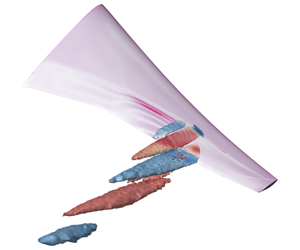
Figure 7. Spatial structure of unstable eigenmode SB showing volumetric iso-surfaces at two values ( $\pm 0.02$) of real part of
  $x$-momentum component
  $\widehat{\unicode[STIX]{x1D70C}u}$ and in (a) real part of surface pressure amplitude
  $\widehat{C}_{p}$ and (b) surface pressure coefficient
  $\bar{C}_{p}$. Base-flow zero-skin-friction line is indicated by a dark grey line. The eigenvector has been scaled by the maximum
  $x$-momentum value, found at approximately
  $(x,y,z)=(1.170,0.546,0.160)$ and indicated by the yellow sphere. Dash-dotted lines in (b) describe the spanwise cuts to be presented in figures 8 and 9.
The spatial structure of the unstable global mode SB at  $\unicode[STIX]{x1D6FC}=3.75^{\circ }$ is presented in figure 7, visualising buffet cells. The term buffet cell refers to a localised three-dimensional cellular pattern with a flow arrangement of a ripple along the spanwise shock wave combined with a pulsating shear layer, which develops within a restricted sector of the wingspan. Coherent spatial amplitudes of the shock-buffet mode are concentrated at the shock wave and its downstream shear layer. In the figures only the real part of the complex-valued eigenvector, scaled by the maximum value of the
  $x$-momentum component, is shown since the corresponding imaginary part is spatially 90° out-of-phase to enable the description of travelling flow structures via reconstruction of the physical signal using equation (2.1) (Crouch et al. Reference Crouch, Garbaruk and Magidov2007; Sipp et al. Reference Sipp, Marquet, Meliga and Barbagallo2010). The propagation path of these buffet-cell structures is chordwise downstream and spanwise outboard, while there is wing support in the sector
  $\unicode[STIX]{x1D702}\approx 0.6$ to 0.73, and then downstream in the wake, going beyond the horizontal-tail plane. It is interesting to observe that the spatial structures of the three-dimensional shock-buffet mode originate at the wing surface near the outermost portion of the reverse-flow region, as enclosed by the base-flow zero-skin-friction line in figure 7(b) just outboard of the Yehudi break. Since the sign of the skin-friction coefficient is based on the streamwise velocity component, this suggests that the buffet cells emerge in the vicinity of where reversed flow is forced to turn back into the main streamwise flow direction. The impact of mesh refinement focussing on the unstable mode is scrutinised in a brief study in appendix A. Closer inspection of the coherent structures, while the corresponding eigenvalue of the critical shock-buffet mode migrates from its
  $\unicode[STIX]{x1D6FC}=3.6^{\circ }$ position, which is when the leading mode can first easily be identified unambiguously from the rest of the spectrum – in figure 6, extrapolation of the same mode to
  $\unicode[STIX]{x1D6FC}=3.5^{\circ }$ gives a damping ratio of
  $\unicode[STIX]{x1D70E}\approx -0.5$, well within the dense cloud rendering it inaccessible with the methods presented – to
  $\unicode[STIX]{x1D6FC}=4.0^{\circ }$ (not shown in the figure), suggests that the appearance of the spatial amplitudes remains similar without marked changes to their topology. Visual inspection of the other eigenmodes with reduced decay rate (cf. figure 6 for Strouhal numbers
  $St\approx 0.3$ to 0.7) follows below in figure 11.

Figure 8. Slices at constant spanwise stations  $\unicode[STIX]{x1D702}=0.603$ (a–c),
  $\unicode[STIX]{x1D702}=0.660$ (d–f) and
  $\unicode[STIX]{x1D702}=0.727$ (g–i) showing real part of eigenvector’s momentum components with
  $x$-momentum
  $\widehat{\unicode[STIX]{x1D70C}u}$ (a,d,g),
  $y$-momentum
  $\widehat{\unicode[STIX]{x1D70C}v}$ (b,e,h) and
  $z$-momentum
  $\widehat{\unicode[STIX]{x1D70C}w}$ (c,f,i). The sonic line is highlighted by a dash-dotted line.

Figure 9. Slice at constant spanwise station  $\unicode[STIX]{x1D702}=0.660$ showing real part of eigenvector’s scalar quantities with density
  $\widehat{\unicode[STIX]{x1D70C}}$ (a), total energy
  $\widehat{\unicode[STIX]{x1D70C}E}$ (b) and turbulence-field variable
  $\widehat{\unicode[STIX]{x1D70C}\tilde{\unicode[STIX]{x1D708}}}$ (c). The sonic line is highlighted by a dash-dotted line.
In figures 8 and 9 the complex-valued amplitude functions of the conservative variables are presented at constant spanwise stations. The momentum components are given at three stations with  $\unicode[STIX]{x1D702}=0.603$, 0.660 and 0.727, as indicated in figure 7(b) by dash-dotted lines, of which the inner and outer locations correspond to those in figure 3. The scalar variables of density and total energy and the turbulence-field variable of the Spalart–Allmaras model are only shown at
  $\unicode[STIX]{x1D702}=0.660$. At individual spanwise stations, a certain similarity with the description of the two-dimensional aerofoil shock-buffet mode is striking. Specifically, the analysis by Sartor et al. (Reference Sartor, Mettot and Sipp2015) shall be mentioned, who, for example, emphasised a synchronisation with opposite signs in the
  $x$-momentum component
  $\widehat{\unicode[STIX]{x1D70C}u}$ within the shock wave and its downstream shear layer. While the shock moves downstream, their bubble contracts, and vice versa. A complicating factor herein is the added spatial three-dimensionality with propagation not only chordwise but also spanwise, which can be noticed in the lag of
  $x$-momentum structures downstream in the wake region (cf. figure 7b). Comparing streamwise and spanwise momentum components, their amplitudes are of similar magnitude, hence highlighting the strong crossflow contribution. Inspecting the turbulence-field variable
  $\widehat{\unicode[STIX]{x1D70C}\tilde{\unicode[STIX]{x1D708}}}$, blobs of high eddy-viscosity fluctuations in the wake can be inferred, albeit significantly reduced magnitude compared with the other conservative amplitude functions. This is typical for unsteady RANS simulations of shock buffet (Sartor & Timme Reference Sartor and Timme2017) and relates to high turbulence levels in the buffet cells which result from the shock-wave/boundary-layer interaction.

Figure 10. Spatial structure of unstable eigenmode SB showing magnitude  $|\widehat{C}_{p}|$ of surface pressure coefficient over entire wing surface and selected outboard spanwise stations. Base-flow pressure coefficient
  $\bar{C}_{p}$ (black line) is included for orientation. Also shown is the base-flow zero-skin-friction line in the surface plot (dark grey line). Experimental data at
  $Re\approx 1.5\times 10^{6}$ for spanwise station
  $\unicode[STIX]{x1D702}=0.603$ were taken from Koike et al. (Reference Koike, Ueno, Nakakita and Hashimoto2016) using the root-mean square pressure fluctuations (plotted at arbitrary scale) at angles of attack
  $\unicode[STIX]{x1D6FC}=3.35^{\circ }$ (○) and 3. 88° (●) to bracket
  $\unicode[STIX]{x1D6FC}=3.75^{\circ }$ discussed herein.
Figure 10 gives an idea of the magnitude of perturbation in the pressure coefficient,  $|\widehat{C}_{p}|$. The surface plot reveals that highest levels of unsteadiness are found outboard of the base-flow reverse-flow region, extending along the shock towards the wing tip and highlighting the centre of strong shear-layer pulsation between shock location and trailing edge. It must be emphasised that the linear eigenmode predicts the prominent shear-layer fluctuations just outboard of where the base flow suggests reverse flow with respect to the
  $x$-velocity component. These regions do not coincide spatially. A similar conclusion can be reached by inspecting the surface skin-friction fluctuation (not shown herein). Information at several spanwise stations offers a fuller picture. Note that the steady-state pressure distribution (cf. figure 3) is included in the plots at each spanwise station to demonstrate more clearly the relation between base-flow shock position and unsteady pressure perturbation. Particulars of the perturbation peaks observed at the shock location are typical for linearised frequency-domain techniques, which is at the heart of our stability tool (Thormann & Widhalm Reference Thormann and Widhalm2013). At station
  $\unicode[STIX]{x1D702}=0.502$, pressure-fluctuation levels are approximately three orders of magnitude lower than the peak values at the other stations, and those fluctuations are of similar magnitude on the upper and lower surface of the wing. The other spanwise stations show significantly higher fluctuations on the upper surface compared with the lower one. In particular, the shock motion and linked shear-layer pulsation dominate the picture. Note, albeit similar levels of pressure fluctuation, the axis scaling for stations
  $\unicode[STIX]{x1D702}=0.603$ and 0.846 differs by a factor of five for two reasons. First, the intention is to accentuate the reduction in shock unsteadiness towards the wing tip between stations
  $\unicode[STIX]{x1D702}=0.660$ and 0.846. Second, for the sake of clarity, experimental data points are included at station
  $\unicode[STIX]{x1D702}=0.603$ which were taken from Koike et al. (Reference Koike, Ueno, Nakakita and Hashimoto2016) based on measurements from unsteady pressure transducers. The root-mean square pressure fluctuations at two angles of attack, bracketing our critical condition, are presented at arbitrary scale. Compare with figure 17 for those experimental data to be shown at consistent scale. Agreement regarding the chordwise location of pressure fluctuation is rather good. Note the lack of experimental unsteady pressure sensors between
  $x/c=0.36$ and 0.50. Koike et al. (Reference Koike, Ueno, Nakakita and Hashimoto2016) presented additional unsteady pressure data at spanwise station
  $\unicode[STIX]{x1D702}=0.50$, where equivalent numerical data herein in figure 10 (and also in figure 17 to follow) show insignificant activity altogether.
It is hence important to re-emphasise that the experimental data for the 80 %-scale model of the same wing geometry stem from a threefold decrease in Reynolds number ( $Re\approx 1.5\times 10^{6}$). Koike et al. (Reference Koike, Ueno, Nakakita and Hashimoto2016) discussed the impact of Reynolds-number variation on the chordwise shock position, and consequently, a minor downstream shift is expected herein. As noted earlier, Dor et al. (Reference Dor, Mignosi, Seraudie and Benoit1989) judged the Reynolds-number influence on the dynamics of shock buffet as negligible, at least for the variance in pressure fluctuations for an aerofoil, provided the shock-wave/boundary-layer interaction is fully turbulent. Besides Reynolds number effecting the flow development, the deformation of a flexible wing under load, both static and dynamic, must be accounted for, too. Different physical wing structures, although featuring nominally the same aerodynamic geometry, were examined under different test conditions (e.g. total pressure in the wind tunnel), presumably without regard to aeroelastic scaling. Careful inspection of the available data in the literature at angles of attack near our focus angle (
 $\unicode[STIX]{x1D6FC}=3.75^{\circ }$) gives a wing-tip bending of 0.023 (per semi-span) and a twist of -1. 2° (wash-out) for the ETW test (Keye & Gammon Reference Keye and Gammon2018) compared with 0.012 and -0. 7° for the JAXA test (Koike et al. Reference Koike, Ueno, Nakakita and Hashimoto2016). Differences in the underlying structural model can also be inferred from the relative wash-in twist near the wing tip on the 80 %-scale model. The present study accounts for static deformation measured in the ETW test campaign. This brief discussion highlights a key message of this work. Numerical analysis of the pure aerodynamics (be it global stability or time-marching methods) can only explain part of the complex interaction relating to shock-induced separation and shock unsteadiness on a flexible wing. Multidisciplinary studies are needed to quantify various factors including, but not limited to, wind tunnel noise and structural dynamics (Steimle et al. Reference Steimle, Karhoff and Schröder2012; Masini et al. Reference Masini, Timme and Peace2020).

Figure 11. Eigenvalue spectra at three angles of attack approaching (and beyond) shock-buffet onset and corresponding spatial structure of representative modes at  $\unicode[STIX]{x1D6FC}=3.75^{\circ }$ showing volumetric iso-surfaces at two values (
 $\pm 0.02$) of real part of
  $x$-momentum component
  $\widehat{\unicode[STIX]{x1D70C}u}$. Eigenvectors have been normalised by the
  $x$-momentum value at
  $(x,y,z)=(1.170,0.546,0.160)$ to set magnitude and phase at this point consistently to one and zero, respectively. Wing-surface colouring describes the real part of pressure amplitude
  $\widehat{C}_{p}$, while solid line is the zero-skin-friction line. Dash-dotted lines, included for the leading shock-buffet mode SB, almost perpendicular to the shock give an indication of how the spanwise wavelength of modes is estimated.
As hinted above, figure 11 shows a portion of the eigenspectrum, where the pure aerodynamic shock-buffet instability is found, at three angles of attack around onset together with the spatial structure of a number of physically dominant eigenmodes at  $\unicode[STIX]{x1D6FC}=3.75^{\circ }$. A correlation between the modes’ frequencies and their spatial structures, represented by volumetric iso-surfaces of the real part of
  $x$-momentum component
  $\widehat{\unicode[STIX]{x1D70C}u}$ at non-dimensional values of
  $\pm 0.02$, is evident. Eigenvectors have been normalised by their respective
  $x$-momentum value at
  $(x,y,z)=(1.170,0.546,0.160)$, which is the location of the maximum value for mode
  $\text{b}$ in the figure (which is mode SB in figure 7(b)), to ensure that the magnitude and phase at this point are consistently set to one and zero, respectively. Note the increasingly fine-grained coherent structures for modes at higher frequencies, also featuring similar levels of unsteadiness on the horizontal-tail plane. The richness in frequencies and spatial structures could contribute to an explanation (yet to be established) of the often-reported broadband-frequency nature of shock buffet on wings, which is in contrast to aerofoil studies (Jacquin et al. Reference Jacquin, Molton, Deck, Maury and Soulevant2009). Besides the five modes with their spatial structures shown in the figure, there is a large number of unphysical modes in this same frequency range, which neither migrate significantly with increasing angle of attack nor emerge from the dense band/cloud of eigenvalues, but do have a strong contribution from similar coherent structures; yet, those modes also feature increasingly incoherent, nondescript contributions between the near- and far-field domain.
It is intriguing to note recent biglobal stability analyses by Crouch et al. (Reference Crouch, Garbaruk and Strelet2019), Plante et al. (Reference Plante, Dandois, Beneddine, Sipp and Laurendeau2019a) and Paladini et al. (Reference Paladini, Beneddine, Dandois, Sipp and Robinet2019a) on infinite-span geometries assessing wing-sweep effects. The term biglobal refers to a stability analysis in three-dimensional space with two inhomogeneous dimensions (see Theofilis Reference Theofilis2011). The third, homogeneous direction  $z$ (the
  $xy$-plane describes the aerofoil therein) is treated as periodic using
  $\text{e}^{\text{i}\unicode[STIX]{x1D6FD}z}$ where
  $\unicode[STIX]{x1D6FD}$ is the spanwise wavenumber. The authors contemplate unstable stationary (monotone) modes providing a spanwise three-dimensional structure to a nominally aerofoil shock-buffet mode for the unswept wing, which turn into travelling (oscillatory) modes when wing sweep is imposed, with the sweep angle primarily defining the overall frequency range of those modes. Notwithstanding the so-called triglobal stability analysis on a finite-span and swept wing conducted herein, which cautions juxtaposition, the consensus in salient and subtle shock-buffet features is interesting indeed.

Figure 12. Angular frequency (and Strouhal number) as a function of spanwise wavenumber  $\unicode[STIX]{x1D6FD}$ for characteristic medium-frequency band of eigenmodes. Results are made dimensionless using either mean aerodynamic chord (MAC) and free-stream speed
  $U_{\infty }$ or, when defining a plane approximately normal to the quarter-chord line, local chord
  $c_{n}$ at the location of coherent cellular structures and velocity
  $U_{\infty ,n}$. Labelling of individual modes follows figure 11.
More specifically, figure 12 presents an attempt to characterise the band of eigenvalues emerging from the dense cloud for angles of attack approaching the onset. The figure shows angular frequency  $\unicode[STIX]{x1D714}$ over spanwise wavenumber
  $\unicode[STIX]{x1D6FD}$. Note that the estimation of
  $\unicode[STIX]{x1D6FD}$ is rather rough since it is very difficult to discern fully developed periodicity along the span for a finite wing with localised cellular pattern (which is in contrast to the infinite-wing stability results in Crouch et al. (Reference Crouch, Garbaruk and Strelet2019), Plante et al. (Reference Plante, Dandois, Beneddine, Sipp and Laurendeau2019a) and Paladini et al. (Reference Paladini, Beneddine, Dandois, Sipp and Robinet2019a)). The subplot in figure 11 for mode SB includes dash-dotted lines nearly perpendicular to the shock giving an indication of how the wavelength (
 $l=2\unicode[STIX]{x03C0}/\unicode[STIX]{x1D6FD}$) of modes is estimated based on the coherent structures. Consequently, using the classical definition of the phase velocity, the buffet cells propagate with the speed
  $U_{c}=\unicode[STIX]{x1D714}/\unicode[STIX]{x1D6FD}$. Based on the analysis with non-dimensionalisation using free-stream speed
  $U_{\infty }$ and MAC, the phase speed is in the range 0.26 to 0.32, whereby a gradual increase is observed with decreasing wavelength. The figure includes equivalent results using instead for non-dimensionalisation the reference values in a plane normal to the quarter-chord line with
  $\unicode[STIX]{x1D6EC}_{c/4}=35^{\circ }$, specifically
  $U_{\infty ,n}=U_{\infty }\cos (\unicode[STIX]{x1D6EC}_{c/4})$ and local chord length
  $c_{n}=c\,\cos (\unicode[STIX]{x1D6EC}_{c/4})$ at the location of coherent structures, where
  $c$ is approximately
  $2/3\,\text{MAC}$. It is interesting to note (whether coincidental or not) that the leading unstable mode SB has a wavelength
  $l\approx c$. Besides the difficulty in establishing the length and position of a developed spatial periodicity, also the choice of an appropriate sweep angle is equivocal since the wing is tapered (i.e. leading-edge, quarter-chord and trailing-edge lines differ in their respective sweep angles, so does the shock front). Based on the alternative reference velocity and length scale, the speed of propagation takes values between 0.30 and 0.37. Finally, the figure includes both an empirical model linking the sweep angle to the phase speed (Paladini et al. Reference Paladini, Beneddine, Dandois, Sipp and Robinet2019a) – in our non-dimensional notation
  $\unicode[STIX]{x1D714}=0.76\,\tan (\unicode[STIX]{x1D6EC})\,\unicode[STIX]{x1D6FD}$ with sweep angle
  $\unicode[STIX]{x1D6EC}=30^{\circ }$ – and results taken from Crouch et al. (Reference Crouch, Garbaruk and Strelet2019) at the same sweep angle. Those reference data are for spanwise-infinite wings using the OAT15A aerofoil. The data taken from Crouch et al. (Reference Crouch, Garbaruk and Strelet2019) have been rescaled with respect to the reference velocity normal to the leading edge to be consistent with the definition used in Paladini et al. (Reference Paladini, Beneddine, Dandois, Sipp and Robinet2019a). It appears that our relevant triglobal modes discretise the continuous medium-wavelength band of modes, first presented by Crouch et al. (Reference Crouch, Garbaruk and Strelet2019), albeit necessary secondary geometric features of the finite wing (such as taper and twist), suspected to modify the development of those modes (Plante et al. Reference Plante, Dandois and Laurendeau2019b). Nonetheless, triglobal stability analysis of such infinite wings benefits clearer interpretation of biglobal studies and their relation to a finite wing with complex geometry (He & Timme Reference He and Timme2020).
Those additional eigenvalues with reduced decay rate also show a similar pattern as presented by Timme & Thormann (Reference Timme and Thormann2016) for the pre-onset condition on an older-generation wing design, hence hinting at a universal wing buffet mechanism, and could play a role in explaining the often-reported (and widely accepted) broadband-frequency nature of wing shock buffet beyond onset conditions. Analysis of corresponding conventional time-marching simulation of the saturated nonlinear state at angle of attack  $\unicode[STIX]{x1D6FC}=3.75^{\circ }$, to be discussed in figure 14, will reveal that close to instability onset the broadband nature is not well established. First recall that the analysis herein targets the onset of the alleged Hopf oscillator called shock buffet and not fully developed shock-buffet conditions well beyond onset angle of attack. A second contributing point in this discussion concerns the inherent nonlinearity of the dynamics of shock-wave/boundary-layer interaction, which is elucidated later with the help of figures 14 through 17. Third, when thoroughly comparing with experimental data, the flexible wing structure exposed to a noisy testing environment must not be ignored at these extreme flow conditions, which makes the aerodynamics-only shock-buffet instability and the structural buffeting response a multidisciplinary challenge indeed. The current results shed light on a pure aerodynamic instability but at the same time cannot explain everything that is going on in the wind tunnel. For instance, Masini et al. (Reference Masini, Timme, Ciarella and Peace2017, Reference Masini, Timme and Peace2020) reported distinct lower-frequency shock dynamics, even before the onset of a structural buffeting response in the root strain-gauge signal, with an inboard propagation direction and widely extending along the span. The frequency content is stated to be in the range of aerofoil shock-buffet frequencies, whether this is coincidental or not. Similar behaviour was briefly mentioned by Dandois (Reference Dandois2016). Numerically, small-amplitude forced wing vibration also revealed resonant aerodynamic response for
  $St\approx 0.1$, besides the accepted shock-buffet range with
  $St\approx 0.3$ to 0.7 (Timme & Thormann Reference Timme and Thormann2016; Belesiotis–Kataras & Timme Reference Belesiotis–Kataras and Timme2018). In any case, our computations paid special attention to these lower frequencies trying to identify another absolute instability mechanism, without success. Nevertheless, these findings in the transonic flow over a wing do not rule out an additional instability of convective nature (i.e. a noise amplifier) and pseudo-resonance due to the non-normality of the governing equations (Trefethen et al. Reference Trefethen, Trefethen, Reddy and Driscoll1993; Sipp et al. Reference Sipp, Marquet, Meliga and Barbagallo2010; Sartor et al. Reference Sartor, Mettot and Sipp2015). Finally, eddy-resolving simulation is required to better account for the influence of strong turbulent fluctuations resulting from the shock-wave/boundary-layer interaction. Having said this, while Sartor & Timme (Reference Sartor and Timme2017) observed a broadband nature due to irregular shock dynamics and patterns of flow separation using delayed detached-eddy simulation as well as unsteady RANS modelling well beyond shock-buffet onset, Masini, Timme & Peace (Reference Masini, Timme and Peace2019) demonstrated far less pronounced broadbandedness in the shock-buffet dynamics using similar scale-resolving simulation in close vicinity to the onset on a rigid wing.
The argument is made that our results qualitatively and quantitatively reproduce findings documented in existing literature reporting on wing shock-buffet features. Inspecting the data-based modes from dynamic mode decomposition (in contrast to our operator-based modes (Taira et al. Reference Taira, Brunton, Dawson, Rowley, Colonius, McKeon, Schmidt, Gordeyev, Theofilis and Ukeiley2017)) identified from a detached-eddy simulation on the 80 %-scale model of the same wing in well-established shock-buffet condition (Ohmichi et al. Reference Ohmichi, Ishida and Hashimoto2018), frequencies, spatial structures and their locations agree nicely overall, despite a discarded fuselage geometry therein. The latter numerical study itself followed the experimental campaign, mentioned earlier, at reduced Reynolds number documented in Koike et al. (Reference Koike, Ueno, Nakakita and Hashimoto2016) and Sugioka et al. (Reference Sugioka, Koike, Nakakita, Numata, Nonomura and Asai2018). On an older 1970s wing, experimental and numerical work revealed the shock-buffet cells, albeit positioned further outboard towards the wing tip (Lawson et al. Reference Lawson, Greenwell and Quinn2016; Sartor & Timme Reference Sartor and Timme2017; Masini, Timme & Peace Reference Masini, Timme and Peace2018; Masini et al. Reference Masini, Timme and Peace2019, Reference Masini, Timme and Peace2020). Other notable work includes the analysis of wind tunnel data on different transport-type wings (Dandois Reference Dandois2016; Paladini et al. Reference Paladini, Dandois, Sipp and Robinet2019b) and the hierarchical study of canonical geometric complexity (such as wing sweep) and its impact on shock-buffet characteristics using time-marching unsteady RANS (Iovnovich & Raveh Reference Iovnovich and Raveh2015; Plante et al. Reference Plante, Dandois and Laurendeau2019b) and biglobal stability theory (Crouch et al. Reference Crouch, Garbaruk and Strelet2019; Plante et al. Reference Plante, Dandois, Beneddine, Sipp and Laurendeau2019a; Paladini et al. Reference Paladini, Beneddine, Dandois, Sipp and Robinet2019a). Reflecting on such biglobal work, salient and subtle features of the instability seem consistent. More specifically, He & Timme (Reference He and Timme2020) demonstrate for the infinite wing how triglobal analysis, which is fully equivalent to the methods used herein, reproduces the continuous band of spanwise modes in the medium-wavelength range discretely (cf. figure 12). Crouch et al. (Reference Crouch, Garbaruk and Strelet2019) contemplate the broadbandedness on swept wings to result from an (as yet unquantified) interaction of modes.
4.2 Symmetry and anti-symmetry

Figure 13. Eigenvalue spectra for half- and full-span computations and corresponding spatial structure of representative full-span modes showing iso-surfaces at two values ( $\pm 0.02$) of real part of
  $x$-momentum component
  $\widehat{\unicode[STIX]{x1D70C}u}$. Eigenvectors have been scaled by the
  $x$-momentum at
  $(x,y,z)=(1.170,0.546,0.160)$ to set magnitude and phase at this point consistently to one and zero, respectively. Wing-surface colouring describes real part of pressure amplitude
  $\widehat{C}_{p}$, while solid line is zero-skin-friction line. Subscripts
  $\text{S}$ and
  $\text{A}$ indicate symmetric and anti-symmetric modes, respectively. Symmetric modes correspond to half-model results in figure 11.

Figure 14. Time histories of integrated coefficients around base-flow solution showing (a) initial linear regime of lift coefficient from time-marching unsteady RANS simulations, bracketing buffet onset between  $\unicode[STIX]{x1D6FC}=3.50^{\circ }$ and 3. 75°, and comparison with signal reconstructed from unstable eigenmode at
  $\unicode[STIX]{x1D6FC}=3.75^{\circ }$, and (b) and (c) the effect of nonlinear saturation on coefficients of lift and drag, respectively. Chosen instantaneous time steps to be presented in figures 15 and 16 are indicated by Roman numerals in (d) for the final cycles of the linear regime, just before nonlinear effects become dominant, and (e) and (f) for the saturated nonlinear regime.
The discussion continues with a study of the impact of (not) enforcing symmetry boundary condition at the fuselage centre plane. Figure 13 shows the relevant part of the eigenspectra for the half- and full-span models at angle of attack  $\unicode[STIX]{x1D6FC}=3.75^{\circ }$. Labelling of eigenmodes follows figure 11. We observe pairs of eigenvalues (not referring to the complex conjugate pairs, which exist, too), labelled with subscripts
  $\text{S}$ and
  $\text{A}$ for symmetric and anti-symmetric, respectively. At first glance, the unstable eigenvalue (labelled
  $\text{b}$) seems to have approximately algebraic multiplicity of 2. For the remaining dominant eigenvalues, one of each pair coincides with the half-span result, while the second one is slightly shifted. This behaviour was scrutinised in more detail. Appreciating that we use iterative solution methods with an approximate linear solver, convergence criteria imposed on base flow (10-13) as well as inner (10-9) and outer (10-8) Krylov methods were further reduced by two orders of magnitude compared with parameter settings in table 1. The results suggest that also the eigenvalues with positive growth rate are distinct. Similar modal characteristics were observed by He et al. (Reference He, Tendero, Paredes and Theofilis2017) for an elliptic wing at low Reynolds number. Note that these pairs of eigenmodes were calculated independent of the chosen shift
  $\unicode[STIX]{x1D701}$. Most importantly, the corresponding pairs of eigenvectors show symmetric and anti-symmetric behaviour. Specifically, for the symmetric case, coherent structures of all conservative variables are mirrored with respect to the fuselage centre plane, such as
  $\widehat{\unicode[STIX]{x1D70C}u}_{port}=\widehat{\unicode[STIX]{x1D70C}u}_{starboard}$, except the
  $y$-momentum component with
  $\widehat{\unicode[STIX]{x1D70C}v}_{port}=-\widehat{\unicode[STIX]{x1D70C}v}_{starboard}$, and vice versa for the anti-symmetric modes. Agreement of the symmetric full-span modes with the half-span results is expected since symmetry boundary condition is consistently enforced in the half-span simulation set-up. The occurrence of anti-symmetric modes means that the dynamic manifestation of the shock-buffet instability on starboard and port sides of the aircraft does not have to be synchronised. Hence, the dynamical system permits realistic non-symmetric perturbations, as should be expected in general.
4.3 Time-marching analysis
To further support the findings, integrated and distributed time-marching unsteady RANS results are consulted. Integrated aerodynamic coefficients of lift and drag, specifically the perturbations around the base-flow solution, exemplified in the following for the lift coefficient as  $\widetilde{C}_{L}=C_{L}-\bar{C}_{L}$, are shown in figure 14(a–c) as a function of non-dimensional time
  $t$. Figure 14(d–f) gives the corresponding total values of the same coefficients during one fundamental oscillation cycle together with an indication of the time steps where distributed surface pressures will be presented in figures 15 and 16 for the linear and nonlinear regime, respectively. Conventional time-marching results at angle of attack
  $\unicode[STIX]{x1D6FC}=3.75^{\circ }$ are also compared with the unsteady aerodynamic coefficient calculated from the unstable global mode using, e.g. for the lift coefficient, the relation
  $\widetilde{C}_{L}(t)=\widehat{C}_{L}\,\text{e}^{\unicode[STIX]{x1D706}t}+\text{c.c}$. The latter equation ensures that a real-valued physical signal is reconstructed from the complex-valued eigenmode, with the eigenvector prescribing magnitude and phase of a damped harmonic oscillator in each mesh point and flow variable, and with oscillation frequency (and exponential envelope function) provided by the eigenvalue. Conveniently, the complex-valued amplitude of e.g. the lift coefficient, denoted
  $\widehat{C}_{L}$, is calculated directly from the eigenvector using the expression
  $\widehat{C}_{L}=\unicode[STIX]{x2202}C_{L}/\unicode[STIX]{x2202}\boldsymbol{u}\boldsymbol{\cdot }\widehat{\boldsymbol{u}}$, which is widely known in the context of (dynamic) derivative and adjoint gradient computations. In essence, the latter equation provides the integration of the conservative variables over solid walls. The partial derivative
  $\unicode[STIX]{x2202}C_{L}/\unicode[STIX]{x2202}\boldsymbol{u}$, computed once for the base flow to describe the lift dependence on the conservative variables, is a functionality readily available in the chosen flow solver and generalises to any integrated aerodynamic load. This means that post-processing is very effective without the need otherwise to feed the computed unsteady field solution of the conservative variables, which can also be reconstructed from the eigenmode (cf. equation (2.1)), back into the nonlinear flow solver. Since the eigenvector
  $\widehat{\boldsymbol{u}}$ can be scaled arbitrarily, and the time-marched solution is integrated in time from an initial condition of white noise, its magnitude is adjusted manually to align with the time-domain results.

Figure 15. Time evolution of unstable eigenmode showing disturbance in surface pressure coefficient,  $\widetilde{C}_{p}=C_{p}-\bar{C}_{p}$, at six time steps during one oscillation cycle; cf. figure 14(d). Instantaneous reverse-flow regions are indicated by the dark grey zero-skin-friction lines.

Figure 16. Time evolution of surface pressure coefficient,  $C_{p}$, at six time steps during one fundamental, nonlinearly saturated oscillation cycle; cf. figure 14(e,f). Instantaneous reverse-flow regions are indicated by the dark grey zero-skin-friction lines.
In figure 14(a), time histories of the lift coefficient locate the onset of shock-buffet instability between angles of attack  $\unicode[STIX]{x1D6FC}=3.50^{\circ }$ and 3. 75°. No attempt is made to refine this bracket further using time-marching simulations. Agreement between the conventional time-marching simulation and global stability analysis is excellent in the linear-amplitude regime up to approximately non-dimensional time
  $t=95$. When growing from white-noise disturbances due to imperfectly converged base flow, the initial linear dynamics is dominated by the leading eigenmode. Since the underlying physics of wing shock buffet is highly nonlinear, nonlinear saturation leading to limit-cycle oscillation is expected. This behaviour is made clearer in figure 14(b,c) for coefficients of lift and drag, respectively. With a base-flow lift coefficient of
  $\bar{C}_{L}=0.6058$, the amplitude nonlinearity takes over when the unsteady lift perturbation reaches approximately 0.15 % of its base-flow value. The terminal limit-cycle amplitude reaches about 0.45 % of the base-flow value with its time-averaged mean dropping approximately 1.5 % below the base-flow lift coefficient. Recall that stability analysis of the steady base flow, which is a solution of the discretised nonlinear RANS equations (plus turbulence model), is performed herein. In contrast, the time-averaged mean flow is not such an equilibrium solution. Subtleties of this distinction have been discussed in the past (e.g. in Barkley (Reference Barkley2006), Sipp & Lebedev (Reference Sipp and Lebedev2007) and Mettot et al. (Reference Mettot, Sipp and Bézard2014)). With a base-flow drag coefficient of
  $\bar{C}_{D}=0.04196$, similar values are found for the drag coefficient albeit the time-averaged mean increasing by seven drag counts, highlighting the inevitable drag penalty. The low limit-cycle amplitude at angle of attack
  $\unicode[STIX]{x1D6FC}=3.75^{\circ }$ confirms the vicinity to the instability onset (and possibly the existence of a supercritical Hopf bifurcation). Also observe the rather regular oscillations in the nonlinear regime, albeit clear higher harmonic contributions, as seen in figure 14(e) and (f) for one oscillation cycle, compared with the single-harmonic exponential growth in figure 14(d). The presented time window of three non-dimensional time units in figure 14(d–f) was deliberately chosen trying to highlight the increase in oscillation frequency in the nonlinear regime. Fourier analysis of the linear stage shows a peak at about
  $\unicode[STIX]{x1D714}=2.36$ (
 $St=0.376$), obviously corresponding to the rightmost eigenvalue, whereas this shifts to
  $\unicode[STIX]{x1D714}=2.62$ (
 $St=0.417$) during the nonlinear response.
Figures 15 and 16 show the time evolution of the surface pressure coefficient in the outer wing region at six time steps during one fundamental period of oscillation, as indicated in figure 14(d–f). For the sake of clarity, since pressure fluctuations in the linear regime are too insignificant to deform the shock discernibly, figure 15 visualises only the linear perturbation in pressure coefficient around the base flow,  $\widetilde{C}_{p}=C_{p}-\bar{C}_{p}$. As explained just above for the unsteady lift coefficient, for the flow-field reconstruction from the leading (unstable) eigenmode, the expression
  $\widetilde{C}_{p}(\boldsymbol{x},t)=\widehat{C}_{p}(\boldsymbol{x})\,\text{e}^{\unicode[STIX]{x1D706}t}+\text{c.c.}$ is used. For the linear regime, the discussion can mostly follow the description of the spatial structure of the unstable eigenmode in figure 10. We can see pressure perturbations travelling along the shock towards the wing tip together with the pressure footprint of the pulsating shear layer between
  $\unicode[STIX]{x1D702}=0.660$ and 0.727 outboard of the instantaneous reverse-flow region, which itself closely resembles the base flow. This suggests that the flow unsteadiness is not substantial enough to break up the enclosed separation pattern, which is in contrast to the nonlinear regime discussed in figure 16. The repeated spanwise outboard (and chordwise downstream) propagation of localised buffet cells is indeed corroborated. The phase speed
  $U_{c}$ of those cellular patterns along the span just downstream of the shock position is cautiously estimated from this spatial structure and is found to be about
  $U_{c}\approx 0.28$ (normalised by free-stream speed
  $U_{\infty }$), which agrees nicely with figure 12.

Figure 17. Standard deviation of surface pressure coefficient,  $C_{p,stdev}$, in the nonlinear regime, computed in a duration of approximately 30 non-dimensional time units, over the entire wing surface and selected outboard spanwise stations. Pressure coefficients of base flow (solid black line) and mean flow (dashed dark grey line) are included for orientation. Also shown is mean-flow reverse-flow region in the surface plot (dark grey line). Experimental root-mean square data of pressure fluctuations for spanwise station
  $\unicode[STIX]{x1D702}=0.603$ at angles of attack
  $\unicode[STIX]{x1D6FC}=3.35^{\circ }$ (○) and 3. 88° (●) were taken from Koike et al. (Reference Koike, Ueno, Nakakita and Hashimoto2016) (at
  $Re\approx 1.5\times 10^{6}$) to bracket
  $\unicode[STIX]{x1D6FC}=3.75^{\circ }$ discussed herein.
Figure 16, on the other hand, presents the total values in the nonlinear regime to emphasise the spanwise shock oscillation and highly irregular localised reverse-flow patterns. Comparing with figure 15, there are clear signs that the unsteadiness is sustained through the linear instability. For instance, the innermost position of shock deformation around  $\unicode[STIX]{x1D702}=0.603$ agrees with the spatial amplitudes of the eigenmode, the shock deformation itself emerges from the nonlinear amplification of the instability, and its direction of travel remains outboard. In contrast, the shock disturbance is substantial enough to break up the outermost portion of the otherwise enclosed reverse-flow region irregularly. Also, those strong shock disturbances travelling outboard result in localised pockets of separation up to
  $\unicode[STIX]{x1D702}=0.846$, with the average chordwise shock position moving upstream, which is reflected in the reduced time-averaged lift coefficient seen in figure 14(b).
The last observation is made clearer in figure 17 showing the standard deviation of the surface pressure coefficient, similar to the magnitude plot in figure 10. The graphs focussing on different spanwise stations additionally include both the base-flow and mean-flow pressure distributions. The surface plot of the standard deviation resembles in parts the results from the eigenvector, and effectively follows what has been discussed in figure 16. The region of shock unsteadiness is more widespread, both chordwise and spanwise. A distinct region can be observed between  $\unicode[STIX]{x1D702}=0.727$ and 0.846, which is the location where the prominent ripple of shock deformation disappears (see for instance time step V in figure 16). Downstream of this region, highest values in shear-layer activity can be observed, even though increased unsteadiness in the shear layer, compared with the linear dynamics, can be identified over a wider spanwise extent. Note that, despite finding localised pockets of flow separation instantaneously, the time average remains enclosed, albeit a reduced spanwise extent compared with the base flow. Looking into detail, the activity on the upper surface at spanwise station
  $\unicode[STIX]{x1D702}=0.502$ compared with the lower one is higher, which is in contrast to the eigenmode at this station (cf. figure 10). Also, while station
  $\unicode[STIX]{x1D702}=0.660$ in figure 10 was most pronounced in terms of shock unsteadiness, the remaining stations in figure 17 all show a similar level of pressure fluctuations. The chordwise extent of activity is increased due to the more substantial shock deformation, which also reaches closer to the wing tip. Finally, a smearing of the mean-flow shock compared with the crisp base-flow discontinuity can be reported. The spanwise station
  $\unicode[STIX]{x1D702}=0.603$ also includes experimental results taken from Koike et al. (Reference Koike, Ueno, Nakakita and Hashimoto2016). Surprisingly good agreement is observed, despite a lack of pressure sensors between about
  $x/c=0.36$ and 0.50 and the differences pointed out earlier when discussing figure 10. Unfortunately, experimental time-resolved and spectral data analysis closer to the onset angle of attack for the 80 %-scale model has not been published (Sugioka et al. Reference Sugioka, Koike, Nakakita, Numata, Nonomura and Asai2018).
5 Conclusions
Eigenmodes of a practical test case with three inhomogeneous spatial dimensions, specifically an aircraft wing in high-Reynolds-number, turbulent and transonic flow, have been computed. A matrix-forming iterative scheme of an inner–outer Krylov structure, implemented in an industrial Reynolds-averaged Navier–Stokes flow solver, succeeds in identifying an absolute instability linked to shock-buffet onset on a finite and swept wing for the first time. Albeit using computational aerodynamics with turbulence modelling for the Reynolds stresses, these fundamental results suggest that the incipient departure of shock-buffet unsteadiness from a nonlinear steady base flow is governed by the dynamics of a single unstable oscillatory eigenmode, which eventually is superseded by effects of nonlinear saturation. Increasing the angle of attack beyond onset condition, additional modes from a group of modes, exhibiting reduced decay rate in the vicinity of instability onset and lying within the broadband-frequency range typical reported for large transport-type wings, become unstable. Those physically relevant modes belong to a characteristic medium-wavelength mode form with spanwise wavelengths approximately equal to the local chord, previously identified for infinite wings. Contrary to previous numerical work on infinite straight and swept, untapered configurations, an absolute instability of an aerofoil-like, almost two-dimensional, long-wavelength mode is not established herein, and in this matter the role of the complex wing geometry needs further scrutiny. For the modern wing design of the NASA Common Research Model discussed in this work, the investigated flow condition is a Mach number of 0.85 with reference-chord Reynolds number of  $5.0\times 10^{6}$. Onset occurs just above angle of attack 3. 70° with a Strouhal number of approximately 0.39. The spatial structure of the unstable mode itself, generalising the concept of an aerofoil buffet mode to finite wings, to describe the shock-buffet dynamics, confirms what has been coined shock-buffet cells and inferred previously from numerical and experimental studies on wings.
The numerical findings are surprising in light of the often-used broadband-frequency explanation of three-dimensional shock buffet and have far-reaching implications, going beyond a mere better understanding of edge-of-the-envelope flow physics. This study will inform routes to buffet control via eigenvalue sensitivity and when attempting to establish rapid shock-buffet prediction tools for routine industrial unsteady aerodynamic analysis, such as reduced-order models based on a modal-decomposition-and-projection philosophy. The successful adaptation of an industrial flow solver paves the way to exploit concepts, established in fundamental fluid mechanics research on mostly canonical test cases, in an applied and practical setting. It is anticipated that higher-fidelity eddy-resolving simulations on the rigid wing, to overcome well-known inherent issues of turbulence modelling, will reveal similar low-frequency buffet modes albeit a variety of associated feature-rich phenomena. With an absolute instability confirmed, the role of convective mechanisms in shock-buffet flow physics on wings remains to be scrutinised. In the long-term, fully coupled fluid–structure analysis is desirable when considering the innate multidisciplinary nature of such edge-of-the-envelope flight physics.
Acknowledgements
Part of this work has received funding from the UK Engineering and Physical Sciences Research Council under grant EP/R037027/1. The author is grateful to colleagues at Aircraft Research Association Ltd. (A. Peace) for generating and sharing the meshes and German Aerospace Center (S. Keye) for providing and discussing the wind tunnel data. The author also wishes to thank J. D. Crouch (The Boeing Company) for pointing out the relevance of data analysis leading to figure 12.
Declaration of interests
The author reports no conflict of interest.
Appendix A. Mesh convergence

Figure 18. Mesh refinement for rightmost eigenmode showing (a) volumetric iso-surfaces at two values ( $\pm 0.02$) of the
  $x$-momentum component
  $\widehat{\unicode[STIX]{x1D70C}u}$ for coarsest and finest mesh (see figure 7(b) for medium mesh) and (b) real part of
  $x$-momentum at constant spanwise station
  $\unicode[STIX]{x1D702}=0.660$. Eigenvectors have been scaled by their respective maximum value in
  $x$-momentum, indicated by the yellow spheres, to compare results on different meshes.
In figure 18 (together with figure 7(b) for the top view on the medium mesh) a mesh convergence study is offered to build confidence in the shock-buffet physics presented herein. The slices in the right column, showing the  $x$-momentum component
  $\widehat{\unicode[STIX]{x1D70C}u}$, are taken at constant
  $\unicode[STIX]{x1D702}=0.660$, which locates them approximately at the centre of the three-dimensional spatial structure. Gradually converging results with respect to the mesh density is confirmed; for instance, the features of the spatial structure become more refined with increasing mesh size. Concerning the corresponding eigenvalues (cf. table 2), it is the rightmost eigenvalue in the shock-buffet frequency range, identified in either case. Whereas the growth rate on the coarsest mesh with
  $3.1\times 10^{6}$ points still indicates stable conditions, the two finer meshes predict the instability. Despite a remaining sensitivity in growth rate, the frequencies agree nicely throughout, offering sufficient convergence, as also demonstrated by a relative error of less than 2 % between medium and fine mesh.
Appendix B. Properties of inner–outer Krylov method
Table 2. Mesh convergence of rightmost shock-buffet eigenvalue. Relative error is calculated as  $|1-\unicode[STIX]{x1D706}/\unicode[STIX]{x1D706}_{6.2M}|$ where
  $\unicode[STIX]{x1D706}_{6.2M}$ refers to the eigenvalue on the medium mesh (
 $6.2\times 10^{6}$ points).


Figure 19. Sanity checks on convergence and coverage of eigenmode computations showing (a) norm of Rayleigh quotient error  $|\unicode[STIX]{x1D706}-\widehat{\boldsymbol{u}}^{H}\unicode[STIX]{x1D645}\,\widehat{\boldsymbol{u}}|$ vs. residual norm of eigenvalue problem
  $\Vert \unicode[STIX]{x1D645}\,\widehat{\boldsymbol{u}}-\unicode[STIX]{x1D706}\widehat{\boldsymbol{u}}\Vert$ for all computations at
  $\unicode[STIX]{x1D6FC}=3.50^{\circ }$ and 3. 75° and (b) intersection and union of solutions based on individual shifts at
  $\unicode[STIX]{x1D6FC}=3.75^{\circ }$. Red dots in (a) are the multiple solutions of the unstable mode at 3. 75°. Black dots in (b) are shift locations.
Table 3. Convergence of leading (unstable) eigenmode depending on tolerances of inner and outer iterations using a shift of  $\unicode[STIX]{x1D701}=2.5i$. Size of Krylov space for outer iterations is 25 throughout. Eigenvalues
  $(\unicode[STIX]{x1D70E},\unicode[STIX]{x1D714})$ are truncated at seven significant digits, and residual norm
  $\Vert \unicode[STIX]{x1D645}\,\widehat{\boldsymbol{u}}-\unicode[STIX]{x1D706}\widehat{\boldsymbol{u}}\Vert$ is rounded to closest order of magnitude.

Figure 19 and table 3 aim to establish numerical credibility of presented eigenmode data. In figure 19(a), the norm of the Rayleigh quotient error,  $|\unicode[STIX]{x1D706}-\widehat{\boldsymbol{u}}^{\,H}\unicode[STIX]{x1D645}\,\widehat{\boldsymbol{u}}|$, and the residual norm of the eigenvalue problem,
  $\Vert \unicode[STIX]{x1D645}\,\widehat{\boldsymbol{u}}-\unicode[STIX]{x1D706}\widehat{\boldsymbol{u}}\Vert$, are shown for all computations at angles of attack
  $\unicode[STIX]{x1D6FC}=3.50^{\circ }$ and 3. 75° (being the focus of this study). The default unit-length eigenvector with
  $\Vert \widehat{\boldsymbol{u}}\Vert =1$ is used. These two complementary error measures have previously been reported in Burroughs et al. (Reference Burroughs, Romero, Lehoucq and Salinger2001). The data back the parameter choices made for a robust solution strategy. In the figure, the residual norm does not agree with the convergence criterion set on the outer iteration (cf. table 1), which is due to ARPACK’s approach of assessing convergence based on the Hessenberg matrix, which itself results from the preconditioned shift-and-invert system (Lehoucq et al. Reference Lehoucq, Sorensen and Yang1998). The isolated group in the lower left corner was identified from solving an adjoint problem corresponding to equation (2.3), specifically
  $\unicode[STIX]{x1D645}^{\dagger }\widehat{\boldsymbol{v}}=\unicode[STIX]{x1D706}^{\ast }\widehat{\boldsymbol{v}}$ with
  $\unicode[STIX]{x1D645}^{\dagger }$ as adjoint matrix,
  $\widehat{\boldsymbol{v}}$ as the left/adjoint eigenvector and
  $\unicode[STIX]{x1D706}^{\ast }=\unicode[STIX]{x1D70E}-\text{i}\unicode[STIX]{x1D714}$ as complex conjugate eigenvalue, keeping all other parameters the same. Such favourable convergence should be exploited in future studies. Multiple converged solutions for the same unstable mode at
  $\unicode[STIX]{x1D6FC}=3.75^{\circ }$ due to overlapping search regions are highlighted by red dots in figure 19(a). In figure 19(b), coverage of the relevant part of the eigenspectrum (based on engineering judgement) is sufficient and has a large overlap. The radius of a circle describes the greatest distance between a shift (black dots in the figure) and any of its converged eigenvalues. While such an approach in finding rightmost eigenvalues appears naive, mathematically rigorous algorithms to compute those eigenvalues directly (see for example Elman et al. (Reference Elman, Meerbergen, Spence and Wu2012) and Timme et al. (Reference Timme, Badcock, Wu and Spence2012)) do not seem feasible for the problem size, as yet. In the search for an absolute instability at lower frequencies (see the discussion in § 4.1), numerous additional eigenmode computations with different shifts did not converge to such sought mode. Note that such a globally unstable mode would be isolated from the dense cloud assisting the shift-and-invert Arnoldi method in detecting it more easily. This further supports the notion of a non-existing absolute instability in the frequency range
  $St\lessapprox 0.1$.
Table 3 summarises a succinct investigation of the convergence properties of the iterative solution method. A number of 25 Krylov vectors is used throughout for the outer iterations. Different tolerances are imposed on inner and outer loops, and the convergence of the leading unstable eigenmode, based on a chosen shift  $\unicode[STIX]{x1D701}=2.5i$, is monitored. The table shows both the eigenvalue
  $\unicode[STIX]{x1D706}$ itself and the Euclidean norm of the residual,
  $\Vert \unicode[STIX]{x1D645}\,\widehat{\boldsymbol{u}}-\unicode[STIX]{x1D706}\widehat{\boldsymbol{u}}\Vert$. Two observations can be stated immediately. First, for the chosen numerical scenario, the variation of outer convergence tolerance is ineffective. This can be explained by the target mode’s isolation from other modes. Second, convergence, demonstrated both through the number of significant digits of the eigenvalue and the residual norm, is proportional to the inner tolerance. These tests reaffirm the chosen default settings, as presented in table 1. During these computations also a second mode, specifically the least stable mode in figure 6, denoted mode
  $c$ in figure 11, with eigenvalue
  $(\unicode[STIX]{x1D70E},\unicode[STIX]{x1D714})=(-0.132,2.728)$, got identified but is not included in the table. The conclusions concerning convergence properties remain the same.
Additionally, the size of the outer Krylov space, using values between 10 and 100, was scrutinised (results of which are not shown herein explicitly either). Even the smallest Krylov space allows the computation of the unstable mode at similar convergence levels, which makes the presented stability method very competitive compared with time-marching unsteady RANS to gain rapid engineering insight into the phenomenon during wing design. If more modes are desired, the Krylov space must be increased accordingly.


 Open access