The Dawn of Geostationary Air Quality Monitoring: Case Studies From Seoul and Los Angeles

Introduction

The atmospheric chemistry community has long held a vision for an integrated observing system that provides continuous long-term information at the spatial and temporal resolutions adequate for monitoring air quality at local, regional, and global scales. This vision was first coherently expressed in the Integrated Global Observing Strategy (IGOS) Atmospheric Chemistry Theme Report over a decade ago (IGACO, 2004). While this vision is broadly similar to what has been accomplished in the global meteorological community, its implementation for atmospheric composition is still in its infancy. Satellite observations are an essential component, providing continuous coverage over large areas globally. Observation requirements relevant to air quality from satellites include temporal sampling at ~1-h frequency and horizontal resolution on the order of 10 km (IGACO, 2004; Fishman et al., 2012). These temporal and spatial requirements can be met globally by using a constellation approach that combines multiple geostationary Earth orbit (GEO) platforms, which provide frequent observations over portions of the globe, with low Earth orbit (LEO) platforms, which provide global once-daily coverage (CEOS, 2011). Such a constellation strategy has been used for operational meteorological observations for decades.

Measurements of ultraviolet-visible (UV-VIS) radiation needed to perform atmospheric chemistry retrievals of ozone (O₃) and its precursors have been made from platforms in LEO for the past 22 years beginning with the launch of the Global Ozone Monitoring Experiment (GOME) in 1996 (Burrows et al., 1999), and continuing with the launch of the Ozone Monitoring Instrument (OMI) in 2004 (Levelt et al., 2006), SCanning Imaging Absorption SpectroMeter for Atmospheric CHartographY (SCIAMACHY) in 2002 (Bovensmann et al., 1999), GOME-2 in 2006 and 2013 (Callies et al., 2000), the Ozone Mapping and Profiler Suite Nadir Mapper (OMPS NM) in 2011 and 2017 (Flynn et al., 2004; Yang et al., 2014), and the TROPOspheric Monitoring Instrument (TROPOMI) in 2017. These data have been useful for understanding global (e.g., Martin et al., 2003; Jaegl et al., 2005), regional (e.g., Duncan et al., 2016; Travis et al., 2016) and local air quality (e.g., Zhu et al., 2017) over daily (e.g., Valin et al., 2014; de Foy et al., 2016), seasonal (e.g., Russell et al., 2010), interannual, and decadal time periods (van der et al., 2008; De Smedt et al., 2015). However, the relatively coarse spatial resolutions and single daily observation times have substantially limited these applications, particularly within the air quality management community which needs to be able to distinguish temporal profiles of emissions from different source sectors and identify specific physical processes to justify regulatory decisions.

Three GEO air quality missions are planned to be launched in the 2019–2023 period: Korea's Geostationary Environmental Monitoring Spectrometer (GEMS) observing East Asia (Kim et al., 2017), the United States' Tropospheric Emissions: Monitoring of Pollution (TEMPO) observing North America (Zoogman et al., 2017), and Europe's Sentinel-4 observing Europe (Ingmann et al., 2012), placing us on the cusp of a revolution in time-resolved air quality observations from space. Similar to LEO instruments, these missions each consist of imaging spectrometers measuring scattered light from the Earth's atmosphere in the UV-VIS wavelength range. Using molecular absorption features within this range, the column-integrated atmospheric abundances of certain trace gases and aerosols can be accurately retrieved. Target species relevant for air quality include O₃, nitrogen dioxide (NO₂), formaldehyde (HCHO), and sulfur dioxide (SO₂), as well as aerosol optical depth. Figure 1 shows the planned viewing regions for each GEO mission overlaid on an image of the June 2016–2017 average OMPS NM NO₂ column product (Yang et al., 2014). Unlike the single daily overpass and coarse footprint of legacy LEO missions (e.g., OMPS NM, 50 km × 50 km, 13:30 LST), each GEO instrument will be capable of scanning its field of regard every hour at spatial resolutions of better than 10 km. Recently launched LEO instruments which are currently in check-out phase, TROPOMI and OMPS NM aboard NOAA-20, have footprints of 3.5 × 7 and 17 × 17 km in its medium resolution mode at nadir, respectively (Flynn et al., 2016; van Geffen et al., 2018) providing global measurements with sufficient spatial detail for cross-validating the three non-overlapping GEO components of the constellation.

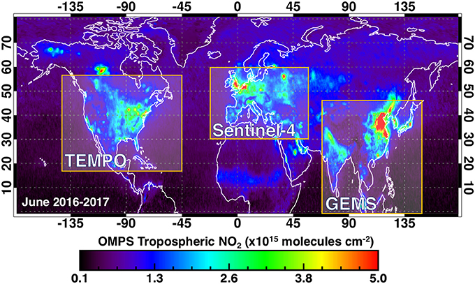
Figure 1. Global map of OMPS NM tropospheric NO₂ vertical columns for June 2016 and June 2017 averaged to 0.25° × 0.25° with the overlaid approximate spatial coverages of the planned GEO platforms: TEMPO over North America, Sentinel-4 over Europe, and GEMS over East Asia.

LEO measurements play a critical role in the global atmospheric composition constellation by providing a means of intercalibrating and cross validating the GEO sensors and by providing observations outside the fields of regard of the GEO sensors, as shown by Figure 1. The importance of the LEO component of the Global Observing System for intercalibration of LEO and GEO radiances has been recognized by the WMO-sponsored Global Space-based Intercalibration System (GSICS, http://gsics.wmo.int/), which is responsible for operational intercalibration of satellite instruments. To expand capability beyond existing activities for sensors using visible and infrared wavelengths, GSICS has initiated a UV (ultraviolet) Subgroup that focuses on cross-calibration of UV sensors, including existing LEO and future GEO instruments. Harmonizing atmospheric composition retrievals among LEO and GEO sensors is also necessary for effective utilization of the LEO and GEO measurements.

The spatial (< 10 km) and temporal (hourly) requirements for air quality measurements have largely been determined by the desire to resolve the processes affecting the emissions, lifetime and transport of tropospheric NO₂ (e.g., Beirle et al., 2011; Valin et al., 2011b, 2013; de Foy et al., 2015) because of its fundamental role in the formation of tropospheric O₃ and particulate matter. There have been a variety of approaches for validating NO₂ products retrieved from LEO platforms (e.g., Bucsela et al., 2008, 2013; Irie et al., 2008; Boersma et al., 2009; Lamsal et al., 2010; Russell et al., 2011; Travis et al., 2016). These works have identified and addressed gaps in the understanding of NO₂ retrievals, including methods for subtracting stratospheric NO₂ column contributions, a priori vertical profile deviations between urban and rural settings, and surface reflectance variations (e.g., Zhou et al., 2010; Russell et al., 2011). The additional retrieval assumptions relevant to GEO observations, for example changes in the a priori vertical profile from morning to afternoon under different solar angles or downwind of a large point source, such as a power plant, are only beginning to be assessed.

To begin addressing the spatial and temporal challenges associated with GEO measurements prior to launch, NASA funded the development of the suborbital Geostationary Trace gas and Aerosol Sensor Optimization instrument (GeoTASO, Leitch et al., 2014; Nowlan et al., 2016) and has deployed it during recent field experiments that also included networks of ground-based UV-VIS solar spectrometers (Herman et al., 2009, 2015; Pandora). Analogous to how the LEO observations are a transfer standard between the GEO domains, the airborne observations are a transfer standard between the spatial scales of the surface-based validation instruments (i.e., Pandora) and satellite observations. Here we use GeoTASO and Pandora NO₂ datasets collected as part of the KORUS-AQ study in the Seoul Metropolitan Area (SMA), South Korea during spring 2016 and as part of the NASA Student Airborne Research Program (SARP) in the Los Angeles (LA) Basin, California, USA in summer 2017 to demonstrate the spatial and temporal richness of the retrievals in anticipation of what will be routinely provided in the near-future GEO-based measurements. We frame this discussion in the context of LEO-based OMPS NM NO₂ column measurements to highlight both the spatial and temporal limitations of past datasets but also to demonstrate how LEO-platforms will continue to provide important global context to GEO-based sensors. Although field campaigns cover limited areas and time periods, these measurements provide a first taste of the air quality observations that will be measured by scheduled GEO missions at an hourly timescale by sampling repeatedly over each urban area with GeoTASO through each case study day.

Data

GeoTASO

GeoTASO is an aircraft-based UV-VIS hyperspectral imaging spectrometer built by Ball Aerospace (Leitch et al., 2014). It is being used to test air quality remote sensing retrievals for the future GEO observations from TEMPO, GEMS, and Sentinel-4. The data presented here were obtained by operating GeoTASO on the NASA LaRC UC-12B aircraft at a nominal altitude of 8.5 km. GeoTASO has two 2-dimensional CCD detectors, gathering spectral data in the visible (VIS) wavelengths (410–690 nm) and in the UV wavelengths (300–380 nm). NO₂ retrievals only use data from the VIS detector, which records spectra in one dimension (1,056 pixels) and cross-track spatial data in the second dimension (1,033 pixels). The spectral integration time is fixed at 250 ms while traveling at ground speeds of ~100–140 m/s. GeoTASO's nadir cross-track field of view is 45° providing ~7 km of cross-track coverage at altitude. Prior to the NO₂ retrieval, spectra are binned spatially to ~250 × 250 m to increase the signal-to-noise ratio.

Gapless maps were created to simulate GEO observations by flying a series of parallel flight lines spaced such that there was a small overlap between the adjacent swaths. Flight plans were developed to cover areas of 4,000–8,000 km² so that as many as four repeat measurements could be captured each day. A single traverse of this pattern across an area is referred to as a raster pattern. The urban areas in this study were mapped 3–4 times per day to simulate how the magnitude and spatial distribution of NO₂ varies diurnally at unprecedented spatial resolutions for each location. In Korea, GeoTASO data were analyzed between longitudes of 126.4 and 127.4°E and latitudes of 37.2 and 37.7°N to exclude areas outside of the SMA. Similarly, data over the LA Basin were analyzed between longitudes of −118.5 and −117.4°W and latitudes of 33.7 and 34.165°N to restrict data from outside the Basin.

Spectra from 435 to 460 nm are used to retrieve NO₂ differential slant columns (DSCs) via Differential Optical Absorption Spectroscopy (DOAS). An open-source software developed at the Royal Belgian Institute for Space Aeronomy called QDOAS (Danckaert et al., 2017) is used to compute DSCs relative to an unpolluted reference spectrum taken in flight for each region. The resulting DSC retrievals represent the total amount of NO₂ molecular absorption along the slant path of the light relative to what was present in the unpolluted reference measurement. For this study, the native resolution (250 × 250 m) DSCs are averaged to a spatial resolution of 750 × 750 m by co-adding three adjacent along-track and three adjacent across-track pixels, which is still finer than any proposed GEO or LEO satellite. This averaging decreases the average DSC error from 1.6 × 10¹⁵ molecules cm⁻² to ~5 × 10¹⁴ molecules cm⁻² and decreases the noise observed over the area of the reference spectrum (the zero baseline for these measurements) by over 50%.

The stratospheric contribution of NO₂ to the total column is small (~3 × 10¹⁵ molecules cm⁻²) and spatially uniform relative to the tropospheric DSCs observed over the SMA and the LA Basin. The temporal variation in this contribution is also small (~1 × 10¹⁴ molecules cm⁻² h⁻¹ (Sussmann et al., 2005). When retrieving DSCs from GeoTASO, the contribution of stratospheric NO₂ is observed similarly in the clean reference spectrum measurement as in all measurements, and thus is implicitly subtracted in the fitting procedure. However, time differences between the reference and retrieved observation introduces a bias in the DSCs due to the changing solar geometry altering the path length of the solar beam through the stratospheric NO₂ layer. This time-dependent bias in the stratospheric NO₂ is estimated and a correction is applied to results shown here using the solar geometry and the stratospheric NO₂ vertical column observed from OMPS NM aboard Suomi NPP (Yang et al., 2014) on the day of observation over the region of the flight. The result is a tropospheric DSC, which is henceforth shortened to TDSC. The TDSC effectively removes the largest geometric variation associated with slant columns for a typical range of solar zenith angles.

Vertical columns are typically produced by transforming retrieved slant columns using a calculated air mass factor (AMF) (Palmer et al., 2001; Lamsal et al., 2017). In a non-scattering atmosphere, the AMF reflects a simple geometric correction of the slant path of light relative to a vertical path through the atmosphere. However, in Earth's scattering atmosphere, AMF calculations require a radiative transfer model that uses solar and viewing geometry along with a priori assumptions about the vertical distribution of NO₂, surface reflectivity, and pressure. Ideally, the ancillary information used to calculate AMFs should be at a spatial resolution similar to or better than the column measurements to avoid introducing biases and artifacts (Russell et al., 2011). Datasets necessary for the AMF calculations at the sub-kilometer spatial scales of GeoTASO, including validated high-resolution chemical transport model simulations, are not yet available for the regions of interest in this work. Due to these challenges and to avoid potentially introducing spatiotemporal artifacts associated with erroneous a priori input, AMFs and vertical columns have not yet been calculated for the KORUS-AQ and SARP GeoTASO flight data. Therefore, TDSCs are shown in this work. Though the TDSC does not provide the absolute magnitude of the NO₂ column, it does provide a very good approximation for the difference in column density relative to the background represented in each region's reference spectrum. Data from GeoTASO NO₂ vertical column retrievals from the deployment in Houston, Texas in 2013 were used to assess the TDSC approximation (Nowlan et al., 2016; available at https://www-air.larc.nasa.gov/missions/discover-aq/discover-aq.html). A multiple-variable linear regression of the Houston dataset shows that 94% of the variation in vertical column is driven by the TDSC (linear coefficient of 0.85 ± 0.0002). Geometric AMF explains only about 1.7% of the variance and would not significantly alter the case study diurnal trends presented herein. The remaining variance between vertical column and TDSC, < 5%, is associated with variations in surface reflectivity and/or NO₂ vertical profile shape. Overall, the conclusions drawn in this paper are insensitive to the use of TDSC rather than tropospheric vertical column.

Pandora Spectrometer

In an effort to provide cost-effective methods for validating space-based UV-VIS trace gas measurements, including those from GEO, NASA, and ESA are collaborating on a global network of ground-based Pandora solar and sky-scanning spectrometers developed at NASA Goddard Space Flight Center (Herman et al., 2009). Pandora spectrometers are capable of retrieving accurate and precise vertical columns of NO₂ using a direct-sun DOAS technique (Herman et al., 2009). Pandora instruments are operated continuously to retrieve a NO₂ column approximately every 90 s during daylight hours, whenever the atmospheric path between the surface and the sun is cloud-free. These measurements are total NO₂ column with no differentiation of stratospheric or tropospheric NO₂ contributions, but as discussed in section GeoTASO, stratospheric contributions are relatively small and uniform over the SMA and the LA Basin. Data from these instruments have been used to assess space- and aircraft- based retrievals of NO₂ columns (Flynn et al., 2014; Nowlan et al., 2016; Goldberg et al., 2017), as well as to study the spatiotemporal variability of trace gases in urban environments (Tzortziou et al., 2015) and column-to-surface relationships and their relation to boundary layer depth (Flynn et al., 2014; Knepp et al., 2015). Further understanding the effects of boundary layer depth on air quality has been identified as a “most important” objective by the National Academy of Sciences' most recent Decadal Survey (2017–2027) (National Academies of Sciences Engineering Medicine, 2018).

This study shows NO₂ total vertical column data from three Pandoras in the SMA from May 5^th-June 15th, 2016 (Yonsei, Olympic Park and Mount Taehwa) and six Pandoras within the LA Basin from June 15^th-July 15th 2017 (UCLA, LA Main Street, Pico Rivera, CalTech, Fontana, and Ontario). For each site, 1-h averages are calculated for analysis after the data are filtered according to recommended data quality criteria (vertical column error of < 2.69 × 10¹⁴ molecules cm⁻² and normalized RMS < 0.005). Each hourly average requires at least 5 valid observations within the hour. Longer term diurnal averages (total, weekend, weekday) also calculated for analysis require over 40 valid observations per hour.

Ozone Mapping and Profiler Suite Nadir Mapper (OMPS NM)

Data from the OMPS NM hyperspectral UV instrument aboard Suomi-NPP are used to demonstrate legacy LEO measurement capability and to illustrate plans for incorporation of recently launched (TROPOMI) and future LEO missions into the air quality observing constellation. While OMI data have higher spatial resolution than OMPS NM, OMI was not operational during part of the time period of this study. OMPS NM instruments are aboard Suomi-NPP launched in 2011 and NOAA-20 launched in 2017. NO₂ is retrieved using an iterative spectral fitting algorithm at a nadir resolution of 50 × 50 km (2,500 km²) (Yang et al., 2014), which will be further improved to 17 × 17 km (289 km²) for OMPS NM aboard NOAA-20 when in its medium resolution mode (Flynn et al., 2016). OMPS NM NO₂ columns are also separated into their tropospheric and stratospheric components. The measurement precision of tropospheric NO₂ vertical column is estimated to be 3 × 10¹⁴ molecules cm⁻² (Yang et al., 2014). For this analysis, both tropospheric and stratospheric columns are used from the instrument aboard Suomi-NPP, with the latter helping correct the offset in GeoTASO's TDSCs due to the stratospheric NO₂ layer as described in the GeoTASO section. Data from OMPS NM are filtered for cloud fractions >25%.

Results and Discussion

To demonstrate the capability and limitations of currently available data, Figure 2 shows single-overpass and monthly-averaged OMPS NM NO₂ column measurements over South Korea and California. On June 9, 2016, the OMPS NM nadir overpass was to the west of the SMA. Because of the viewing geometry and the curvature of the Earth, the OMPS NM off-nadir detector elements that view the SMA cover twice as much surface area as those at nadir (nominally 50 × 50 km) on this day (Figure 2A). On the other hand, the OMPS NM nadir overpass was directly over Southern California on June 27th, 2017 (Figure 2B), such that OMPS NM was able to measure the tropospheric NO₂ column over LA near its finest spatial resolution.

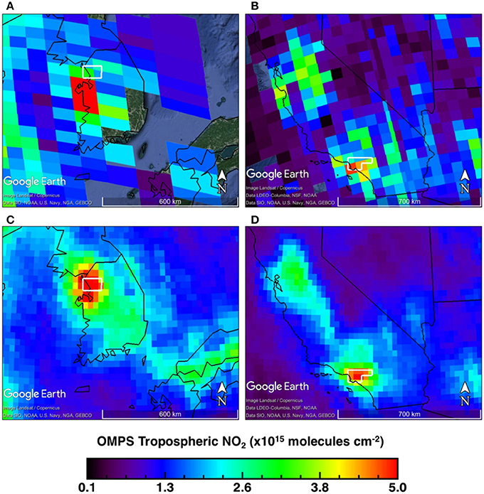
Figure 2. Tropospheric NO₂ data from OMPS NM aboard Suomi-NPP for single overpasses on (A) June 9th 2016 over South Korea and (B) June 27th, 2017 over California. The monthly averaged 0.25° × 0.25° tropospheric NO₂ from OMPS NM is shown for (C) June 2016 over South Korea and (D) June 2017 over California. White polygons in each map outline the area of the GeoTASO flights.

LEO observations can be refined spatially by “oversampling” over a longer temporal range, as the orbital track varies day-to-day leading to variable spatial sampling (e.g., the edge of swath over Korea on June 9th, 2016 vs. the nadir observations over California from June 27th, 2017). This technique has been applied to trace-gas retrievals from imaging spectrometers, like OMI, for NO₂, HCHO, and SO₂ data to identify and investigate pollution emitting sources, their average plume extent, and emission rates (de Foy et al., 2009; Russell et al., 2010; McLinden et al., 2012; Zhu et al., 2014). Figures 2C,D show the 0.25° × 0.25° (~20 × 30 km at 35°N) monthly average created by oversampling OMPS NM NO₂ data for June 2016 over South Korea (Figure 2C) and June 2017 over California (Figure 2D). Here, the OMPS NM average measurements show that NO₂ columns are locally maximum over the SMA and the LA Basin in each respective region. By providing the means to distinguish sources, long-term trends can be used to evaluate the changes of emissions driven by regulatory programs (Kim et al., 2006), technological controls (e.g., Russell et al., 2012), and economic activity (e.g., Russell et al., 2012; de Foy et al., 2016; Duncan et al., 2016). Whether considering daily measurements or analysis of long term monthly averages, instruments like OMPS NM provide a well-characterized, quantitatively stable measurement reflecting a balance of NO₂ emissions and removal at spatial scales of ~25 km, with some limited information on pollutant transport (e.g., Beirle et al., 2011; Valin et al., 2013, 2014; de Foy et al., 2016). As such, the measurements available from the past have not been sufficient to address the more pressing air quality management needs: the ability to distinguish sources within urban airsheds, characterization of local mesoscale flow patterns on pollutant transport, quantification of NO₂ removal mechanisms (e.g., Valin et al., 2013), or better characterization of photochemical ozone production to NO_x (NO + NO₂) or VOC control strategies (e.g., Martin et al., 2004; Duncan et al., 2010; Jin et al., 2017; Schroeder et al., 2017).

The LEO-based data in Figures 1, 2 represent the standard measurement that has been available to observe pollutants globally from space-based platforms for more than two decades. While finer scale global LEO data will soon be available with the addition of TROPOMI and NOAA-20 OMPS NM, the following two case studies demonstrate the information that will be gained in adding temporally resolved GEO observations to this global observing system by focusing on GeoTASO and Pandora measurements within the SMA and the LA Basin in June 2016 and 2017, respectively. Figure 3 shows maps of each metropolitan area discussed in these case studies. The white polygons encompass the area observed by GeoTASO, white stars and labels are Pandora locations, red/blue lines are major roadways (SEDAC (NASA Socioeconomic Data Applications Center) Center for International Earth Science Information Network - CIESIN - Columbia University, 2013), and icons and regions labeled in yellow are discussed in the case studies below. Areas of elevated terrain appear darker than the surrounding valleys and are typically free of strong emission sources. Densely urbanized areas within the valleys appear grayer in color. Using this map as a reference will help guide the discussion below.

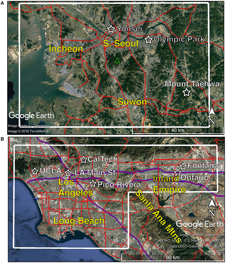
Figure 3. Maps of (A) the SMA and (B) the LA Basin. Major roads (SEDAC (NASA Socioeconomic Data Applications Center) Center for International Earth Science Information Network - CIESIN - Columbia University, 2013) are drawn in red with I-5, I-10, and CA-60 outlined in blue in (B). Pandora sites are labeled with white star icons, and regions discussed in the paper are labeled in yellow. The green triangle in the SMA is Mount Gwanaksan, and the airplane icon in the LA Basin depicts the location of LAX. GeoTASO rasters cover the approximate area depicted by the white polygons.

Case Study 1: Seoul Metropolitan Area, South Korea

The first execution of diurnal mapping over an urban area with GeoTASO was during the DISCOVER-AQ Front Range field study in summer 2014 (Crawford et al., 2016). This same strategy was used more extensively during the KORUS-AQ field study in spring 2016 (https://www-air.larc.nasa.gov/missions/korus-aq/). Figure 4 shows maps of NO₂ TDSC obtained by GeoTASO on June 9, 2016, at four different times of day between 08:00 and 18:00 LT over the SMA. Each of the four rasters cover an area of ~40 × 70 km in ~2 h. This is also the approximate area of a single nadir OMPS NM pixel (Figure 2). Overlaid in panels A,C in Figure 4 are wind vectors averaged over the lowest 500 m above ground level from the full spectral resolution (~13-km) Global Data Assimilation System (GDAS) analyses for 00:00 UTC (09:00 LT) and 06:00 UTC (15:00 LT), respectively (Kleist and Ide, 2015a,b). GDAS output, archived at 6-h intervals, is not available during the other two rasters.

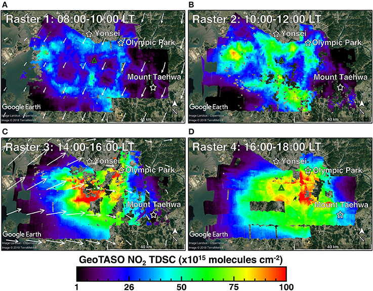
Figure 4. Maps of GeoTASO NO₂ TDSCs over SMA on June 9th, 2016 for (A) Raster 1 from 08:00 to 10:00 LT, (B) Raster 2 from 10:00 to 12:00 LT, (C) Raster 3 from 14:00 to 16:00 LT, and (D) Raster 4 from 16:00 to 18:00 LT. Pandora sites are labeled with white star icons. Rasters 1 and 3 includes wind vectors (white arrows) averaged through the lowest 500 m above ground level from the full resolution Global Data Assimilation System (GDAS) at (A) 00:00 UTC (09:00 LT) and (C) 06:00 UTC (15:00 LT).

Figure 5 shows percentile distributions of NO₂ TDSCs for each SMA raster shown in Figure 4. Over the SMA area on this day, NO₂ pollution is at its minimum in the morning then increases and becomes more variable throughout the day, demonstrating the accumulation of NO₂ at a rate faster than its removal. The area median more than doubles from 20 × 10¹⁵ molecules cm⁻² to 49 × 10¹⁵ molecules cm⁻² over the course of the day with the interquartile range (representing the variability) expanding as well. There is not a significant change in the median from late morning to mid-afternoon, however the distribution is skewed upwards with the 75th percentile reaching 58 × 10¹⁵ molecules cm⁻² for Raster 3. Raster 4 exhibits the largest magnitude and variability of NO₂ columns on June 9th with the median TDSCs approaching 50 × 10¹⁵ molecules cm⁻² and an interquartile range of 44 × 10¹⁵ molecules cm⁻². Maximum TDSCs observed over the SMA during this day, up to 120 × 10¹⁵ molecules cm⁻² and well exceeding the 95th percentile, occurred during Rasters 3 and 4.

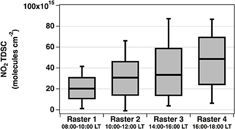
Figure 5. Box plots showing the percentile distributions of NO₂ TDSCs for each raster in SMA from Figure 4. The shaded box shows 25th−75th percentile range with the whiskers extending to the 5th and 95th percentiles. The solid line dividing each shaded box is the median.

During the morning (Rasters 1 and 2), distinct patterns are apparent with maximum NO₂ TDSCs over urbanized valleys and minimums located directly over elevated terrain. The western minimum (located south-southeast of Incheon) is not due to elevated terrain, but instead due to the lack of large emission sources within this rural farmland region. The largest TDSCs in the morning coincide with the areas with the largest temporal growth between Raster 1 and Raster 2, including Incheon, south central Seoul, and Suwon, where the TDSCs grow to a magnitude outside of the interquartile range. These are areas with dense urbanization shown in Figure 3 and are likely the areas with the largest emissions in this domain.

The morning patterns reflect emission sources (i.e., roads and urban centers) that are confined spatially. However, the spatial distribution of NO₂ TDSCs in the afternoon changes dramatically. The boundary layer grows through the day due to surface heating and, from Raster 2 to Raster 3, grows deep enough to encompass the surrounding terrain. By the afternoon it appears the mixed layer is deep enough and advection is fast enough that the spatial pattern of NO₂ columns no longer reflects the distinct pattern of emission sources. While muted in a deeper afternoon mixed layer, the terrain influence on the spatial pattern of NO₂ columns is still visible in Raster 4, where there is a local minimum in the middle of the SMA plume with a magnitude of ~70 × 10¹⁵ molecules cm⁻² near Mt. Gwanaksan (green triangle in Figures 3, 4). Over the nearby valley (5 km west), NO₂ TDSC values are 20 × 10¹⁵ molecules cm⁻² larger. There is approximately a 400 m change in elevation between these two areas. This change in NO₂ column between the mountain and the valley could be associated with either a decrease in surface concentration or a loss of volume through the column. In this case, 20 × 10¹⁵ molecules cm⁻² would equate to an average mixing ratio of 20 ppbv within the 400 m between the valley floor and the elevated terrain (assuming a temperature of 300 K and surface pressure of 1,000 hPa). This mixing ratio estimate of 20 ppbv compares well with the mixing ratios measured nearby by NCAR's 4-channel chemiluminescence instrument aboard the NASA DC-8 aircraft on this afternoon during a KORUS-AQ flight (not shown). In such situations, local minima in column amounts may not correlate with minima in surface concentrations. GEO observations, Pandora measurements, and routine air quality monitoring networks will begin to resolve some of these differences in areas with complex terrain and provide insight for similar locations without surface monitoring.

While NO₂ over the SMA generally accumulates throughout the day, this is not true for all locations within the region. On June 9th, 2016, winds from the GDAS analyses near the SMA shift from weak northerly flow in the morning (00:00 UTC−09:00 LT) to stronger anti-cyclonic westerly to southwesterly flow during the afternoon (06:00 UTC−15:00 LT). The spatial pattern over the SMA does not change from Raster 1 to Raster 2. However, during the afternoon there is a shift progressively to the east between Rasters 3 and 4, indicative of horizontal transport. This is most apparent by observing the edges of the SMA NO₂ TDSC plume, such as at Incheon where there is significant growth between Rasters 1 and 2 followed by decay and/or extension toward the east during the afternoon rasters. It takes ~2 h to cover the area of the domain in each Raster. In Raster 3, the spatial offset in TDSCs between successive overpasses (ranging from 15 to 30 min) between Incheon and south Seoul is likely caused by advection of the plume between Raster line samples. On the eastern side of the domain, the Mount Taehwa area is relatively unpolluted during Rasters 1 and 2, but between Raster 3 and Raster 4, NO₂ TDSCs increase and are consistent with what would be expected from the advection of the SMA plume to southeast based on the 15:00 LT winds.

As part of efforts to demonstrate GEO validation plans, Pandora instruments provided direct-sun vertical column NO₂ measurements that are complementary to the GeoTASO backscatter TDSCs at three sites in the SMA region (Figure 6). The selected sites cover a range of air quality conditions across the SMA, spanning the domain of GeoTASO observations from the northwest (Yonsei is just outside the raster domain due to airspace restrictions) to the east-southeast over Olympic Park and Mount Taehwa another 40 km southeast (stars in Figures 2, 4). Gray lines in Figure 6 show the hourly-averaged diurnal pattern for all days between May 5th and June 15th, 2016, with the day of the GeoTASO observations, June 9th, highlighted in red. On June 9, 2016, the observations at these sites are broadly consistent with the NO₂ column growth and transport patterns observed by GeoTASO; NO₂ columns are large and growing over low-lying population centers during the morning hours (e.g., Yonsei and Olympic Park) followed by transport to the southeast, such that columns diminish over Yonsei in the early afternoon while growing over Olympic Park briefly (also seen in Raster 3 from GeoTASO: Figure 4C) before finally diminishing over Olympic Park and growing over Taehwa in the late afternoon. At Yonsei University, Pandora measurements were made from the top of a campus building (180 m above sea level, ~130 m above ground level). As a result, observations at Yonsei University are biased low at all times of the day, especially in the morning hours, when the unsampled portion of the boundary layer (130 m) is a larger component of the typically shallower NO₂ mixing depth. A similar bias has been observed and quantified for previous Pandora measurements in Houston using coincident NO₂ in situ measurements (Judd, 2016; Nowlan et al., 2016), however this potential bias does not change the larger conclusions made here.

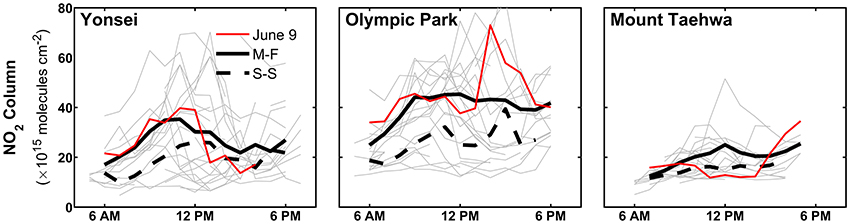
Figure 6. Hourly averaged NO₂ vertical columns observed by ground-based Pandora spectrometers at Yonsei University, Olympic Park, and Mount Taehwa. Gray lines are the individual day diurnal averages from May 5th through June 15th, 2016. June 9th, 2016 is overlaid in red, the weekday (Monday–Friday) averages are the black solid lines, and weekend (Saturday–Sunday) average observations are the black dashed lines.

June 9th, 2016 was the only day that GeoTASO was used to acquire observations at four different times throughout the day during KORUS-AQ. However, the Pandora measurements show large day-to-day variations of NO₂ column at these sites across the SMA (Figure 6, gray lines), particularly over the urban sites of Yonsei and Olympic Park, but also over the rural Mount Taehwa site, downwind of Seoul. The hourly and daily variations of NO₂ column can provide important constraints on transport models, particularly when influences from orographic and land-ocean circulations are challenging to accurately simulate.

The hourly values from Figure 6 are also averaged to calculate the weekday diurnal average in solid black and weekend average in dashed black. At all sites, the weekend column densities are lower than those during the weekdays, highlighting the influence of anthropogenic activity on air quality. The longer-term averages of the NO₂ column reveal important information on chemical transport, but primarily reveal important lessons for understanding the chemical mass balance of NO₂ emissions and loss, or insights on the importance of sources of pollutant emissions that are known to have a day-of-week variation (e.g., Beirle et al., 2003; Harley et al., 2005; Valin et al., 2014).

The magnitude of NO₂ observed in the most polluted regions of the SMA by both Pandora and GeoTASO is over an order of magnitude larger than observed by OMPS NM (Figure 2). The LEO observations roughly coincide with the time of Raster 3 in the SMA. At Olympic Park at this time, Pandora and GeoTASO both measured spikes in the local NO₂ column at the same order of magnitude (70–80 × 10¹⁵ molecules cm⁻²) and the SMA as a whole had a median of 33 × 10¹⁵ molecules cm⁻². The order of magnitude discrepancy between the finer scale measurements (GeoTASO and Pandora) and the coarse LEO observations (OMPS NM) reflect spatial averaging of over an area that also includes less NO₂-polluted air. The SMA is observed by four OMPS NM pixels, each averaging only a fraction of the enhanced NO₂ columns over the SMA with a larger area of background NO₂ columns. Only moderate enhancements (~3 × 10¹⁵ molecule cm⁻²) are observed over the SMA by the ~20,000 km² covered by the four OMPS NM pixels. Looking at the oversampled monthly averaged data (Figure 2C), the spatial patterns correlate better with those observed by GeoTASO observations with a peak centered over the SMA region. Over this month there are fewer polluted days than the case shown on June 9th, as shown by the Pandora measurements in Figure 6, resulting in a smaller magnitude of NO₂ over the SMA on the month time-scale vs. the afternoon sample from Raster 3. Comparisons of OMPS NM data (50 × 50 km) with OMI data (24 × 13 km) (Yang et al., 2014) and OMI operational products with super-zoom OMI data (~7 × 13 km; Valin et al., 2011a) confirm that neither OMPS NM nor OMI operational footprints are sufficient to resolve the small-scale NO₂ spatial variations over localized sources. Due to the nature of NO₂ emissions and its short atmospheric lifetime, air quality applications require that the variability of NO₂ columns are spatially resolved (e.g., Cohan et al., 2006; Valin et al., 2011b), a capability anticipated from future LEO (TROPOMI: 3.5 × 7 km) and GEO platforms.

Case Study 2: Los Angeles Basin, California

Figure 7 shows NO₂ TDSC maps obtained over the LA Basin at three different times on June 27th, 2017, capturing the morning, mid-day, and late afternoon periods. The left column shows the 750 × 750 m resolution TDSCs from GeoTASO and the right column shows a product that is co-added to 3 × 3 km to emulate a sampling footprint that is more comparable to what is anticipated from GEO. The area of this raster spans ~50 × 50 km in the southern half and ~115 km east-to-west on the northern side of the Basin. Overlaid are boundary layer averaged wind vectors from the North American Model (NAM)-CONUS 3-km nest (Janjic and Gall, 2012) from 16:00 UTC (09:00 LT) on Raster 1, 20:00 UTC (13:00 LT) on Raster 2, and 00:00 UTC (17:00 LT) for Raster 3. Figure 8 shows percentile distributions of NO₂ TDSCs for each LA Raster at the 750 × 750 m resolution (the left column of Figure 7). Maximum NO₂ columns are observed in the morning, with a median NO₂ TDSC over the LA Basin of 12.5 × 10¹⁵ molecules cm⁻² during Raster 1. The median value decreases ~50% between the morning and late afternoon (Raster 1 vs. Raster 3) in the LA Basin.

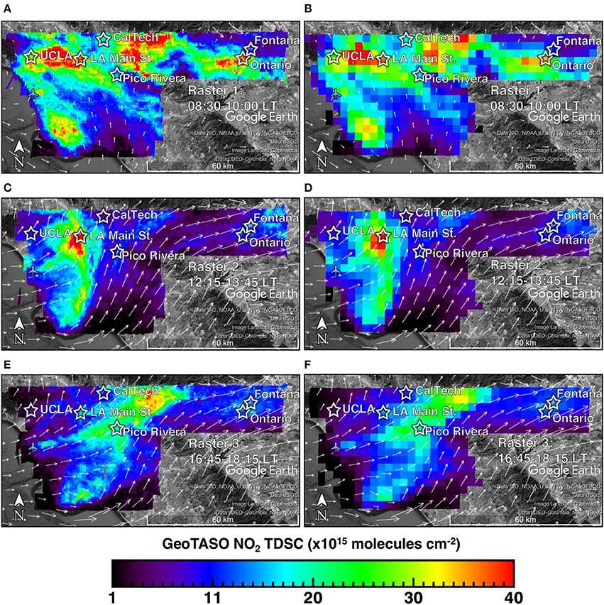
Figure 7. Maps of GeoTASO NO₂ TDSCs over the LA Basin on June 27th, 2017. Raster 1 from 08:30 to 10:00 LT is shown in (A,B), Raster 2 from 12:15 to 13:45 LT is shown in (C,D), and Raster 3 from 16:45 to 18:15 LT is shown in (E,F). Panels (A,C,E) are at 750 × 750 m resolution, whereas (B,D,F) are the TDSCs binned to 3 × 3 km spatial resolution. Overlaid are the boundary layer averaged wind vectors (white arrows) from the NAM-CONUS 3-km nest analysis for 16:00 UTC (09:00 LT) in (A,B), 20:00 UTC (13:00 LT) in (C,D), and 00:00 UTC (17:00 LT) in (E,F).

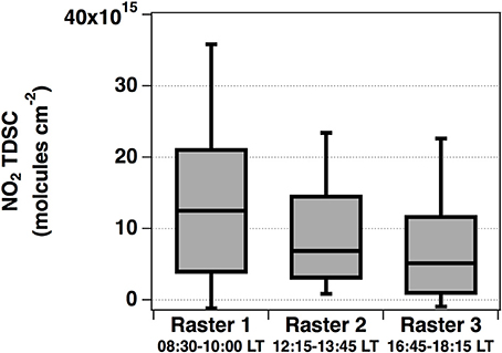
Figure 8. Box plots showing the percentile distributions of NO₂ TDSCs for each raster in the LA Basin from Figure 7. The shaded box shows 25th−75th percentile range with the whiskers extending to the 5th and 95th percentiles. The solid line dividing each shaded box is the median.

Winds are relatively light in the morning and the spatial distribution of NO₂ is consistent with the distribution of emission sources. During Raster 1, enhancements that likely reflect mobile emission sources are located over freeways (e.g., I10, I5, and CA60: blue outlined roads in Figure 3) with the largest enhancements over downtown Los Angeles (just west of LA Main Street) where many of these freeways intersect and traffic congestion could lead to local emission enhancements. An additional maximum is observed over Los Angeles International Airport (LAX) on the coast (airplane icon in Figure 3), a large NO_x emission source. The lowest columns measured coincide with areas of elevated terrain, such as the hills west of Long Beach, and areas of the Santa Ana Mountains.

On the western side of the Basin during Raster 2, GeoTASO observes a line of high NO₂ TDSCs with the appearance of a frontal structure, extending north-to-south from Glendale down to Long Beach, peaking near downtown Los Angeles. Also, the hot spot observed over LAX during Raster 1 is now more diffuse with a plume-like structure extending to the east, indicative of horizontal transport inland. With the LA Basin's location on the Pacific Coast, the area is often influenced by mesoscale land/water circulations (i.e., sea breezes) due to unequal heating over the land and water, which could result in eastward transport of pollution within the LA Basin during the daytime. Figure 9 illustrates the role of sea breeze transport on this day. Figure 9A shows contoured 2-meter relative humidity (RH) and boundary layer averaged wind vectors from the NAM-CONUS 3-km nest over the western half of the LA Basin at 20:00 UTC (13:00 LT: the midpoint time of Raster 2). On this map, the largest gradient in relative humidity and shift in wind vectors occurs around the 40% relative humidity contour indicating the boundary between the land and marine air masses (i.e., the sea breeze front). The 40% contours from 19:00, 20:00, and 21:00 UTC are overlaid on the GeoTASO NO₂ TDSCs from Raster 2 in Figure 9B to indicate the movement of the sea breeze front during Raster 2 in relation to the NO₂ feature observed during this time. These modeled results are similar in timing to the observed sea breeze arrival at the South Coast Air Quality Monitoring District's LA Main Street monitoring location, which saw an air mass transition at 13:30 LT with a slow increase in westerly wind speed and a 10% increase in RH. The edge of the peninsula to the west of Long Beach has hilly terrain that acts as a barrier to the penetrating sea breeze front, and due to the orientation of the coastline in this area, there are two different sea breeze fronts pushing inland and converging around the Long Beach area. The spatial structure of NO₂ during Raster 2 mimics the shape of the sea breeze front that is pushing inland, suggesting that this front is advecting the pollution that was along the coast to the east as the marine air mass progresses inland through the afternoon. In fact, it appears that NO₂ is confined within the convergence zone between the two sea breeze fronts in the southern end of the Raster. The influence of air mass convergence on pollution build up has been observed in other coastal regions, such as in Houston, Texas, where synoptically driven offshore flow can converge with the sea breeze front allowing for the buildup of pollution within its convergence zone and causing poor air quality (Banta et al., 2005). Although less defined, this linear NO₂ feature within the continued presence of the convergence zone also appears in Raster 3 (Figure 7E) slightly further to the east, demonstrating the influence of this convergence zone over the duration of the afternoon.

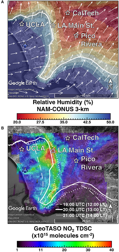
Figure 9. (A) Relative humidity from the NAM-CONUS 3-km nest at 20:00 UTC (13:00 LT) with overlaid modeled boundary layer averaged wind vectors and a white contour at 40% relative humidity boundary indicating the sea breeze front position and (B) NO₂ TDSCs over the western side of the LA Basin during Raster 2 with the indicated sea breeze front position identified from the NAM-CONUS 3-km nest 40% relative humidity contour at 19:00UTC (long dashes: 12:00 LT), 20:00UTC (solid: 13:00 LT), and 21:00UTC (dotted: 14:00 LT).

The appearance of enhanced NO₂ during Raster 3 between downtown Los Angeles and the Inland Empire coincides with an area of enhancement also observed during the morning flight. It is impossible to tell from the available data in this study whether this enhancement is due to continued sea breeze transport or the result of increased local emissions during the late afternoon, but as a whole, these datasets demonstrate the complexity of the spatial distribution of NO₂ in a coastal urban metropolitan surrounded by complex terrain.

To provide an initial assessment of the data that will be routinely available from GEO observations, the LA Basin data are binned up to 9 km² (expected nadir areal resolution of TEMPO; Zoogman et al., 2017) by averaging the data into 3 × 3 km pixel bins (Figure 7 right). While the signatures are muted due to spatial averaging, the features discussed in the preceding paragraphs remain spatially distinct, demonstrating how GEO observations from TEMPO are expected to address salient air quality questions, even in a coastal region with complex terrain, mesoscale circulations, and highly variable emission patterns.

Figure 10 is the same format as Figure 6, but for the six Pandoras installed in the LA Basin, showing data between the dates of June 15th and July 15th, 2017. Pandora NO₂ vertical column measurements in the LA Basin on June 27th, 2017 (Figure 10: red lines) are broadly consistent with the NO₂ column growth and transport patterns observed by GeoTASO, most notably the early afternoon peak at LA Main Street coinciding with the sea breeze front arrival on this day. NO₂ columns observed by Pandora spectrometers are generally at a maximum in the mid-morning hours and decrease in the early afternoon hours on weekdays. Over coastal and downtown Los Angeles sites (UCLA, LA Main Street), NO₂ columns continue to decrease or remain steady in the late afternoon hours whereas NO₂ columns grow at Pico Rivera, Ontario, and Fontana, reflecting the inland transport of cleaner air at the coast and more polluted air at the downwind sites in the presence of westerly prevailing winds.

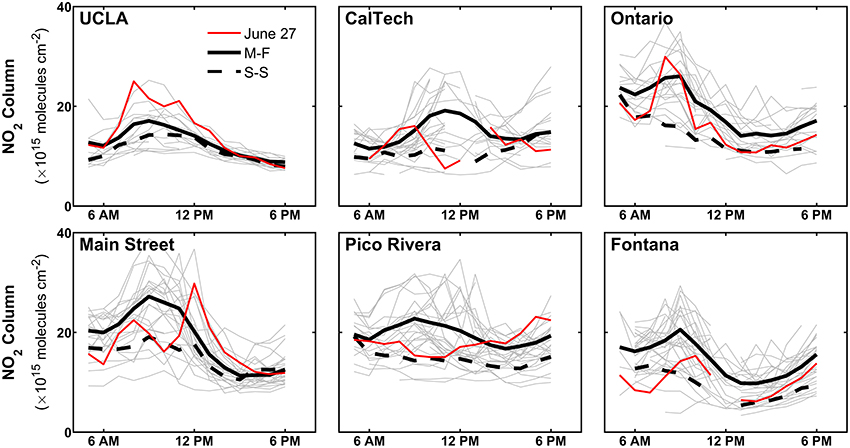
Figure 10. Hourly averaged NO₂ vertical columns observed by ground-based Pandora spectrometers at UCLA, Los Angeles Main Street, CalTech, Pico Rivera, Ontario and Fontana. Gray lines are the individual day diurnal averages from June 15th through July 15th, 2017. June 27th, 2017 is overlaid in red, the weekday (Monday–Friday) averages are the black solid lines, and weekend (Saturday–Sunday) average observations are the black dashed lines.

While the overlying diurnal features are apparent on many days (e.g., the morning peak in NO₂ at most sites), day-to-day variability in Pandora data (Figure 10: gray lines) shows significant deviation from the average patterns. For example, the sea breeze front that shows a distinct maximum over LA Main Street on June 27th only occurs on a handful of other days that month. CalTech is also different from the other sites in that its NO₂ peak is around midday. CalTech is not a primary NO₂ source area, but instead a potential receptor for Los Angeles's early morning emissions under the right transport conditions (not seen on June 27th). Additionally, CalTech is ~250 m above sea level (or about 150 m higher than the LA Main Street site) and another midday contributor there may be mixing from lower-lying areas to the elevation sampled by the Pandora as the mixed layer grows throughout the day. NO₂ columns are smaller at all sites on the weekend (Saturday–Sunday) than during the week (Monday–Friday), with a few sites exhibiting flat-shaped weekend temporal profiles, indicating minimal change in column throughout the weekend day (CalTech, Pico Rivera).

The near-nadir measurements over the LA Basin from OMPS NM on June 27th, 2017 (Figure 2B: 2–5 × 10¹⁵ molecules cm⁻²) have a similar order of magnitude as the midday GeoTASO measurements during Raster 2 (median of 6.8 × 10¹⁵ molecules cm⁻²). The area covered by GeoTASO is ~1.5 times the area of a nadir OMPS NM pixel, but the GeoTASO raster does not encompass any single OMPS NM pixel in its entirety from this overpass in which to do a one-to-one comparison. However, the oversampled image (Figure 2D) does suggest that over a month-long timescale, OMPS NM observes NO₂ confined to the area measured by GeoTASO within the LA Basin at the same order of magnitude as this GeoTASO case study day.

Case Study Comparative Discussion

While these case studies did not occur simultaneously and were in two different urbanized regions, both examples were taken during weekdays in June with minimal cloud impact and the same repeated sampling strategy to simulate future observations from GEO platforms. The Pandora data expand these studies to a broader late spring/early summer temporal coverage to extend the analysis beyond the single days of GeoTASO data shown. Similarities and differences between the measurements in these two case studies illustrate opportunities for future analysis in comparing and contrasting spatiotemporal trends in different regions. Here, we discuss qualitative comparative findings between the two different urbanized regions of the SMA and the LA Basin.

Meteorologically, these 2 flight days have similarities in near-surface dynamics between the morning and afternoon. In the early morning, the winds are relatively light in each region and the spatial distribution of NO₂ is consistent with known large emission sources: urbanized valleys within the SMA and freeways and LAX in the LA Basin. Later in the day, dynamics have a stronger role in determining the spatial patterns associated with NO₂ in both areas. The anti-cyclonic flow that develops in the SMA pushes the large urban plume to the west then southwest and over the receptor site of Mount Taehwa, consistent with Pandora observations on this day and many other days during the late-spring period. In the LA Basin, a sea breeze front pushes enhanced NO₂ columns inland near midday and continues into the early evening observations. Due to the topography and orientation of the coast, the sea breeze front advances inland from different directions and converges, advecting, and then containing NO₂ within this convergence zone.

Pandora data demonstrate the complexity of day-to-day variability associated with variations in meteorology and anthropogenic emission patterns. While this work does not expand the meteorological analysis beyond GeoTASO flight days, these datasets shows how the magnitude of the column changes depending on the day-of-week. NO₂ columns are smaller at all sites on the weekend (Saturday–Sunday) than during the week (Monday–Friday) in both regions. These weekday-weekend differences are a fingerprint that can help identify the contribution of various anthropogenic NO₂ sources based on our understanding of their day-of-week variation (e.g., heavy duty diesel trucking; Harley et al., 2005) and important non-linear chemical feedbacks (e.g, Valin et al., 2014).

These two urban areas exhibit contrasting diurnal patterns during the two GeoTASO flight days. On June 9th, 2016, NO₂ constantly accumulates in the SMA, whereas in the LA Basin on June 27th, 2017, NO₂ is largest during the mid-morning Raster and then decreases in the afternoon/early evening. In the SMA, this trend of NO₂ increasing throughout the day sometimes, but not always, occurs over the individual Pandora sites of Yonsei and Olympic Park and is often driven by very large hour-to-hour variations in the column. In the LA Basin, the mid-morning peak in NO₂ columns followed by decreases during the afternoon is a common pattern that shows up frequently in the day-to-day observations from Pandora at most sites, with the exception of the CalTech site which shows peak NO₂ slightly later in the day. The differing diurnal pattern observed by GeoTASO on these days may indicate more prevalent mid-day sources in the SMA relative to the LA Basin, differing chemistry regimes, or perhaps just a difference in transport patterns during the case study periods. With GEO platforms providing more data to test these hypotheses over these and many more urban areas, we anticipate exciting opportunities for future air quality research.

Conclusions

This work illustrates the spatiotemporal detail that will be resolved with the upcoming GEO air quality measurements, using GeoTASO NO₂ retrievals as a proxy, and how ground-based and LEO datasets will play important roles in validating and connecting these GEO observations from the local- to global-scale. Data from GeoTASO, used as a testbed to address GEO validation needs and to anticipate future opportunities for air quality management applications, is used to resolve the spatiotemporal patterns of NO₂ TDSCs over the SMA and LA Basin. In the morning, under the influence of weak winds, spatial patterns of NO₂ reflect the spatial distribution of emission sources and topography over the SMA and the LA Basin. NO₂ column densities over the SMA grow throughout the day on June 9th, 2016 as emission rates outweigh NO₂ removal from the column, while on June 27th, 2017, NO₂ in the LA Basin peaks during the mid-morning hours indicating that removal processes overtake emission rates before midday. GEO observations will show whether these conclusions apply beyond the case studies shown here, as well as expanding to other metropolitan areas around the globe. These spatially and temporally refined measurements will begin to link the role of emissions and atmospheric dynamics with the spatial distribution of pollutants in regions impacted by poor air quality, details that past LEO observations were incapable of capturing.

In addition to the single day of GeoTASO data analyzed for each case study region, Pandora observations demonstrate day-to-day and hour-to-hour variability of NO₂ that will be measured from GEO and provide a means of linking the satellite-based column measurements to variations in surface concentrations. Over both the SMA and the LA Basin, Pandora measurements reveal that NO₂ columns vary between weekdays and weekends and between source and receptor sites. They also fluctuate greatly on a day-to-day basis from the statistically calculated diurnal averages, particularly near large sources. The frequent Pandora observations, many times per hour, and their anticipated co-location with surface air quality and meteorology monitoring instrumentation will also provide insight to transient local processes that better inform the use of column-integrated measurements for monitoring surface-based pollution.

LEO-based datasets will be essential for intercalibrating radiances measured by each of the GEO instruments as well as cross-validating their data products. Observations from decades of LEO observations have provided compelling verification of multi-year changes in pollutant emissions in different regions of the world. While unavailable during the presented case studies, LEO observations are now attaining similar spatial resolutions as those expected from the GEO instruments with the addition of TROPOMI. As illustrated by these case studies, pollutant concentrations vary greatly through the day, particularly in urban areas. Variations are driven by factors that also change through the day: emissions, photochemistry, and meteorology. Sparse observations, including temporally sparse LEO observations (e.g., OMPS NM) and spatially sparse surface measurements (e.g., Pandora), do not permit these factors to be disentangled, limiting improvements in air quality assessment and prediction. The GeoTASO data shown in these case studies illustrate one change in perspective the GEO observations will provide: moving beyond coarse, static early-afternoon snapshots from LEO to dynamic visualization of chemical weather. Together the pieces of this system will enable better understanding of the locations and magnitudes of emissions and of meteorological influences, better monitoring of the air we breathe, and ultimately more effective strategies for improving air quality.

Data Availability

• GeoTASO data can be provided upon request and will become publicly available after August 2018 on the KORUS-AQ data archive (https://www-air.larc.nasa.gov/cgi-bin/ArcView/korusaq?B200=1) and the LMOS archive (https://www-air.larc.nasa.gov/cgi-bin/ArcView/lmos). GeoTASO data from DISCOVER-AQ Texas used in the TDSC justification can be found at https://www-air.larc.nasa.gov/missions/discover-aq/discover-aq.html.

• Pandora data are available on data.pandonia.net

• OMPS NM data are available at https://doi.org/10.5067/N0XVLE2QAVR3

• GFS and NAM meteorology are available at http://nomads.ncep.noaa.gov/

• SCAQMD hourly meteorology data is available https://www.arb.ca.gov/aqmis2/metselect.php, and higher temporal resolution is available upon request from SCAQMD.

Author Contributions

LJ, JA-S, and RP formulated the central research idea. LJ and JA-S drafted the manuscript. LJ led the processing and analysis of GeoTASO data with the help of SJ for retrieving NO₂ DSCs for SMA. MT and MM calibrated and processed the Pandora NO₂ retrievals and LV led Pandora data analysis. RP provided the modeled meteorology dataset and relevant processing scripts. KY provided OMPS NM data. JS was involved with Pandora measurements and maintenance in South Korea. SJ, MK, and JA-S participated in the flight planning and data gathering during GeoTASO flights in South Korea, with the addition of LJ in California. All authors provided input, suggestions, and edits to the manuscript.

Funding

This work was partly funded by NASA Earth Science Division's GEOCAPE Mission Study, NASA Tropospheric Composition Program, and the EPA National Exposure Research Laboratory. Pandora deployment, operation and the near real time processing of data were collaboratively supported by the NASA Earth Science Division funded Pandora Project team (R. Swap, PI) at GSFC in Greenbelt, MD, USA and by the ESA funded Pandonia team (A. Cede, PI) from Luftblick in Kreith, Austria. LJ's research was supported by an appointment to the NASA Postdoctoral Program at the NASA Langley Research Center, administered by Universities Space Research Association under contract with NASA. The development and production of OMPS-NM NO2 data are supported by NASA Suomi NPP science team under grant NNX14AR20A (KY, PI).

Disclaimer

The views, opinions, and findings contained in this report are those of the author(s) and should not be construed as an official National Oceanic and Atmospheric Administration, Environmental Protection Agency, or U.S. Government position, policy, or decision.

Conflict of Interest Statement

The authors declare that the research was conducted in the absence of any commercial or financial relationships that could be construed as a potential conflict of interest.

Acknowledgments

The authors extend appreciation to the South Coast Air Quality Monitoring District (SCAQMD) and our colleagues at UCLA and CalTech for providing accommodations for the Pandora Spectrometers in the LA Basin, Olga Pikelnaya for providing high temporal resolution SCAQMD in situ meteorology data, the KORUS-AQ science team, Nader Abuhassan and NASA's Pandora Project, ESA's Pandonia team, NASA SARP 2017 and NSRC, Barry Lefer from NASA Headquarters for inviting us to participate in SARP 2017, and our pilots and flight crew during both field missions.

References

Banta, R. M., Senff, C. J., Nielsen-Gammon, J., Darby, L. S., Ryerson, T. B., Alvarez, R. J., et al. (2005). A bad air day in Houston. Bull. Am. Meteorol. Soc. 86, 657–669. doi: 10.1175/BAMS-86-5-657
Beirle, S., Boersma, K. F., Platt, U., Lawrence, M. G., and Wagner, T. (2011). Megacity emissions and lifetimes of nitrogen oxides probed from space. Science 333, 1737–1739. doi: 10.1126/science.1207824
Beirle, S., Platt, U., Wenig, M., and Wagner, T. (2003). Weekly cycle of NO2 by GOME measurements: a signature of anthropogenic sources. Atmos. Chem. Phys. Discuss. 3, 3451–3467. doi: 10.5194/acpd-3-3451-2003
Boersma, K. F., Jacob, D. J., Trainic, M., Rudich, Y., DeSmedt, I., Dirksen, R., et al. (2009). Validation of urban NO2 concentrations and their diurnal and seasonal variations observed from the SCIAMACHY and OMI sensors using in situ surface measurements in Israeli cities. Atmos. Chem. Phys. 9, 3867–3879. doi: 10.5194/acp-9-3867-2009
Bovensmann, H., Burrows, J. P., Buchwitz, M., Frerick, J., Noël, S., Rozanov, V. V., et al. (1999). SCIAMACHY: mission objectives and measurement modes. J. Atmos. Sci. 56, 127–150. doi: 10.1175/1520-0469(1999)056<0127:SMOAMM>2.0.CO;2
Bucsela, E. J., Krotkov, N. A., Celarier, E. A., Lamsal, L. N., Swartz, W. H., Bhartia, P. K., et al. (2013). A new stratospheric and tropospheric NO2 retrieval algorithm for nadir-viewing satellite instruments: applications to OMI. Atmos. Meas. Tech. 6, 2607–2626. doi: 10.5194/amt-6-2607-2013
Bucsela, E. J., Perring, A. E., Cohen, R. C., Boersma, K. F., Celarier, E. A., Gleason, J. F., et al. (2008). Comparison of tropospheric NO2 from in situ aircraft measurements with near-real-time and standard product data from OMI. J. Geophys. Res. 113. doi: 10.1029/2007JD008838
Burrows, J. P., Weber, M., Buchwitz, M., Rozanov, V., Ladstätter-Weißenmayer, A., Richter, A., et al. (1999). The global ozone monitoring experiment (GOME): mission concept and first scientific results. J. Atmos. Sci. 56, 151–175. doi: 10.1175/1520-0469(1999)056<0151:TGOMEG>2.0.CO;2
Callies, J., Corpaccioli, E., Eisinger, M., Hahne, A., and Lefebvre, A. (2000). GOME-2-Metop's second-generation sensor for operational ozone monitoring. ESA Bull. 102, 28–36.
CEOS (2011). A Geostationary Satellite Constellation for Observing Global Air Quality: An International Path Forward. Available online at: http://ceos.org/document_management/Virtual_Constellations/ACC/Documents/AC-VC_Geostationary-Cx-for-Global-AQ-final_Apr2011.pdf (Accessed March 6, 2018).
Cohan, D. S., Hu, Y., and Russell, A. G. (2006). Dependence of ozone sensitivity analysis on grid resolution. Atmos. Environ. 40, 126–135. doi: 10.1016/j.atmosenv.2005.09.031
Crawford, J. H., Al-Saadi, J., Pierce, G., Long, R. W., Szykman, J. J., Leitch, J., et al. (2016). “Multi-perspective observations of NO2 over the Denver area during DISCOVER-AQ: insights for future monitoring,” in EM: Air and Waste Management Associations Magazine for Environmental Managers (Pittsburgh, PA: Air & Waste Management Association), 5.
Danckaert, T., Fayt, C., Van Roozendael, M., De Smedt, I., Letocart, V., Merlaud, A., et al. (2017). QDOAS Software User Manual. Available online at: http://uv-vis.aeronomie.be/software/QDOAS/QDOAS_manual.pdf (Accessed March 27, 2018).
de Foy, B., Krotkov, N. A., Bei, N., Herndon, S. C., Huey, L. G., Martínez, A.-P., et al. (2009). Hit from both sides: tracking industrial and volcanic plumes in Mexico City with surface measurements and OMI SO2 retrievals during the MILAGRO field campaign. Atmos. Chem. Phys. 9, 9599–9617. doi: 10.5194/acp-9-9599-2009
de Foy, B., Lu, Z., and Streets, D. G. (2016). Impacts of control strategies, the Great Recession and weekday variations on NO2 columns above North American cities. Atmos. Environ. 138, 74–86. doi: 10.1016/j.atmosenv.2016.04.038
de Foy, B., Lu, Z., Streets, D. G., Lamsal, L. N., and Duncan, B. N. (2015). Estimates of power plant NOx emissions and lifetimes from OMI NO2 satellite retrievals. Atmos. Environ. 116, 1–11. doi: 10.1016/j.atmosenv.2015.05.056
De Smedt, I., Stavrakou, T., Hendrick, F., Danckaert, T., Vlemmix, T., Pinardi, G., et al. (2015). Diurnal, seasonal and long-term variations of global formaldehyde columns inferred from combined OMI and GOME-2 observations. Atmos. Chem. Phys. Discuss. 15, 12241–12300. doi: 10.5194/acpd-15-12241-2015
Duncan, B. N., Lamsal, L. N., Thompson, A. M., Yoshida, Y., Lu, Z., Streets, D. G., et al. (2016). A space-based, high-resolution view of notable changes in urban NOx pollution around the world (2005-2014). J. Geophys. Res. Atmos. 121, 976–996. doi: 10.1002/2015JD024121
Duncan, B. N., Yoshida, Y., Olson, J. R., Sillman, S., Martin, R. V., Lamsal, L., et al. (2010). Application of OMI observations to a space-based indicator of NOx and VOC controls on surface ozone formation. Atmos. Environ. 44, 2213–2223. doi: 10.1016/j.atmosenv.2010.03.010
Fishman, J., Iraci, L. T., Al-Saadi, J., Chance, K., Chavez, F., Chin, M., et al. (2012). The United States' next generation of atmospheric composition and coastal ecosystem measurements: NASA's Geostationary Coastal and Air Pollution Events (GEO-CAPE) mission. Bull. Am. Meteorol. Soc. 93, 1547–1566. doi: 10.1175/BAMS-D-11-00201.1
Flynn, C. M., Pickering, K. E., Crawford, J. H., Lamsal, L., Krotkov, N., Herman, J., et al. (2014). Relationship between column-density and surface mixing ratio: statistical analysis of O3 and NO2 data from the July 2011 Maryland DISCOVER-AQ mission. Atmos. Environ. 92, 429–441. doi: 10.1016/j.atmosenv.2014.04.041
Flynn, L., Zhang, Z., Mikles, V., Das, B., Niu, J., Beck, C. T., et al. (2016). Algorithm Theoretical Basis Document for NOAA NDE OMPS Version 8 Total Column Ozone (V8TOz) Environmental Data Record (EDR) Version 1.0. Available online at: https://www.star.nesdis.noaa.gov/jpss/documents/ATBD/ATBD_OMPS_TC_V8TOz_v1.1.pdf (Accessed May 30, 2017).
Flynn, L. E., Homstein, J., and Hilsenrath, E. (2004). “The ozone mapping and profiler suite (OMPS). The next generation of US ozone monitoring instruments,” in 2004 IEEE International Geoscience and Remote Sensing Symposium, (Anchorage, AK: IGARSS), 155.
Goldberg, D. L., Lamsal, L. N., Loughner, C. P., Swartz, W. H., Lu, Z., and Streets, D. G. (2017). A high-resolution and observationally constrained OMI NO2 satellite retrieval. Atmos. Chem. Phys. 17, 11403–11421. doi: 10.5194/acp-17-11403-2017
Harley, R. A., Marr, L. C., Lehner, J. K., and Giddings, S. N. (2005). Changes in motor vehicle emissions on diurnal to decadal time scales and effects on atmospheric composition. Environ. Sci. Tech. 39, 5356–5362. doi: 10.1021/es048172
Herman, J., Cede, A., Spinei, E., Mount, G., Tzortziou, M., and Abuhassan, N. (2009). NO2 column amounts from ground-based Pandora and MFDOAS spectrometers using the direct-sun DOAS technique: intercomparisons and application to OMI validation. J. Geophys. Res. 114, 1–20. doi: 10.1029/2009JD011848
Herman, J., Evans, R., Cede, A., Abuhassan, N., Petropavlovskikh, I., and McConville, G. (2015). Comparison of ozone retrievals from the Pandora spectrometer system and Dobson spectrophotometer in Boulder, Colorado. Atmos. Meas. Tech. 8, 3407–3418. doi: 10.5194/amt-8-3407-2015
IGACO (2004). International Global Atmospheric Chemistry Observations Strategy Theme Report. (No. ESA SP-1282, GW No. 159, WMO TD No. 1235). Available online at: http://www.fao.org/gtos/igos/docs/IGACO-Theme-Report-2004-4.pdf (Accessed March 6, 2018).
Ingmann, P., Veihelmann, B., Langen, J., Lamarre, D., Stark, H., and Courrèges-Lacoste, G. B. (2012). Requirements for the GMES Atmosphere Service and ESA's implementation concept: Sentinels-4/-5 and−5p. Remote Sens. Environ. 120, 58–69. doi: 10.1016/j.rse.2012.01.023
Irie, H., Kanaya, Y., Akimoto, H., Tanimoto, H., Wang, Z., Gleason, J. F., et al. (2008). Validation of OMI tropospheric NO2 column data using MAX-DOAS measurements deep inside the North China Plain in June 2006: mount tai experiment 2006. Atmos. Chem. Phys. 8, 6577–6586. doi: 10.5194/acp-8-6577-2008
Jaegl,é, L., Steinberger, L., Martin, R. V., and Chance, K. (2005). Global partitioning of NOx sources using satellite observations: relative roles of fossil fuel combustion, biomass burning and soil emissions. Faraday Discuss. 130, 407–423. doi: 10.1039/b502128f
Janjic, Z., and Gall, R. (2012). Scientific Documentation of the NCEP Nonhydrostatic Multiscale Model on the B Grid (NMMB). Part 1 Dynamics. UCAR/NCAR.
Jin, X., Fiore, A. M., Murray, L. T., Valin, L. C., Lamsal, L. N., Duncan, B., et al. (2017). Evaluating a space-based indicator of surface ozone-NOx-VOC sensitivity over midlatitude source regions and application to decadal trends. J. Geophys. Res. Atmos. 122, 10–461. doi: 10.1002/2017JD026720
Judd, L. M. (2016). Investigating the Spatiotemporal Variability of NO2 and Photochemistry in Urban Areas. Dissertation. Houston, TX: University of Houston.
Kim, J., Kim, M., and Choi, M. (2017). “Monitoring aerosol properties in east asia from geostationary orbit: GOCI, MI and GEMS,” in Air Pollution in Eastern Asia: An Integrated Perspective ISSI Scientific Report Series. (Cham: Springer), 323–333.
Kim, S.-W., Heckel, A., McKeen, S. A., Frost, G. J., Hsie, E.-Y., Trainer, M. K., et al. (2006). Satellite-observed U.S. power plant NOx emission reductions and their impact on air quality. Geophys. Res. Lett. 33. doi: 10.1029/2006GL027749
Kleist, D. T., and Ide, K. (2015a). An OSSE-based evaluation of hybrid variational–ensemble data assimilation for the NCEP GFS. Part I: system description and 3D-hybrid results. Mon. Weather Rev. 143, 433–451. doi: 10.1175/MWR-D-13-00351.1
Kleist, D. T., and Ide, K. (2015b). An OSSE-based evaluation of hybrid variational–ensemble data assimilation for the NCEP GFS. Part II: 4DEnVar and hybrid variants. Mon. Weather Rev. 143, 452–470. doi: 10.1175/MWR-D-13-00350.1
Knepp, T., Pippin, M., Crawford, J., Chen, G., Szykman, J., Long, R., et al. (2015). Estimating surface NO2 and SO2 mixing ratios from fast-response total column observations and potential application to geostationary missions. J. Atmos. Chem. 72, 261–286. doi: 10.1007/s10874-013-9257-6
Lamsal, L. N., Janz, S. J., Krotkov, N. A., Pickering, K. E., Spurr, R. J. D., Kowalewski, M. G., et al. (2017). High-resolution NO2 observations from the Airborne Compact Atmospheric Mapper: retrieval and validation. J. Geophys. Res. Atmos. 122, 1953–1970. doi: 10.1002/2016jd025483
Lamsal, L. N., Martin, R. V., van Donkelaar, A., Celarier, E. A., Bucsela, E. J., Boersma, K. F., et al. (2010). Indirect validation of tropospheric nitrogen dioxide retrieved from the OMI satellite instrument: insight into the seasonal variation of nitrogen oxides at northern midlatitudes. J. Geophys. Res. 115. doi: 10.1029/2009JD013351
Leitch, J. W., Delker, T., Good, W., Ruppert, L., Murcray, F., Chance, K., et al. (2014). The GeoTASO Airborne Spectrometer Project. San Diego, CA.
Levelt, P. F., Oord, G. H. J., van den, Dobber, M. R., Malkki, A., Visser, H., Vries, J. de, et al. (2006). The ozone monitoring instrument. IEEE Trans. Geosci. Remote Sens. 44, 1093–1101. doi: 10.1109/TGRS.2006.872333
Martin, R. V., Fiore, A. M., and Van Donkelaar, A. (2004). Space-based diagnosis of surface ozone sensitivity to anthropogenic emissions. Geophys. Res. Lett. 31. doi: 10.1029/2004GL019416
Martin, R. V., Jacob, D. J., Chance, K., Kurosu, T. P., Palmer, P. I., and Evans, M. J. (2003). Global inventory of nitrogen oxide emissions constrained by space-based observations of NO2 columns. J. Geophys. Res. 108. doi: 10.1029/2003JD003453
McLinden, C. A., Fioletov, V., Boersma, K. F., Krotkov, N., Sioris, C. E., Veefkind, J. P., et al. (2012). Air quality over the Canadian oil sands: a first assessment using satellite observations. Geophys. Res. Lett. 39. doi: 10.1029/2011GL050273
National Academies of Sciences Engineering and Medicine (2018). Thriving on Our Changing Planet: A Decadal Strategy for Earth Observation from Space. Washington, DC: The National Academies Press.
Nowlan, C. R., Liu, X., Leitch, J. W., Chance, K., González Abad, G., Liu, C., et al. (2016). Nitrogen dioxide observations from the Geostationary Trace gas and Aerosol Sensor Optimization (GeoTASO) airborne instrument: retrieval algorithm and measurements during DISCOVER-AQ Texas 2013. Atmos. Meas. Tech. 9, 2647–2668. doi: 10.5194/amt-9-2647-2016
Palmer, P. I., Jacob, D. J., Chance, K., Martin, R. V., Spurr, R. J. D., Kurosu, T. P., et al. (2001). Air mass factor formulation for spectroscopic measurements from satellites: application to formaldehyde retrievals from the Global Ozone Monitoring Experiment. J. Geophys. Res. 106, 14539–14550. doi: 10.1029/2000JD900772
Russell, A. R., Perring, A. E., Valin, L. C., Bucsela, E. J., Browne, E. C., Wooldridge, P. J., et al. (2011). A high spatial resolution retrieval of NO 2 column densities from OMI: method and evaluation. Atmos. Chem. Phys. 11, 8543–8554. doi: 10.5194/acp-11-8543-2011
Russell, A. R., Valin, L. C., Bucsela, E. J., Wenig, M. O., and Cohen, R. C. (2010). Space-based constraints on spatial and temporal patterns of NOx emissions in California, 2005–2008. Environ. Sci. Technol. 44, 3608–3615. doi: 10.1021/es903451j
Russell, A. R., Valin, L. C., and Cohen, R. C. (2012). Trends in OMI NO2 observations over the United States: effects of emission control technology and the economic recession. Atmos. Chem. Phys. 12, 12197–12209. doi: 10.5194/acp-12-12197-2012
Schroeder, J. R., Crawford, J. H., Fried, A., Walega, J., Weinheimer, A., Wisthaler, A., et al. (2017). New insights into the column CH2O/NO2 ratio as an indicator of near-surface ozone sensitivity: CH2O/NO2 as Indicator of O3 Sensitivity. J. Geophys. Res. Atmos. 122, 8885–8907. doi: 10.1002/2017JD026781
SEDAC (NASA Socioeconomic Data and Applications Center) Center for International Earth Science Information Network - CIESIN - Columbia University, and Information Technology Outreach Services - ITOS - University of Georgia. (2013). Global Roads Open Access Data Set, Version 1 (gROADSv1). Palisades, NY: NASA Socioeconomic Data and Applications Center (SEDAC). doi: 10.7927/H4VD6WCT.
Sussmann, R., Stremme, W., Burrows, J. P., Richter, A., Seiler, W., and Rettinger, M. (2005). Stratospheric and tropospheric NO2 variability on the diurnal and annual scale: a combined retrieval from ENVISAT/SCIAMACHY and solar FTIR at the Permanent Ground-Truthing Facility Zugspitze/Garmisch. Atmos. Chem. Phys. 5, 2657–2677. doi: 10.5194/acp-5-2657-2005
Travis, K. R., Jacob, D. J., Fisher, J. A., Kim, P. S., Marais, E. A., Zhu, L., et al. (2016). Why do models overestimate surface ozone in the Southeast United States? Atmos. Chem. Phys. 16, 13561–13577. doi: 10.5194/acp-16-13561-2016
Tzortziou, M., Herman, J. R., Cede, A., Loughner, C. P., Abuhassan, N., and Naik, S. (2015). Spatial and temporal variability of ozone and nitrogen dioxide over a major urban estuarine ecosystem. J. Atmos. Chem. 72, 287–309. doi: 10.1007/s10874-013-9255-8
Valin, L. C., Russell, A. R., Bucsela, E. J., Veefkind, J. P., and Cohen, R. C. (2011a). Observation of slant column NO2 using the super-zoom mode of AURA-OMI. Atmos. Meas. Tech. Discuss. 4, 1989–2005. doi: 10.5194/amtd-4-1989-2011
Valin, L. C., Russell, A. R., and Cohen, R. C. (2013). Variations of OH radical in an urban plume inferred from NO2 column measurements. Geophys. Res. Lett. 40, 1856–1860. doi: 10.1002/grl.50267
Valin, L. C., Russell, A. R., and Cohen, R. C. (2014). Chemical feedback effects on the spatial patterns of the NOx weekend effect: a sensitivity analysis. Atmos. Chem. Phys. Discuss. 13, 19173–19192. doi: 10.5194/acp-14-1-2014
Valin, L. C., Russell, A. R., Hudman, R. C., and Cohen, R. C. (2011b). Effects of model resolution on the interpretation of satellite NO2 observations. Atmos. Chem. Phys. 11, 11647–11655. doi: 10.5194/acp-11-11647-2011
van der, A. R. J., Eskes, H. J., Boersma, K. F., van Noije, T. P. C., Van Roozendael, M., De Smedt, I., et al. (2008). Trends, seasonal variability and dominant NOx source derived from a ten year record of NO2 measured from space. J. Geophys. Res. 113. doi: 10.1029/2007JD009021
van Geffen, J. H. G., Eskes, H. J., Boersma, K. F., Maasakkers, J. D., and Veefkind, J. P. (2018). TROPOMI ATBD of the Total and Tropospheric NO2 Data Products. KNMI. Available online at: http://www.tropomi.eu/sites/default/files/files/S5P-KNMI-L2-0005-RP-ATBD_NO2_data_products-20180611_v120.pdf
Yang, K., Carn, S. A., Ge, C., Wang, J., and Dickerson, R. R. (2014). Advancing measurements of tropospheric NO2 from space: new algorithm and first global results from OMPS. Geophys. Res. Lett. 41, 4777–4786. doi: 10.1002/2014GL060136
Zhou, Y., Brunner, D., Spurr, R. J. D., Boersma, K. F., Sneep, M., Popp, C., et al. (2010). Accounting for surface reflectance anisotropy in satellite retrievals of tropospheric NO2. Atmos. Meas. Tech. Discuss. 3, 1971–2012. doi: 10.5194/amtd-3-1971-2010
Zhu, L., Jacob, D. J., Keutsch, F. N., Mickley, L. J., Scheffe, R., Strum, M., et al. (2017). Formaldehyde (HCHO) As a Hazardous Air Pollutant: mapping surface air concentrations from satellite and inferring cancer risks in the United States. Environ. Sci. Technol. 51, 5650–5657. doi: 10.1021/acs.est.7b01356
Zhu, L., Jacob, D. J., Mickley, L. J., Marais, E. A., Cohan, D. S., Yoshida, Y., et al. (2014). Anthropogenic emissions of highly reactive volatile organic compounds in eastern Texas inferred from oversampling of satellite (OMI) measurements of HCHO columns. Environ. Res. Lett. 9:114004. doi: 10.1088/1748-9326/9/11/114004
Keywords: NO2, atmospheric composition, Pandora, GeoTASO, OMPS, air quality, satellite, geostationary
Citation: Judd LM, Al-Saadi JA, Valin LC, Pierce RB, Yang K, Janz SJ, Kowalewski MG, Szykman JJ, Tiefengraber M and Mueller M (2018) The Dawn of Geostationary Air Quality Monitoring: Case Studies From Seoul and Los Angeles. Front. Environ. Sci. 6:85. doi: 10.3389/fenvs.2018.00085
Received: 30 March 2018; Accepted: 20 July 2018;
Published: 15 August 2018.
Edited by:
Satya Kalluri, National Oceanic and Atmospheric Administration (NOAA), United StatesReviewed by:
Ernesto Dos Santos Caetano Neto, Universidad Nacional Autónoma de México, MexicoDespina Georgios Deligiorgi, National and Kapodistrian University of Athens, Greece
Copyright © 2018 Judd, Al-Saadi, Valin, Pierce, Yang, Janz, Kowalewski, Szykman, Tiefengraber and Mueller. This is an open-access article distributed under the terms of the Creative Commons Attribution License (CC BY). The use, distribution or reproduction in other forums is permitted, provided the original author(s) and the copyright owner(s) are credited and that the original publication in this journal is cited, in accordance with accepted academic practice. No use, distribution or reproduction is permitted which does not comply with these terms.
*Correspondence: Laura M. Judd, laura.m.judd@nasa.gov