


1. INTRODUCTION
Over the past 20 years increasing ocean and air temperatures caused many of Greenland's outlet glaciers to retreat (Rignot and Kanagaratnam, Reference Rignot and Kanagaratnam2006). For some of the glaciers, this retreat began with the loss of their floating ice shelf, then continued inland. This occurred most recently to major outlet glaciers Jakobshavn Isbrae (Holland and others, Reference Holland, Thomas, De Young, Ribergaard and Lyberth2008) and Zachariae Isstrom (Mouginot and others, Reference Mouginot2015). After losing their ice shelf, the land-based portion of each glacier began to accelerate and retreat as the buttressing effect of the ice shelf no longer inhibited its seaward flow (Hill and others, Reference Hill, Gudmundsson, Carr and Stokes2018). At present only three large Greenland outlet glaciers extend in a floating ice shelf >10 km long (Higgins, Reference Higgins1991): Nioghalvfjerdsfjorden Glacier (also known as 79 North Glacier), Ryder Glacier, and Petermann Gletscher. These three glaciers terminate in deep fjords along Greenland's northern coast. Wilson and others (Reference Wilson, Straneo, Heimbach and Cenedese2017) reported areas of concentrated melting near each glacier's grounding line that corresponded to 1–2-km wide channels etched into the underside of each of these ice shelves. The channels produced a surface depression that was a fraction of the basal feature's magnitude once the ice shelves reached local hydrostatic balance (Vaughan and 8 others, Reference Vaughan2012). In Antarctica, such surface features have made it possible to identify channels in a great number of ice shelves through satellite imagery (Le Brocq and others, Reference Le Brocq2013; Alley and others, Reference Alley, Scambos, Siegfried and Fricker2016). Several recent studies reveal that ongoing focused melting in channels can lead to ‘non steady-state’ thinning in already relatively thin regions of ice shelves (Alley and others, Reference Alley, Scambos, Siegfried and Fricker2016; Marsh and others, Reference Marsh2016; Gourmelen and others, Reference Gourmelen2017). This structurally weakens the ice shelves, promotes fracturing and calving, and reduces their buttressing capabilities (Vaughan and 8 others, Reference Vaughan2012; Dow and others, Reference Dow2018). Although, it has also been suggested that while channels concentrate melting locally, they actually serve to reduce the mean basal melt rate of the ice shelf as a whole (Gladish and others, Reference Gladish, Holland, Holland and Price2012).
Sub-ice-shelf channels can often be traced to locations of modeled discharge of subglacial runoff (SR) across the glaciers' grounding lines (Le Brocq and others, Reference Le Brocq2013; Marsh and others, Reference Marsh2016; Jeofry and others, Reference Jeofry2018). In Antarctica, this runoff derives from meltwater produced by geothermal and frictional heating along the grounded glacier base (Joughin and others, Reference Joughin, Tulaczyk and Engelhardt2003). In Greenland, above-freezing summer air temperatures produce surface meltwater that further contributes to this SR when it drains down to the underlying bedrock through cracks in the glacier, and moulins (Chu, Reference Chu2014).
Jenkins (Reference Jenkins2011) developed a thermodynamically coupled ice/ocean model to investigate the effect that SR has on basal melting once it enters the ocean. In the model, buoyant freshwater entering the ocean at the grounding line greatly increases the turbulent flux of ocean heat and salt to the ice shelf/ocean interface, which enhances local melting. Conceptually, this provides a straightforward explanation for the location and downstream growth of sub-ice-shelf channels (Rignot and Steffen, Reference Rignot and Steffen2008). However, very few oceanographic observations have been obtained beneath ice shelves within these channels (Stanton and others, Reference Stanton2013). Instead, most direct oceanographic measurements that have been used to investigate runoff-enhanced melting were collected more than 100 m seaward of the calving faces of tidewater glaciers (Motyka and others, Reference Motyka, Hunter, Echelmeyer and Conner2003, Reference Motyka, Dryer, Amundson, Truffer and Fahnestock2013; Mankoff and others, Reference Mankoff2016; Stevens and others, Reference Stevens2016; Jackson and others, Reference Jackson2017). These studies were motivated by remote-sensing observations which showed that tidewater glaciers around Greenland calve more frequently during the warm summer months (Moon and others, Reference Moon, Joughin and Smith2015) when considerable suspended sediment is observed in surface waters. These observations are consistent with increased undercutting of the tidewater glacier's terminus by enhanced ocean-forced melting, driven by the seasonally augmented flux of SR across the grounding line (Rignot and others, Reference Rignot, Fenty, Xu, Cai and Kemp2015; Fried and others, Reference Fried2015; Bartholomaus and others, Reference Bartholomaus2016).
In this paper, we use oceanographic and glaciological data from a large channel in the ice shelf of Petermann Gletscher, Greenland to study this process directly. Petermann Gletscher is a major outlet glacier in NW Greenland that drains 4% of the Greenland ice sheet by area (Münchow and others, Reference Münchow, Padman and Fricker2014) (Fig. 1). The Petermann Gletscher Ice Shelf (PGIS) is ~16 km wide and presently extends ~50 km into Petermann Fjord (Fig. 1a). Historically, the ice shelf extended to ~80 km, but large calving events in 2010 and 2012 reduced it to its current length (Münchow and others, Reference Münchow, Padman and Fricker2014). Multiple channels etched into the underside of PGIS form near the grounding line, then extend and deepen seaward, parallel to glacier flow (Rignot and Steffen, Reference Rignot and Steffen2008). A cross section of PGIS from airborne laser altimetry and ice-penetrating radar (Fig. 1c) shows that within 10 km of the grounding line these sub-ice-shelf channels have already been carved 200 m upwards into the ice base, which indicates strong basal melting that exceeds the rates along the base of the thicker ambient ice shelf. The most prominent of these sub-ice-shelf channels runs the length of PGIS along its center line. During the warm summer months, meltwater fills the surface expression of the channel and creates a supraglacial river that further thins the ice through surface melting (Dow and others, Reference Dow2018; Macdonald and others, Reference Macdonald, Banwell and MacAyeal2018). The present study discusses interactions between the ice shelf and the underlying ocean within this channel.
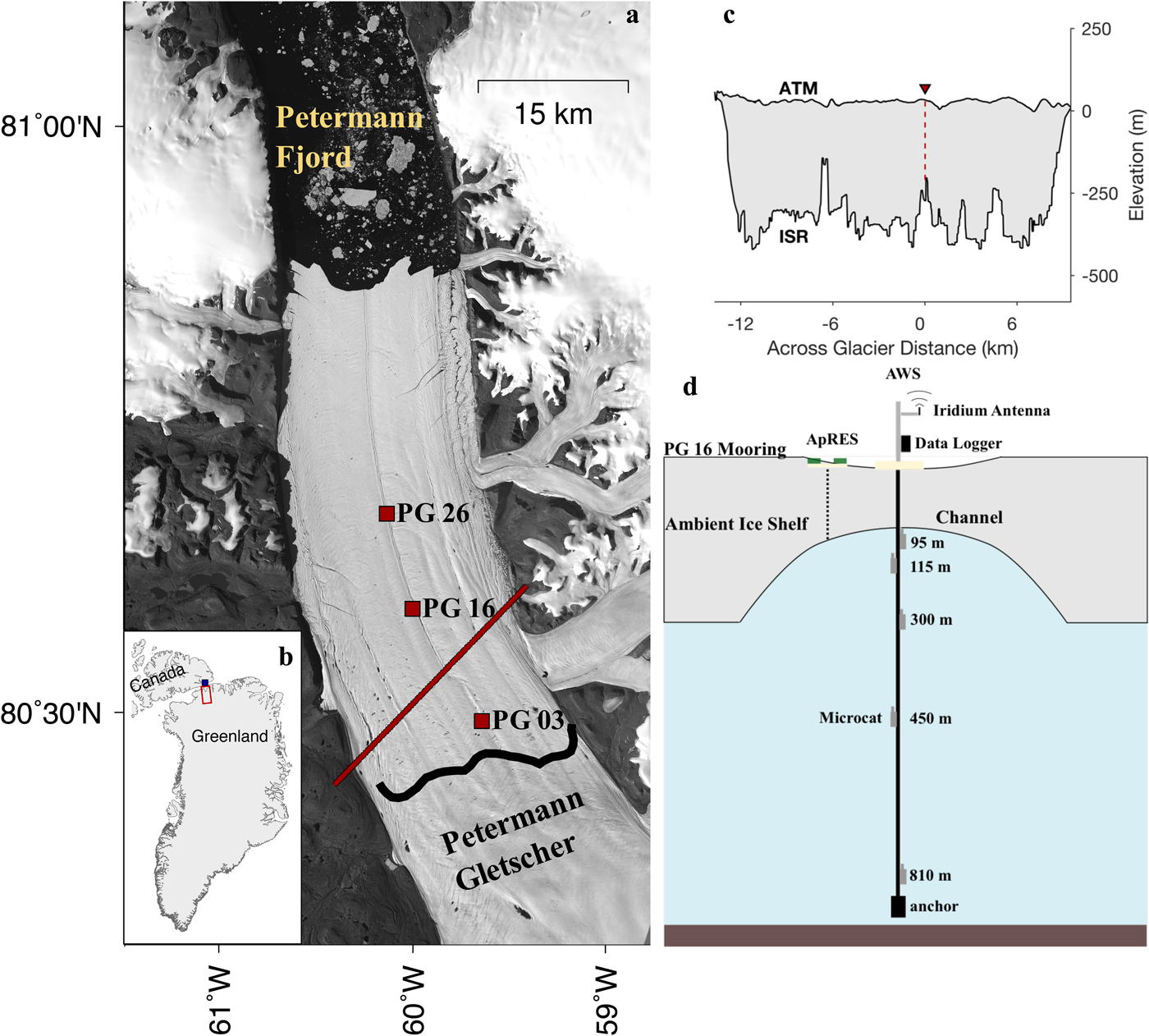
Fig. 1. (a) Landsat 8 image from 12 August 2015 displaying Petermann Gletscher in NW Greenland. Burgundy squares indicate the locations of the 2015 drill sites, burgundy line shows the Operation Icebridge flight line from 31 March 2014, and black line represents the glacier's grounding line. (b) The larger geographic region: red box outlines the region shown in (a) and blue square provides the location of the Discovery Harbor tide gauge. (c) PGIS elevation profile from the Operation Icebridge flight with a red arrow and dashed line marking the central sub-ice-shelf channel. Basal elevations come from the multichannel ice-sounding radar (ISR) carried during the flight and surface elevation come from the Airborne Topographic Mapper (ATM) (Krabill and others, Reference Krabill2002). (d) Schematic of the PG 16 mooring.
2. METHODS
2.1. Data acquisition
In August 2015, we used a hot water drill to make three holes through PGIS. These holes were positioned along the axis of the central sub-ice-shelf channel of PGIS at 3 km (PG 03: 80.58°N, 59.07°W), 16 km (PG 16: 80.66°N, 60.50°W) and 26 km (PG 26: 80.74°N, 60.78°W) seaward of the grounding line (Fig. 1a). The ice at these sites was 380, 100 and 100 m thick, respectively. Drill sites PG 16 and PG 26 were positioned at the apex of the channel where the ice was thinnest, but drill site PG 03 lay on the flank of the channel in thicker ice. After drilling each hole, we collected Conductivity-Temperature-Depth (CTD) profiles then deployed oceanographic moorings beneath the ice shelf. This study focuses on data from PG 16, but also includes select observations from PG 03 and PG 26.
The PG 16 mooring (Fig. 1d) comprised five Sea-Bird SBE-37 SM Microcat sensors beneath the ice shelf and an automatic weather station (AWS) on the ice shelf surface. Here we utilize air temperatures from a Vaisala HMP155 sensor on the AWS. A data logger with an Iridium modem transmitted the oceanographic and atmospheric data in real time. An Autonomous phase-sensitive Radio-Echo Sounder (ApRES) ~10 m away from the PG 16 mooring measured local ice shelf thickness, which was converted to time-varying basal melt rates using the methodology described by Nicholls and others (Reference Nicholls2015). The specific application to our site is summarized below (Section 2.3). Partial failures of the PG 16 mooring system led to gaps in the atmospheric and oceanographic datasets during the periods of 11 February 2016 to 28 August 2016, and 20 December 2016 to 22 February 2017. The ApRES system stored data locally and relayed a subset via Iridium datalink. Therefore, it did not experience these data gaps; however, data messages stopped on 2 May 2017.
The PG 03 and PG 26 oceanographic moorings each contained two Sea-Bird SBE-37 SM Microcat sensors, one in the upper ocean and one at depth. Here we discuss data from the upper ocean sensors, which only reported for a short time after their deployment. The PG 26 sensor failed on 17 September 2015 after recording for 1 month, then the PG 03 sensor followed on 28 November 2015 after recording for 3.5 months. All Microcat sensors were cross-calibrated with a shipboard SBE 911+ CTD profiler prior to deployment in 2015, following the methodology of Kanzow and others (Reference Kanzow, Send, Zenk, Chave and Rhein2006). Table 1 lists the associated sensor uncertainties along with other related information.
Table 1. Hydrographic instruments

Tidal data come from a Paroscientific pressure sensor moored 125 km northwest of PGIS in Discovery Harbor, Canada (Münchow and Melling, Reference Münchow and Melling2008) (Fig. 1b). The instrument recorded bottom pressure from 2003 to 2012. We use a harmonic least squares fit with 38 tidal constituents to make tidal predictions for PGIS. Münchow and others (Reference Münchow, Padman, Washam and Nicholls2016) compared these predictions with tidal oscillations from a differential GPS at PG 26 and found that the two sites experienced minimal differences in tidal amplitude and phase. Tides are predominantly semidiurnal (see Münchow and others (Reference Münchow, Padman, Washam and Nicholls2016) Fig. 4), with a pronounced fortnightly cycle in tidal range from 0.5–1 m at neap tides to ~2 m at spring tides.
2.2. Converting GoPro footage into a light backscatter profile
After drilling through the ice shelf at each site, we took a gravity core to collect sediment, and also to determine the seafloor depth. This was done by recording the amount of line payed out when the sediment corer impacted the seafloor. We mounted a GoPro HERO4 video camera to the Kevlar tether line, just above the sediment corer. The GoPro recorded video at 30 frames per second, with a 1080p resolution and a fixed ISO of 1600. A water and pressure-resistant housing protected the GoPro while it collected footage of the sub-ice-shelf water column at each site. An LED mounted beside this housing illuminated the dark ocean. Regions of the water column with higher densities of suspended sediment reflected more of this light back toward the video camera than regions with less sediment. The recorded light level averaged across each frame provided an estimate of the light backscatter from suspended sediment in the water column. At PG 16 we recorded the time elapsed while tracking the amount of line out during sediment core collection. The amount of line out was recorded every minute, with a constant descent speed assumed between readings. This allowed us to convert the light level output file into a depth profile of light backscatter by suspended sediment in the water column. Although we did not record the time elapsed during sediment collection at the other two locations, video footage from these sites provided qualitative information about suspended sediment in the sub-ice-shelf water column (Fig. 2).
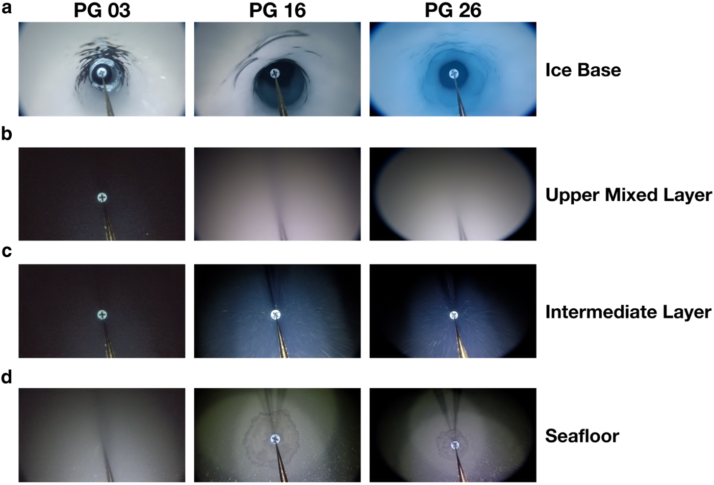
Fig. 2. Images of the sub-ice-shelf water column from GoPro HERO4 videos taken while collecting sediment cores at each study site.
2.3. ApRES melt rates
The ApRES is a frequency-modulated continuous wave (FMCW) radar that was configured to collect a burst of 20, one-second long samples every hour. Each sample consists of a FMCW ‘chirp’ covering a frequency range from 200 to 400 MHz. Each set of 20 chirps was averaged and then processed to create a complex depth profile of phase and amplitude using the steps described by Brennan and others (Reference Brennan, Lok, Nicholls and Corr2014). Monitoring the phase of the radar return from the base of the ice allows the changing range between the antennas and the ice base to be observed throughout the year with a precision determined by the signal to noise ratio of the basal echo. In the case of a shallow, cold ice column such as at PG 16, the signal to noise ratio for the basal echo is high, resulting in a precision better than 1 mm.
For the ice shelf of Petermann Gletscher we expect the range between the ApRES antennas and the ice base to change as a result of ice strain, ablation at the upper surface and melting at the ice shelf base. The presence of internal reflections from within the ice column allows the effect of upper surface melt and ice strain to be removed, and the changing basal melt rate to be quantified. Temporal changes in the basal geometry and radio wave velocity through the ice, due to changes in ice properties, could affect the accuracy of the basal melt rate measurements. However, the stability of the shapes of the basal echo and the internal reflections in our data indicate that these possible effects can be ignored.
The vertical strain rate was found to be approximately constant throughout the year, and contributed a thickening of 3.3 ± 0.3 m a−1. The uncertainty in the vertical strain rate measurement was found by calculating the uncertainty in a weighted least squares fit of a straight line to the vertical profile of internal-layer displacements. The weightings were estimated from the vertical profile of signal to noise ratio, which was itself calculated from the variance of the signal across the 20 chirps. The surface ablation rate was found by measuring the uniform upward motion of internal layers, and offsetting by their depth-dependent downward motion due to the strain thickening. Surface ablation was negligible over the record except during the 2016 summer months, when it contributed to a thinning of 1.4 ± 0.2 m. The estimated uncertainty in the surface ablation rate, therefore, had contributions from the uncertainty both in the strain rate and in the uniform upward motion of the layers. Overall, the uncertainties in the basal melt rate were dominated during the non-summer months by uncertainty in the vertical strain rate (± 0.3 m a−1), and during the summer by uncertainty in the surface ablation rate (± 0.5 m a−1).
2.4. Water mass partition
We employ a three-point water mass partition to calculate the concentrations of glacial meltwater (GMW) produced by ocean-forced basal melting and SR in the sub-ice-shelf water column. This partition assumes that water properties in the sub-ice-shelf water column of PGIS can be described as a mixture of three different water masses: GMW, SR and Atlantic Water (AW). Beaird and others (Reference Beaird, Straneo and Jenkins2015) showed that most glacially fed fjord systems around Greenland contain more than three water masses. A potential fourth water mass to be considered is the cold and fresh polar water that occupies the upper water column of the uncovered section of Petermann Fjord (Straneo and others, Reference Straneo2012). Johnson and others (Reference Johnson, Münchow, Falkner and Melling2011) identified the presence of this water mass beneath the eastern shear margin of PGIS in 2002. However, during a 2015 research cruise to Petermann Gletscher the presence of polar water was confined to the upper 50 m of the uncovered Petermann Fjord water column, well above the 200 m average ice base depth at the PGIS terminus at that time (Heuzé and others, Reference Heuzé, Wåhlin, Johnson and Münchow2017). A strong pycnocline separated this upper layer from the underlying water column, with density increasing by ~2.5 kg m−3 between 50 and 100 m depth. We, therefore, assume that the concurrent 2015 sub-ice-shelf CTD profiles were unaffected by polar water. We also discount any significant influence of polar water on our upper ocean time series data. We show below that during the initial 3 months of time series data a seaward flow prevailed near the ice base that resembled a buoyant, meltwater-rich plume (Section 3.4). In addition, heavy sea-ice cover near PGIS throughout most of the year significantly reduces the likelihood of wind and buoyancy-forced mixed layer deepening permitting advection of polar water beneath the ice shelf to our sites (≥24 km from the terminus).
Thus, we follow the methodology of Jenkins (Reference Jenkins1999) and use Conservative Temperature (Θ) and Absolute Salinity (S A) characteristics to compute the mixture of GMW and SR in the sub-ice-shelf water column:


The Conservative Temperature and Absolute Salinity characteristics of GMW consider the latent heat loss that results from a phase change from solid to liquid freshwater (Conservative Temperature and Absolute Salinity will hence be referred to as temperature and salinity for brevity). This gives GMW an effective temperature of − 92.5°C at 0 g kg−1, considering an ice temperature of − 20°C (Equation (2) of Jenkins (Reference Jenkins1999)). The temperature-salinity (T-S) characteristics of SR, on the other hand, simply represent freshwater at a pressure-depressed freezing point of − 0.38°C and 0 g kg−1, consistent with the PGIS grounding line depth of 500 m (Rignot and Steffen, Reference Rignot and Steffen2008). At the time of the 2015 sub-ice-shelf CTD profiles the T-S characteristics of AW were 0.27°C and 34.93 g kg−1. However, Washam and others (Reference Washam, Münchow and Nicholls2018) showed that the T-S properties of the AW beneath PGIS have trended toward warmer and saltier over the past decade. We observe a continuation of this trend in our PG 16 time series at 450 m depth. From 23 August 2015 to 26 October 2017, Θ and S A increased at this depth from 0.27°C and 34.93 g kg−1 to 0.35°C and 34.97 g kg−1. When computing the water mass partition for our time series data we incorporate the Θ and S A at this depth smoothed with a 10-day running median filter. Note that this range in AW properties only imparts a change in GMW and SR concentrations of 0.1 and 0.05%, respectively.
3. RESULTS
3.1. Seasonal variability in basal melt at PG 16
The basal melt rate data from the PG 16 ApRES point to a strong seasonal cycle in melting (Fig. 3). For much of the year, the 2-day filtered basal melt rate ranged from 0 to 10 m a−1, with a mean of 2 m a−1 (Fig. 3c). Over this time period, air temperatures persisted below freezing and the ocean adjacent to PGIS was largely covered with sea ice (Figs 3a, b). Basal melting then increased dramatically with the onset of the 2016 summer season when air temperatures exceeded freezing for 2.5 months and the sea-ice cover retreated considerably. During this time period, the basal melt rates at PG 16 reached a maximum of 80 m a−1, with a mean of 23 m a−1 (Fig. 3). Basal melting at PG 16 promptly declined after air temperatures dropped below freezing and the 2016 summer season ended. Over the following 7 months melt rates remained below 5 m a−1. Seaice cover gradually increased over this time, but appeared more variable than the previous year. Failure of the PG 16 ApRES Iridium datalink on 2 May 2017 prevented acquisition of basal melt measurements during the 2017 summer when air temperatures exceeded 0°C and the sea ice retreated once again (Fig. 3).
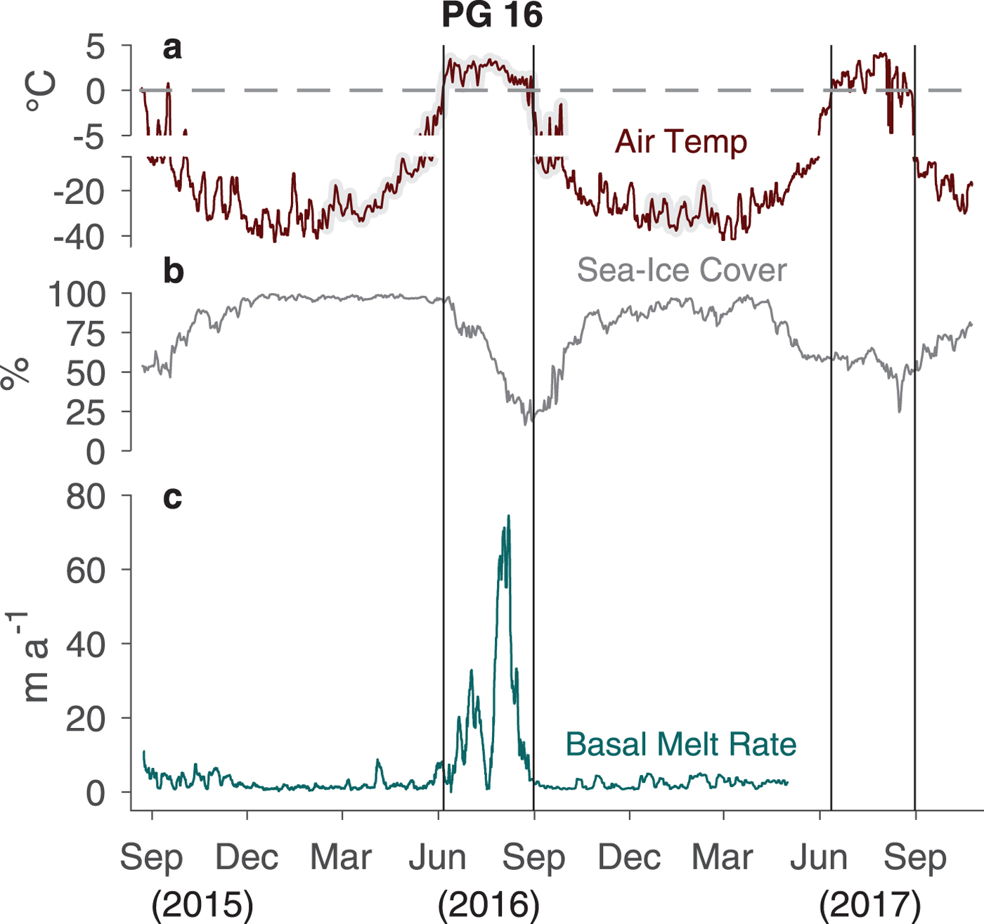
Fig. 3. (a) AWS air temperature time series from PG 16 smoothed with a 2-day running median filter. (b) Daily SSM/I sea ice cover near PGIS (81°N–82°N, 60°W–67°W) from NSIDC archives at 25 km resolution (Steffen and Schweiger, Reference Steffen and Schweiger1991). (c) Basal melt rate time series from PG 16 smoothed with a 2-day running median filter. Grey-shaded air temperatures come from updated output of the 1 km resolution downscaled RACMO2.3 model (Noël and others, Reference Noël2016) for PGIS. Black vertical lines indicate the 2016 and 2017 summer seasons when air temperatures exceeded 0°C (grey dashed line).
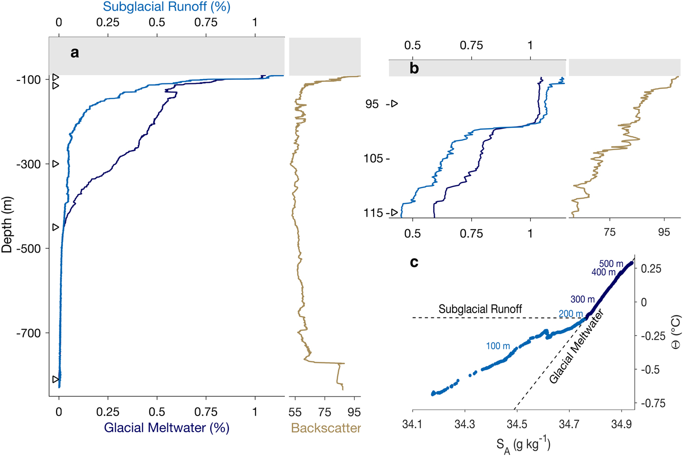
Fig. 4. (a) Depth profile of subglacial runoff and glacial meltwater concentration beneath PGIS at PG 16, with the grey-filled box indicating ice shelf thickness and the black triangles marking moored instrument depths. Gold line depicts backscatter from a coincident GoPro HERO4 video, which serves as a proxy for light attenuation by suspended sediment. (b) Same as (a), but focused on the upper 20 m of the water column. (c) Temperature versus salinity diagram of the PG 16 CTD profile with depth markers and Glacial Meltwater and Subglacial Runoff mixing lines, as described by Gade (Reference Gade1979) and Straneo and others (Reference Straneo2012), respectively.
Over the 619-day ApRES data record (22 August 2015 to2 May 2017) the ice shelf at PG 16 experienced a total thinning of 4.4 ± 0.5 m, after considering basal melting, surface melting and opposing thickening from vertical ice strain. All of this thinning occurred over the 80-day summer season when heightened basal melt rates along with surface melt rates outpaced background strain thickening rates. Remote-sensing imagery from the 2016 summer showed extensive surface melting on Petermann Gletscher from 25 km upstream of the grounding line to the ice shelf terminus (Macdonald and others, Reference Macdonald, Banwell and MacAyeal2018). Surface melting began in mid June and persisted until late August, consistent with the period of above-freezing air temperatures and elevated basal melt rates at PG 16. Recent modeling suggests that this heightened summer basal melting results from a larger flux of SR across the grounding line, as a result of surface meltwater that has drained to the ice base (Cai and others, Reference Cai, Rignot, Menemenlis and Nakayama2017). However, reduced sea-ice cover during the 2016 summer may also have raised basal melt rates through advection of warmer water underneath the ice shelf from its terminus (Shroyer and others, Reference Shroyer, Padman, Samelson, Münchow and Stearns2017). To determine what drives variability in the basal melt rate at PG 16, we investigate the sub-ice-shelf ocean data.
3.2. Sub-ice-shelf water masses
A CTD profile collected in August 2015 provided a snapshot of the full sub-ice-shelf water column at PG 16. Washam and others (Reference Washam, Münchow and Nicholls2018) analyzed the T-S characteristics of this profile and identified the presence of AW, GMW from basal melting and SR. Here we use these T-S characteristics to calculate the concentration of GMW and SR beneath the ice shelf at PG 16. We also use light backscatter data from a GoPro HERO4 video as a proxy for suspended sediment concentration in the sub-ice-shelf water column (Section 2.2).
At the time of the PG 16 CTD profile, the concentrations of both SR and GMW in the sub-ice-shelf water column were greatest near the ice base (Fig. 4a). Within the upper mixed layer, SR and GMW registered at maximum concentrations of 1.2 and 1.1%, respectively (Fig. 4b). We also observed considerable suspended sediment in this region of the water column which produced high levels of backscatter in the GoPro video (Fig. 4b). Below this mixed layer, the concentration of suspended sediment and SR in the water column decreased quickly (Fig. 4a). The relationship between SR and suspended sediment indicates that this freshwater entered the ocean at the grounding line rather than directly via moulins or rifts through the ice shelf itself. The concentration of GMW declined gradually with depth, approaching zero near 500 m. In T-S space the slope exhibited by the PG 16 profile between the ice base and 230 m was ~ 1°C g−1 kg−1, consistent with the mixture of AW with both SR and GMW (Fig. 4c). Between 230 and 500 m depth this slope became steeper and adhered to the 2.5°C g−1 kg−1 change that results from ice melting, i.e. input of GMW, into AW (Gade, Reference Gade1979). Below ~500 m we observed the presence of undiluted AW.
CTD profiles were also collected at PG 03 and PG 26 in August 2015 (Fig. 5). The PG 26 profile exhibited a comparable structure to the PG 16 profile, with a high concentration of SR (2.5%) and GMW (1%) in the upper mixed layer (Figs 5b, c). Similar to PG 16, the SR concentration at PG 26 decreased quickly with depth and the GMW concentration declined gradually down to near-zero at ~500 m depth. While we did not acquire a backscatter profile at this site, a still frame from the GoPro video identified the SR tracer of copious suspended sediment in the upper mixed layer (Fig. 2b). The PG 03 profile lacked the T-S and suspended sediment signatures of SR in the upper water column (Figs 2b, 5a). We suspect that this is because PG 03 lay on the flank of the channel instead of at its apex where the SR was identified at the other sites.
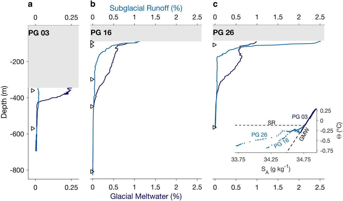
Fig. 5. Depth profiles of subglacial runoff and glacial meltwater concentration at (a) PG 03, (b) PG 16, and (c) PG 26, with the grey-filled box indicating ice shelf thickness and the black triangles marking moored instrument depths. The inset of (c) provides the T-S diagram for these profiles with GMW and SR mixing lines, as described by Gade (Reference Gade1979) and Straneo and others (Reference Straneo2012), respectively.
3.3. Ice/ocean interactions at PG 16
The basal melt rate at any location beneath an ice shelf depends on the turbulent flux of heat into the ice base from the underlying ocean. This heat flux is largely a function of the ocean temperature relative to freezing and the under-ice current speed, which dictates the efficiency of how ocean heat turbulently mixes into contact with the ice base (Jenkins, Reference Jenkins1991). Partial mooring system failure prevented the acquisition of oceanographic measurements at PG 16 during the 2016 summer when high basal melt rates (Fig. 3c) indicated a large flux of ocean heat into the ice base. However, the first 6 months of ocean data from this site (23 August 2015 to 11 February 2016) covered the transition from late summer 2015 into winter 2015/16. During this period, 2-day time-averaged basal melt rates were low (Fig. 3c), but unfiltered melt rates (Fig. 6a) occasionally exceeded 15 m a−1. These data may, therefore, provide insight into how the ocean interacts with the ice shelf during periods of heightened basal melting.
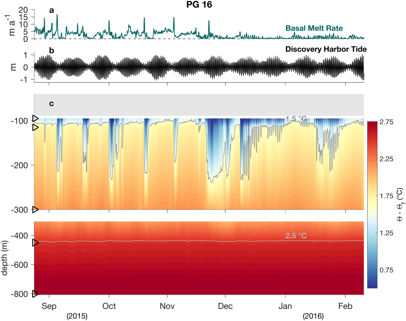
Fig. 6. (a) Unfiltered PG 16 basal melt rates from 23 August 2015 to 11 February 2016 with grey dashed 0 m yr−1 line. (b) Discovery Harbor tidal oscillations over this time computed with a harmonic fit, which was used to advance 2002–13 data in time. (c) Pseudo colored under-ice ocean temperatures above freezing considering pressure and salinity effects. Grey-filled box represents the ice shelf thickness, black triangles indicate instrument depths, and contours show temperatures of 1.5 and 2.5°C above freezing.
We observe a highly variable ice-ocean environment within the central channel of PGIS over this time period (Fig. 6). Sub-ice-shelf ocean temperatures range from 0.12 to 1.25°C above the pressure-dependent freezing point within 5 m of the ice base in the upper mixed layer, with substantial variability throughout the upper water column (Fig. 6c). Unfiltered basal melt rates vary from minimum values near 0 m a−1 to maxima of 18 m a−1 (Fig. 6a). Between 23 August and 22 November 2015, we observe peaks in basal melting at PG 16 that commonly occur before or during neap tides (Fig. 6b). During these peaks, melt rates exceed 10 m a−1 for a ~10 hour interval. Afterward, upper ocean temperatures plunge by ~ 1°C, suggesting the arrival of considerable meltwater into the water column. Cold ocean conditions and near-zero melt rates typically persist until tidal amplitudes increase and then higher ocean temperatures return. This pattern ends with a final peak in melting on 22 November. The timing of this peak differs from others as it occurs when tidal amplitudes increase rather than decrease. The cold ocean conditions that follow persist through spring tide until the end of the subsequent neap tide. After this event basal melt rates remain below 5 m a−1 and follow a different pattern, fluctuating primarily at semidiurnal and diurnal tidal frequencies over the next 2.5 months. The upper ocean likewise varies primarily at tidal frequencies after 8 December which suggests a regime shift in the coupled ice shelf-ocean system.
A water mass analysis of the uppermost ocean sensor data reveals a connection between the concentration of SR and GMW in the upper mixed layer at PG 16, the local basal melt rate and the tide over this time (Fig. 7). The cold ocean pulses that occurred during neap tides in the first half of the record (August--December) contained higher concentrations of both SR and GMW (Figs 7b–d). During these meltwater pulses, the SR and GMW concentration in the upper mixed layer rose considerably over background values to reach maximum concentrations of 2.8 and 1.9%, respectively. We interpret these signals as advective pulses of GMW that result from the periodic discharge of SR across the PGIS grounding line. The high concentration of SR in the meltwater pulses supports this interpretation. Peaks in local basal melting preceded these ocean meltwater pulses (Fig. 7a). We attribute this increased melting to stronger under-ice current speeds induced by the discharge of buoyant SR at the grounding line. When the resultant ocean meltwater pulse arrived at PG 16, local melt rates declined due to the low temperatures now present in the ocean adjacent to the ice base.
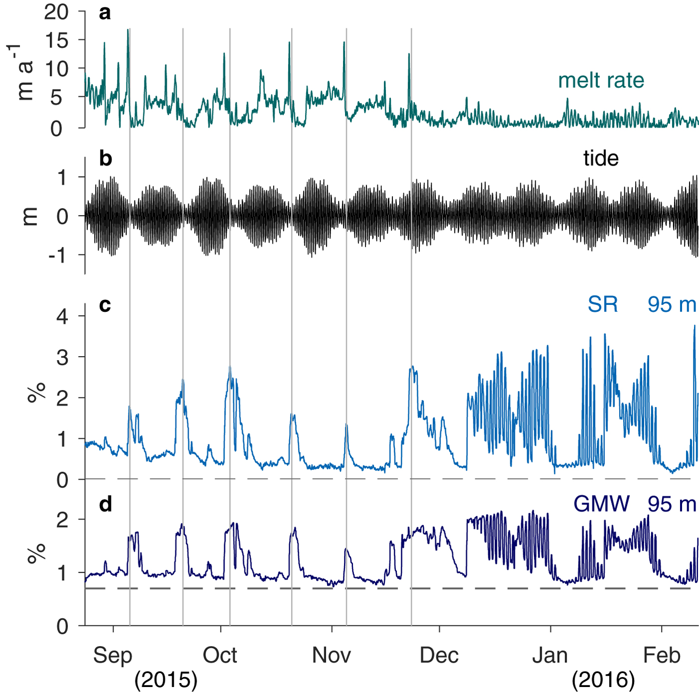
Fig. 7. (a) Unfiltered PG 16 basal melt rates from 23 August 2015 to 11 February 2016. (b) Computed Discovery Harbor tidal oscillations over this time. (c) PG 16 upper mixed layer subglacial runoff (SR) concentration at 95 m depth / within 5 m of ice base; grey dashed line denotes 0% SR concentration. (d) PG 16 upper mixed layer glacial meltwater (GMW) concentration at the same depth.
The background SR concentration in the upper mixed layer decreased from 0.9% in August to ~0.2% in December (Fig. 7c). Background GMW values also decreased somewhat over this period from 1 to 0.7% (Fig. 7d). This decline in SR and GMW concentration at PG 16 implies a weakening of the buoyancy-driven flow over this time. Large vertical gradients in SR and GMW concentration near the base of the upper mixed layer (Figs 4 and 5) indicate that this apparent decline might also result from a shoaling of the mixed layer past our sensor. These processes are coupled. We expect buoyancy-driven flow to be the largest component of under-ice currents. Models indicate that tidal currents under PGIS are very weak (Padman and others, Reference Padman, Siegfried and Fricker2018) and that, within 20 km of the grounding line, currents forced by atmospheric variability and ocean instabilities seaward of the ice shelf terminus are also weak (Shroyer and others, Reference Shroyer, Padman, Samelson, Münchow and Stearns2017). Higher currents drive higher turbulent stresses at the ice base and lead to a thicker mixed layer; therefore, as buoyancy-driven flow weakens, we expect a thinner mixed layer and a further reduction in background SR and GMW concentrations measured at a fixed distance from the ice base.
After the final SR-induced basal melt rate peak and ocean meltwater pulse, we observe a regime shift to a tide-dominated ice shelf-ocean system. During this second half of the record (December--February), the basal melt rate and the upper mixed layer SR and GMW concentrations at PG 16 exhibit large variability at the fundamental tidal frequencies of ~1 and ~2 cycles per day. Concentrations and melt rates appear largest when tidal amplitudes are high and we expect tidal currents to be strongest. However, the comparatively low melt rates over this period indicate that these tidally driven currents are weaker than the buoyancy-driven currents from before, consistent with modeling results (Padman and others, Reference Padman, Siegfried and Fricker2018). Hence, we expect a thinner upper mixed layer and the large fluctuations in SR and GMW concentration at 95 m depth to result from the mixed layer base oscillating past the sensor. Additionally, we attribute the high SR and GMW concentrations observed during this time to the advection of these water masses to PG 16 during the prior meltwater pulse. A period of weak buoyancy-driven currents then allowed cold and fresh water to remain at PG 16, and for tidal currents to dominate the ice/ocean interactions.
3.4. Propagation of glacial meltwater pulses beneath PGIS
In addition to the PG 16 mooring, ocean sensors were also deployed at PG 03 and PG 26, within 15 and 20 m of the ice base, respectively (Figs 5a, c). These instruments recorded for only a short period of time; however, during this time their data also contained pulses of GMW (Fig. 8b) that were induced by the periodic discharge of SR at the grounding line. We investigate the evolution of meltwater pulses beneath PGIS over this short-time period when upper ocean sensors recorded at all three mooring sites. Note that here we incorporate data from the PG 16 sensor moored at 115 m depth (within 25 m of ice base), because it resided at a similar distance from the ice base as the upper sensors at PG 03 and PG 26.
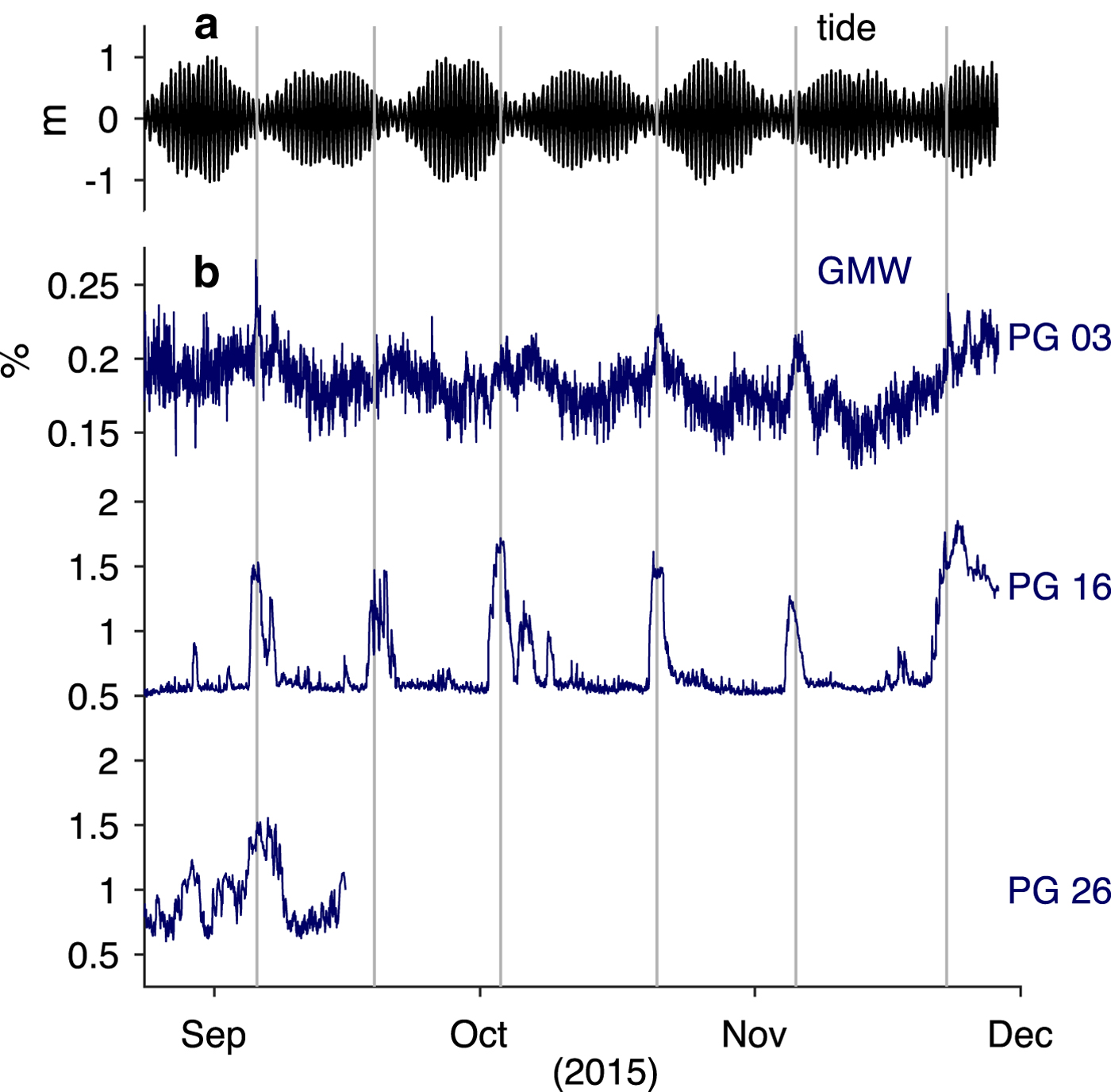
Fig. 8. (a) Computed Discovery Harbor tidal oscillations. (b) Upper ocean glacial meltwater (GMW) concentration at PG 03, PG 16 and PG 26. Instrument depth/distance from ice base: PG 03 (360 m/15 m), PG 16 (115 m/25 m), PG 26 (110 m/20 m).
From late August through November 2015, meltwater pulses occurred at PG 03 and PG 16 during neap tides (Figs 8a, b). At PG 03 they manifested as 0.05% spikes in GMW above background values (0.2%). As previously discussed, the pulses appeared much clearer at PG 16, with GMW concentration rising from 0.5% to ~1.5%. The lone meltwater pulse sampled at PG 26 in early September 2015 contained a similar concentration to PG 16, although it was broader in time.
The PG 03 upper ocean sensor was moored beneath the flank of the sub-ice-shelf channel; therefore, observed GMW concentrations during meltwater pulses at this site may not have represented the full signal nearby at the channel apex. Nevertheless, the considerable enrichment of GMW between PG 03 and PG 16 in these pulses implies that substantial basal melting occurred between these two locations, which is consistent with melt rate estimates from remote sensing (Rignot and Steffen, Reference Rignot and Steffen2008; Münchow and others, Reference Münchow, Padman and Fricker2014; Wilson and others, Reference Wilson, Straneo, Heimbach and Cenedese2017). This is not the case between PG 16 and PG 26, where GMW concentrations appear similar during the one observed meltwater pulse.
The buoyant meltwater plume model of Jenkins (Reference Jenkins2011) shows that plume speeds should depend on the sine of the ice base angle. Since the base of PGIS sloped upward between PG 03 and PG 16, then flattened out between PG 16 and PG 26, we expect a faster plume between PG 03 and PG 16 than between PG 16 and PG 26.
We estimate the advection speed of meltwater pulses by computing phase lags between sites. Due to the short record length of the PG 26 sensor and therefore poor frequency resolution, we first compute time domain phase-lagged cross correlations between data. This yields an average R2 correlation and lag over all frequencies. Our cross correlations show that 45% of GMW variance at PG 16 correlates with that at PG 03, with PG 16 signals lagging by 12 hours. The PG 26 GMW variability likewise correlates with 51% of that at PG 16, with PG 26 signals lagging by 62 hours. From these lags, we estimate signal propagation speeds of 0.30 m s−1 between PG 03 and PG 16 (13.12 km apart) and 0.05 m s−1 between PG 16 and PG 26 (9.82 km apart). The differing signal speeds qualitatively agree with an upward sloping and then flattened ice base between sites. However, the specific frequency associated with these phase lag-derived signal speeds cannot be extracted from this time domain approach.
The longer concurrent data records at PG 03 and PG 16 allow us to resolve correlations and phase lags at a set of discrete frequencies that are multiples of 1/T, where T is the effective record length (53 days). This record length represents half of the full concurrent record length (106 days), which was split in two and ensemble averaged to reduce uncertainty. At the principal meltwater pulse frequency of 0.07 cycles per day, 85% of the GMW variance at PG 16 correlates with that at PG 03 (Fig. 9). This highly correlated oscillation occurs first at PG 03 with a 19° phase lead relative to that at PG 16. The 19° phase difference of a co-oscillation at the 14-day timescale represents a time lag of 16 hours, corresponding to a velocity of 0.23 m s−1. We interpret this velocity as the advective speed of a buoyant meltwater plume moving from PG 03 to PG 16 that was triggered every 2 weeks during this time period by processes related to discharge of SR at the grounding line and vertical mixing.
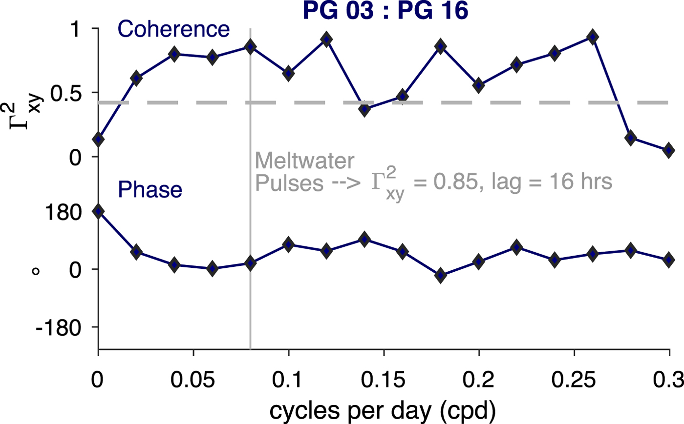
Fig. 9. Results from partial coherence test for Glacial Meltwater (GMW) concentration between PG 03 (360 m depth) and PG 16 (115 m depth). Upper panel: Fraction of PG 16 GMW variance that is coherent with PG 03 variance for specific frequencies between 0 and 0.3 cycles per day. Lower panel: Phase offset associated with these coherence values. Vertical grey line marks the approximate frequency for meltwater pulses. Grey dashed line indicates the 95% significance level for coherence values based on a Chi-squared distribution considering 4 degrees of freedom.
3.5. Seasonal variability in subglacial runoff
The full time series from the uppermost ocean sensor at PG 16 displays a seasonal signal in upper ocean SR and GMW mixture overlaid on a downward trend in these concentrations (Figs 10a–d). We interpret this downward trend as a consequence of the increasing distance between the sensor and the ice base due to basal melting (Fig. 10b). As the ice base retreated, the sensor resolved the upper mixed layer with progressively lower accuracy. Nevertheless, the data clearly indicate a lagged relationship between upper ocean SR and GMW concentration and above-freezing air temperatures (Figs 10a, c, d). During the transition from late summer to winter in 2015/16 and 2016/17, air temperatures declined from > 0°C to − 40°C, but the concentration of SR and GMW in the upper ocean at PG 16 remained high. These concentrations then decreased considerably in February to June period of 2017, which covered the remainder of the winter season. With the onset of summer 2017, air temperatures rose above freezing and the mixture of SR and GMW in the upper ocean again increased, although not substantially until 1 month after the arrival of above-freezing air temperatures. With respect to the SR concentration, we propose that this 1-month lag indicates the time taken for atmospherically generated surface meltwater on the grounded portion of the glacier to reach the grounding line, then discharge into the ocean and arrive at PG 16. However, the modest rise in SR concentration prior to this large signal implies that some surface meltwater drains quickly to the ice base, then discharges across the grounding line into the ocean.
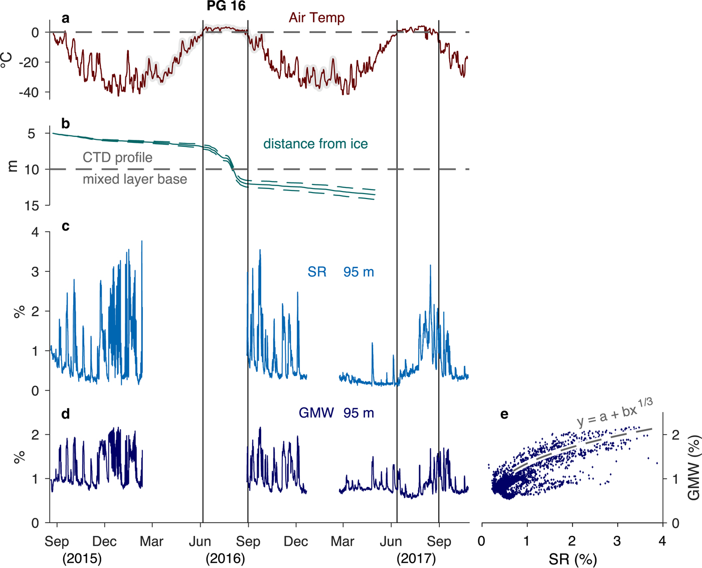
Fig. 10. (a) AWS air temperature time series from PG 16 smoothed with a 2-day running median filter; grey-shaded data come from 1 km downscaled RACMO2.3 model output and black vertical lines denote 2016 and 2017 summer seasons when air temperatures exceeded 0°C (grey dashed line). (b) Upper sensor distance from ice base due to basal melting, with green dashed lines representing uncertainty from ice shelf vertical strain (± 0.3 m a−1) and surface melting (± 0.5 m a−1). Grey dashed line indicates mixed layer base from PG 16 CTD profile (Fig. 4). (c) Full subglacial runoff (SR) and (d) glacial meltwater (GMW) concentration time series from PG 16 ocean sensor at 95 m depth. (e) GMW versus SR with least square regressional fit: GMW(%) = a + b*SR(%)1/3 for data that exceed +1 STD of the median GMW concentration. Uncertainty associated with this regression at a 95% confidence limit: a (0.01% ± 0.36%), b (1.38 ± 0.31), RMS residuals (0.34%). The regression analysis follows methodology described by Fofonoff and Bryden (Reference Fofonoff and Bryden1975) and considers 156 Degrees of Freedom, resulting from the greater of the decorrelation timescales for GMW and SR concentrations.
Over the 2 year time series, the concentration of GMW in the upper ocean at PG 16 varied concurrently with the SR concentration. Pulses of GMW, induced by the discharge of SR at the grounding line, occurred throughout the data record, although their frequency and amplitude decreased noticeably during the 2016/17 winter season. As shown above, during the first 3 months of data these pulses were preceded by peaks in the local basal melt rate (Fig. 7). This suggests that the discharge of buoyant SR at the grounding line strengthened under-ice currents at PG 16. The enrichment of GMW between PG 03 and PG 16 in these pulses further indicates that this was not a localized process (Fig. 8), but that strengthened buoyant flow drove substantial basal melting along the base of the central channel of PGIS between these sites. The buoyant plume model of Jenkins (Reference Jenkins2011) showed that modeled basal melt rates along a section of an ice shelf increased at a one-third power of the SR flux across the grounding line. We apply a one-third power least square regression (GMW(%) = a + b * SR(%)1/3) to data from the meltwater pulses over the full record, and find RMS residuals of 0.34% (Fig. 10e). The relationship between increased SR and GMW concentration at PG 16 agrees with the model results. Therefore, the rise in SR and GMW mixture during the 2017 summer suggests a similar seasonal rise in basal melt rates, as observed in 2016 (Fig. 3). The relatively rapid decline in SR and GMW concentrations following the end of the 2017 summer season differs from the gradual decrease observed during the previous 2 years. We interpret this decline to be caused by a further retreat of the ice base away from our sensor, due to heightened basal melting occurring once again during the 2017 summer months (Fig. 10b). This further supports our assertion that the discharge of SR across the grounding line directly influences the rate at which PGIS melts in its central channel.
4. DISCUSSION
Our in-situ oceanographic and glaciological measurements provide insight into how PGIS interacts with the underlying ocean in one of its large, longitudinal channels. Upper water column T-S properties display the influence of SR at two of the three study sites: PG 16 and PG 26. At both of these sites, this SR carries a tracer of suspended sediment. The third study site, PG 03, lacked the T-S and suspended sediment signatures of SR in the upper water column. We suspect that this is because PG 03 lay on the flank of the channel instead of at its apex where we identified the SR at the other sites. The absence of SR at PG 03 indicates the spatially and temporally focused nature of this outflow, and that correct sensor positioning becomes more difficult near the grounding line. The connection between suspended sediment and SR at PG 16 and PG 26 agrees with observations from tidewater glaciers around Greenland where surface expressions of buoyant, sediment-laden upwelling plumes highlight the presence of SR during summer (Bartholomaus and others, Reference Bartholomaus2016; Mankoff and others, Reference Mankoff2016; Jackson and others, Reference Jackson2017).
Basal melt rate and upper ocean property time series from PG 16 show the direct influence of SR on basal melting. For much of the year when air temperatures remain below freezing, basal melt rates are low. However, intermittent peaks in basal melting during this time correspond to GMW-rich ocean pulses that depend on the associated mixture of SR, consistent with results from under-ice plume modeling that show SR enhances melting (Jenkins, Reference Jenkins2011).
We also observed meltwater-rich pulses at PG 03 and PG 26. Phase lags from temporal and spectral analyses reveal that signals propagated seaward during neap tides at speeds that varied with the slope of the ice base. Estimated signal speeds were higher between PG 03 and PG 16 (0.23 m s−1), where the ice base rose by 255 m over a distance of 13120 m (a slope of 1.1°), than between PG 16 and PG 26 (0.05 m s−1) where the ice base registered at the same depth. The concentration of GMW in these pulses also increased considerably between PG 03 and PG 16, but not between PG 16 and PG 26 (in the one meltwater pulse sampled at PG 26). This behavior is consistent with that of a buoyant meltwater plume which evolves as a function of the sine of the ice base angle and the plume's temperature above freezing (Equation (14) of Jenkins (Reference Jenkins2011)). Following this reasoning, we attribute the higher propagation speeds between PG 03 and PG 16 to the 1.1° ice base angle and higher ocean temperatures, and the lower speeds between PG 16 and PG 26 to the negligible ice base angle and lower temperatures that resulted from the addition of GMW. Alternatively, these pulses could result from internal wave activity. The phase speed of a non-dispersive internal wave considering an upper layer thickness between 15 and 25 m (sensor distances from ice base), a reference density of 1027 kg m−3, and a 1 kg m−3 density difference across an interface would be 0.40–0.50 m s−1. This phase speed is computed using linear long wave theory where internal wavelengths are assumed to be much greater than the upper layer thickness and wave amplitudes are assumed to be smaller than the upper layer thickness. Nonlinear wave effects may also apply to this scenario (Nash and Moum, Reference Nash and Moum2005).
The slower propagation speed of the signals, apparent dependency upon the ice base angle and GMW enrichment between sites lead us to attribute them to the periodic strengthening of a buoyant meltwater plume. We attribute this strengthening to the intermittent discharge of SR across the grounding line. The timing of these discharge events could relate to tidally-driven migration of the PGIS grounding line (Hogg and others, Reference Hogg, Shepherd, Gourmelen and Engdahl2016), which affects pressure gradients in the upstream subglacial hydrological system (Walker and others, Reference Walker2013).
The presence of SR in the water column well after the end of the surface melt season points to a persistent subglacial hydrological system that likely contains remnant summer surface meltwater (Schoof and others, Reference Schoof, Rada, Wilson, Flowers and Haseloff2014). At PG 16 the concentration of SR in the upper ocean diminished with time following the end of the 2016 summer season until it reached a minimum during the months of February to June in 2017. With the onset of the 2017 summer surface melt season, air temperatures exceeded freezing for ~1 month and then the concentration of SR increased substantially. We interpret this lag as the time required for surface meltwater produced over the grounded Petermann Gletscher catchment to arrive at the grounding line, then discharge into the ocean and arrive at our site. The elevated SR mixture at PG 16 over the next 1.5 months indicates that surface meltwater continued to augment the flux of SR across the PGIS grounding line during this time. While we lacked basal melt rates for the 2017 summer, during the 2016 summer we did observe a dramatic increase in basal melt rates at PG 16 that resulted from this increased flux of SR. The elevated basal melt rates during this season outpaced the 3.3 ± 0.3 m a−1 background strain thickening rate and, along with 1.4 ± 0.2 m of surface melt, caused the ice shelf to thin by 4.4 ± 0.5 m at this location.
Previous observational studies focused on the role that ocean warming played on the rapid ice shelf loss experienced by Greenland glaciers Jakobshavn Isbrae (Holland and others, Reference Holland, Thomas, De Young, Ribergaard and Lyberth2008) and Zachariae Isstrom (Mouginot and others, Reference Mouginot2015). For PGIS, realistic ocean simulations suggest that basal melt rates along the thinner outer portion of the ice shelf respond to seasonal changes in sea ice conditions and upper water column heat content of the surrounding ocean (Shroyer and others, Reference Shroyer, Padman, Samelson, Münchow and Stearns2017). However, this seasonality does not extend to the inner portion of PGIS where the ice draft is greater. Furthermore, this ocean variability accounts for only a 20% variability in the integrated melt rate, which is much smaller than the ~1000% increase in the mean basal melt rate that we observe at PG 16 from winter to summer. Instead, our results are more consistent with those from an idealized 2-D model of PGIS that explored melt rate sensitivity to variations in the flux of SR (Cai and others, Reference Cai, Rignot, Menemenlis and Nakayama2017). Our observations confirm that increased SR during summer from surface meltwater draining to the glacier bed greatly enhances basal melt rates in one of the PGIS channels, which leads to thinning in this already thin region of the ice shelf. Focused, channelized thinning can form transverse fractures (Dow and others, Reference Dow2018) which spread and contribute to large calving events that force ice shelf retreat. Our results, therefore, indicate that the length and intensity of future summer surface melt seasons will play a major role in the stability of PGIS.
ACKNOWLEDGMENTS
Both the National Science Foundation (NSF) and National Aeronautics and Space Administration (NASA) supported this work. We are grateful to crew and staff aboard the Swedish Ice Breaker Oden in 2015 who made this work possible by providing helicopter support for field operations on the glacier. Alan Mix of Oregon State University generously shared time and resources in the field in 2015. Paul Anker and Mike Brian of the British Antarctic Survey provided critical support for hot water drilling and glacier traveling. The PG 16 atmospheric and oceanographic mooring was designed and built by David Huntley at the University of Delaware and funded by NASA grant NNX15AL77G. AM was supported by a subcontract from Jet Propulsion Laboratory in 2015 and NSF grant 1604076 in 2016. LP was supported by NSF grant 1708424 and NASA grant NNX17AG63G. We thank Emily Shroyer, who generously shared her model output, as well as Tore Hattermann and one anonymous reviewer for their thoughtful comments during the revision process.
AUTHOR CONTRIBUTIONS
PW wrote the text, produced the figures and processed air temperature, ocean property, Landsat 8 and Operation Icebridge data, under of supervision of AM, KWN and LP. AM, KWN and LP contributed to writing the paper and advising on figures. PW, AM and KWN collected air temperature and ocean property data. AM designed, tested and facilitated the acquisition, distribution and initial processing of data from the PG 16 mooring. KWN collected ApRES data and processed them to acquire basal melt rates. PW and KWN collected and processed the GoPro HERO4 light-level data to produce the backscatter profile in Fig. 4.


 Open access