
Abstract
History matters when individual prior conditions contain important information about the fate of individuals. We present a general framework for demographic models which incorporates the effects of history on population dynamics. The framework incorporates prior condition into the i-state variable and includes an algorithm for constructing the population projection matrix from information on current state dynamics as a function of prior condition. Three biologically motivated classes of prior condition are included: prior stages, linear functions of current and prior stages, and equivalence classes of prior stages. Taking advantage of the matrix formulation of the model, we show how to calculate sensitivity and elasticity of any demographic outcome. Prior condition effects are a source of inter-individual variation in vital rates, i.e., individual heterogeneity. As an example, we construct and analyze a second-order model of Lathyrus vernus, a long-lived herb. We present population growth rate, the stable population distribution, the reproductive value vector, and the elasticity of λ to changes in the second-order transition rates. We quantify the contribution of prior conditions to the total heterogeneity in the stable population of Lathyrus using the entropy of the stable distribution.
Introduction
Every demographic analysis requires a classification of individuals by age, size, developmental stage, physiological condition, or some other variable. These variables describe individual states (i-states) such that the fate of an individual depends only on its current state and the environment (Metz 1977; Caswell and John 1992; Metz and Diekmann 1986). This requires the state variable to capture all the aspects of the individual’s history that are relevant to its future fate (Caswell et al. 1972; Caswell 2001). The task of the population modeler is to find an i-state variable that successfully captures past history. This is not easy; apparently reasonable and frequently used choices of i-states may fail to capture all the relevant information about individual history.
Confronted with this problem, the modeler might choose a completely different i-state variable (as plant ecologists did when giving up age-classified demography in favor of size-classified models), or might add a dimension to the state space (as in extending stage-classified models to include both age and stage). Sometimes, however, it might be difficult or impossible to measure the relevant current characteristic, but a proxy for that characteristic might be found in some function of the prior condition of an individual. For example, resource storage can influence vital rates in plants but resource storage can be difficult to measure. However, reproduction in the prior year can be used as a proxy for resource storage in species where reproduction in one year may deplete resource storage and reduce fertility in the following year. If it is not possible to measure resource storage, one might therefore incorporate prior reproductive status into the state variable to improve the model.
A variety of prior conditions which affect vital rates have been found empirically. Reynolds and Burke (2011) found that chestnuts with fast early growth died younger than chestnuts with slow early growth. Warren et al. (2014) found that previous breeding success and current body condition may be among the most important determinants of breeding propensity in female lesser scaup. Rouan et al. (2009) found that choice of next breeding site is affected by both current and prior breeding site in Branta canadensis. These examples show that prior condition can be a source of individual variation in vital parameters, i.e., a source of heterogeneity. Some attempts have been made to include this source of heterogeneity into population models, see Pfister and Wang (2005), Ehrlén (2000), and Rouan et al. (2009), but a framework for incorporating general prior conditions into demographic models does not exist and will be presented in this paper.
When constructing a structured population model, the i-state variables are used to classify individuals into states in a population vector n(t) whose entries give the densities of each state. The population vector is projected forward by a population projection matrix A
The matrix A can be decomposed into a matrix U, containing transition probabilities for existing individuals, and a matrix F, describing the generation of new individuals by reproduction:
If prior conditions influence present dynamics, the vector n and the matrices U, F, and A must be modified to account for these influences. Our goal in this paper is to present a systematic method for constructing such models in which individuals are classified by current stage and (very generally defined) prior condition. Because we are considering effects of individual condition at just one prior time, we refer to these as second-order matrix population models. We will present the demographic analysis of such models at the level of the individual, the cohort, and the population, and show how to carry out sensitivity analyses of model results to changes in parameters. As an example, we develop a model and calculate the elasticity of the population growth rate of the herbaceous perennial plant Lathyrus vernus.
Terminology
Our discussion requires careful definitions of terms in order to clarify the way that historical effects are incorporated. We will say that the life cycle is described in terms of stages (e.g., size classes). The prior condition of an individual is some function of its stage at the prior time and its stage at the current time, and thus incorporates historical information. The combination of current stage and prior condition serves as the individual state variable for the analysis. We give an overview of the terminology used in this paper in Table 1.
The prior condition can be any arbitrary function of prior and current stage. Prior condition might be the stage at the prior time, it might be defined by membership in a set of stages at the prior time, or it might be defined as the difference between the current and the prior stages. Suppose for example that stages are defined by size, in the hope that a size classification would be a satisfactory i-state variable. It might turn out that historical effects require including size at the prior time in the i-state variable. Alternatively, the i-state might require information only on membership in a class of sizes (e.g., larger than average or smaller than average); we will refer to these classes of prior stages as equivalence classes. Or, the i-state might require information on the change in size between the previous time and the current time, and individuals might be classified by whether they have grown, shrunk, or remained in the same size class.
Models based on prior stage are described in section “Full prior stage dependence,” models based on general functions of prior and current stages are described in section “Prior condition models,” and models based on equivalence classes of prior stage are described in section “Equivalence classes of prior stages.” The matrices, vectors, and mathematical operations used in this paper are listed in Table 2.
Model construction
We will begin by constructing the model in which the prior condition is defined by full information on the prior stage, which we refer to as full prior stage dependence.
Full prior stage dependence
Creating a prior stage model requires transition and fertility rates to be measured for each possible prior stage. Since newborns do not have a well-defined prior stage in general, an extra prior stage must be added for newborns. If there are s current stages, we will label the prior condition of newborns as stage s + 1. Individuals are thus classified by their current stage 1,2,…,s and their prior stage 1,2,…,s + 1. The transition and fertility rates, conditional on prior stage, are given by the matrices U k and F k :
The entries of U k , denoted by \(u^{k}_{ij}\), are defined as
It is useful to think of the state of the population as described by a two-dimensional array N of size s × (s + 1)

where n i j is the number of individuals whose current stage is i and whose prior stage was j. Ehrlén (2000) suggested that this array could be updated by multiplication with a three-dimensional matrix. However, matrix multiplication can not be used directly to project such a two-dimensional array (this would require tensors). Instead, the two-dimensional array is transformed into a vector by stacking the columns on top of each other:
We use the tilde notation to denote vectors and matrices that relate to the prior condition model. The entries in the population vector \(\tilde {\mathbf {n}}\) are now ordered first by prior stage and then by current stage:

The vector \(\tilde {\mathbf {n}}\) is projected by a transition matrix \(\tilde {\mathbf {U}}\) and a fertility matrix \(\tilde {\mathbf {F}}\). The \(\tilde {\mathbf {U}}\) and \(\tilde {\mathbf {F}}\) matrices are constructed, respectively, from the set of matrices U k and F k . The transition matrix \(\tilde {\mathbf {U}}\) projects individuals into their next stage while keeping track of their prior stage. The matrix \(\tilde {\mathbf {U}}\) is written in terms of block matrices corresponding to the blocks in \(\tilde {\mathbf {n}}\) in Eq. 1. In Matlab notation, the transition matrix for a model with s = 2 is

where U k (:,i) refers to the i th column of the matrix U k and 0 is a column vector of size s × 1. To understand the structure of \(\tilde {\mathbf {U}}\), consider the (1,1) block in the upper left corner. This block projects individuals with prior stage 1 at t to prior stage 1 at t + 1. The only such individuals have current stage 1 at time t. They are projected by column 1 of U 1. All other columns of the (1,1) block of \(\tilde {\mathbf {U}}\) are zero. The other blocks of \(\tilde {\mathbf {U}}\) are filled similarly.
The blocks in the last row of \(\tilde {\mathbf {U}}\) are zero because transitions into the newborn stage are impossible; the matrix \(\tilde {\mathbf {F}}\) will fill up this row block. In general, for any number of stages s,
where e i has size s × 1 and E i j has size (s + 1) × (s + 1) and has a one in position (i,j) and zeros elsewhere.
The fertility matrix \(\tilde {\mathbf {F}}\) is constructed from the F i . Because individuals are always born into stage s + 1, the F i appear in the last row of blocks in \(\tilde {\mathbf {F}}\). For the case with s = 2, the fertility matrix is

In general, for any number of stages s,
where E (s+ 1)k has size (s + 1) × (s + 1) and has a one in position (s + 1, k) and zeros everywhere else.
Given a set of transition matrices U i and fertility matrices F i , Eqs. 11 and 13 define the second-order matrices \(\tilde {\mathbf {U}}\) and \(\tilde {\mathbf {F}}\), and the population projection matrix
These matrices are subject to all the usual demographic analyses, including population growth, population structure, and sensitivity analysis (see section “Case study” for an example).
Prior condition models
A more general second-order model structure allows transitions and fertility to depend on some function of current and prior stages. We consider the case where this function can be defined as a linear transformation of the full prior stage dependent model, where the population vector is written as \(\tilde {\mathbf {m}}\), defined by
for some matrix C. An example of such a prior condition is having previously grown, shrunk, or stayed the same size. The matrix C maps i-states defined by the combination of (current stage × prior stage) to i-states defined by the combination of (current stage × prior condition).
Suppose there are r distinct prior conditions. The state of the population is now given by a s × r array M

where m i j represents the number of individuals whose current stage is i and whose prior condition is j. As in Eq. 8, the population vector \(\tilde {\mathbf {m}}\) is
The key to the construction of the prior condition model is to derive C from the rule defining the prior condition. To do so, define a matrix ϕ
For example, if the r = 3 prior conditions are shrinking, stasis, and growth
Next, we define a set of matrices ϕ k(i,j), for k = 1,…,r, given by
Given the matrices ϕ k, the matrix C is given by
see Appendix A. To project the new population vector \(\tilde {\mathbf {m}}\), we replace the matrices \(\tilde {\mathbf {U}}\) and \(\tilde {\mathbf {F}}\) with new matrices \(\tilde {\mathbf {V}}\) and \(\tilde {\mathbf {G}}\), respectively, so that
The matrix \(\tilde {\mathbf {V}}\) describes transitions of extant individuals between the different i-states of the prior condition model and the matrix \(\tilde {\mathbf {G}}\) describes the production of new individuals in the prior condition model. Substituting (15) into both sides of Eq. 22 yields
Equation 23 is satisfied if \(\tilde {\mathbf {V}}\) and \(\tilde {\mathbf {G}}\) satisfy the following equations:
In general, the matrix C is not square and does not have an inverse. So we use the Moore-Penrose pseudo-inverse C ‡ (see Abadir and Magnus (2005)) to solve for \(\tilde {\mathbf {V}}\) and \(\tilde {\mathbf {G}}\):
If C is square and non-singular, the pseudo-inverse is the ordinary inverse:
If C is not square but has linearly independent rows (i.e., has full row rank),
If C has rows of zeroes (this happens if some combinations of current stage and prior conditions are impossible), then C will not have full rank. In this case, C ‡ is computed from the singular value decomposition, implemented in Matlab with the function pinv(C) and in R with the function Ginv(C). For example, in a size-classified model, it is impossible to be in the smallest size class and to have grown into it from a smaller size class. In such cases, C ‡ and thus also \(\tilde {\mathbf {V}}\) and \(\tilde {\mathbf {G}}\) have rows and columns of zeros corresponding to the impossible combinations.
Equations 26 and 27 define the prior condition matrices \(\tilde {\mathbf {V}}\) and \(\tilde {\mathbf {G}}\) and the population projection matrix
As in Eq. 14, the usual demographic results can be obtained from these matrices.
Equivalence classes of prior stages
Equivalence classes of prior stages are a special case of functions of current and prior stage. Equivalence classes are subsets of prior conditions that depend only on the prior stage. For example, individuals in a size-classified model might be categorized into two equivalence classes depending on whether they were previously above or below some threshold size.
The machinery described in the previous section, i.e., Eqs. 21, 26, and 27, can be used to write down the equivalence class model. However, there is an easier way to find the C matrix that transforms the full prior stage dependent population vector \(\tilde {\mathbf {n}}\) to the equivalence class population vector \(\tilde {\mathbf {m}}\). We transform the population matrix N in Eq. 1 into the equivalence class population matrix M in Eq. 1 by a matrix B;
The matrix B has size (s + 1) × r and its entries are
Applying the vec operator to Eq. 31 gives
where we have used the following result from Roth (1934) that vecA B C = (C T ⊗A)vecB. Equation 33 is a special case of Eq. 15 with
Since the rows of B ⊤ are orthogonal, the matrix B ⊤ and the matrix (B ⊤⊗I s ) both have full row rank and therefore C ‡ can be calculated from Eq. 29.
Sensitivity analysis
Sensitivity analysis provides the effect of changes in any parameter on any model outcome. In general, these computations require derivatives of scalar-, vector-, or matrix-valued functions with respect to scalar-, vector-, or matrix-valued arguments. Matrix calculus is a formalism which enables us to consistently calculate such derivates. For an introduction to matrix calculus, see Abadir and Magnus (2005); for details see Magnus and Neudecker (1988). Ecological applications of sensitivity analysis appear in Caswell (2007, 2009, 2012).
Consider some scalar or vector output of the model, ξ, which is computed from \(\tilde {\mathbf {U}}\) and \(\tilde {\mathbf {F}}\), or from \(\tilde {\mathbf {V}}\) and \(\tilde {\mathbf {G}}\). The matrices \(\tilde {\mathbf {U}}\), \(\tilde {\mathbf {F}}\), \(\tilde {\mathbf {V}}\), and \(\tilde {\mathbf {G}}\) are in turn computed from the matrices U i and F i . Suppose U i and F i depend on a p × 1 vector of parameters 𝜃, i.e., U i = U i [𝜃], then we use the chain rule to write
or
The first terms in Eqs. 35 and 36 capture effects through survival and transitions, and the second terms capture effects through fertility. The elasticities, or proportional sensitivities, are given by
The derivatives of \(\tilde {\mathbf {U}}\), \(\tilde {\mathbf {F}}\), \(\tilde {\mathbf {V}}\), and \(\tilde {\mathbf {G}}\) with respect to 𝜃 depend on how \(\tilde {\mathbf {U}}\) and \(\tilde {\mathbf {F}}\) depend on the U i and F i matrices. Differentiating (11), we obtain
Each term in the summation captures the effect of 𝜃 through one of the U i . The matrix \(\mathbf {Q}^{U}_{j}\) is given by
Similarly, differentiating (13) gives
where each term captures the effect of 𝜃 through one of the F i . The matrix \(\mathbf {Q}^{F}_{i}\) is given by
To calculate the derivatives of the prior condition matrices \(\tilde {\mathbf {V}}\) and \(\tilde {\mathbf {G}}\), we use the chain rule to write
Differentiating Eqs. 26 and 27, we obtain
Thus,
Equations 38 and 40 are substituted into Eq. 35. Equations 46 and 47 are substituted into Eq. 36. All that remains is to calculate the dependence of ξ on \(\tilde {\mathbf {U}}\) and \(\tilde {\mathbf {F}}\) (or \(\tilde {\mathbf {V}}\) and \(\tilde {\mathbf {G}}\)), and the dependence of U i and F i on the parameter 𝜃. These items are specific to the question under consideration, so we provide an example in the next section.
Case study
As an example, we apply the second-order formalism to a fully prior stage dependent model of a perennial plant. We will construct the model and calculate the population growth rate, the stable population vector, the reproductive value vector, and the elasticity of the population growth rate λ to proportional changes in the demographic rates.
Our analysis is based on a study by Ehrlén (2000) of Lathyrus vernus, a long-lived herb native to forest margins and woodlands in central and northern Europe and Siberia. Ehrlén classified individuals into seven stages: seed (SD), seedling (SL), very small (VS), small (SM), large vegetative (VL), flowering (FL), and dormant (DO). Ehrlén constructed two matrix models: a first-order model with no historical effects and a second-order model. We construct our second-order model from the transition and fertility rates calculated by Ehrlén (2000) (their Table 2).
We introduce a special prior stage for newborns; the second-order model therefore has a total of 7 × 8 = 56 states. We used Ehrlén (2000)’s demographic rates to construct a transition matrix U i and a fertility matrix F i for each of the eight prior stages. In Table 3, the transition matrix for individuals who were previously in stage SM is shown as an example. The first two columns of this matrix are zero because small plants can not go back to being seeds or seedlings. All eight transition and fertility matrices are in the Supplementary Material.
We constructed the projection matrix, \(\tilde {\mathbf {A}}\), from the U i and F i matrices using Eqs. 11 and 13. The resulting 56 × 56 matrices are available in the Supplementary Material. The population growth rate λ is given by the dominant eigenvalue of \(\tilde {\mathbf {A}}\),
This agrees with the value reported for the second-order model by Ehrlén (2000). Ehrlén also fitted a first-order model to the same data and found a value just above one (λ = 1.010). The stable population vector, \(\tilde {\mathbf {w}}\), and the reproductive value vector, \(\tilde {\mathbf {v}}\), which are displayed in Figs. 1 and 2, are the right and left eigenvectors of \(\tilde {\mathbf {A}}\), respectively. The entries of the stable population vector are denoted by \(\tilde {w}_{ij}\) for individuals with current stage i and prior stage j, analogously to the entries of the population vector \(\tilde {\mathbf {n}}\) in Eq. 1. The entries of the marginal stable current stage distribution, w c, are given by
and are shown in Fig. 1b. Similarly, the entries of the marginal stable prior stage distribution, w p, are given by
and are shown in Fig. 1c.

a Stable current stage × prior stage distribution. b Marginal current stage distribution. c Marginal prior stage distribution. Notation: seed (SD), seedling (SL), very small (VS), small (SM), vegetative large (VL), flowering (FL), dormant (DO), and newborn prior (NB)

a Reproductive value vector for each current stage × prior stage combination. b Marginal current stage reproductive value vector. c Marginal prior stage reproductive value vector. Notation: seed (SD), seedling (SL), very small (VS), small (SM), vegetative large (VL), flowering (FL), dormant (DO), and newborn prior (NB)
Individuals with the same current stage have different vital rates if they differ in prior stage and this heterogeneity due to prior stage affects the population growth rate λ. To quantify the relative effect of the different prior stage dependent transition matrices on the population growth rate, we calculate the elasticity of the population growth rate, λ, to changes in the U i matrices
Substituting λ for ξ in Eq. 37 yields
As shown in Caswell (2001),
where w i and v i are the right and left eigenvectors of U i , respectively, scaled so that
We sum the entries of Eq. 53 to get the elasticity of λ to a proportional change in all of the entries of U i . The results are shown in Fig. 3. We note that there are large differences among prior stages. Proportional changes in the demography of individuals with prior stages seed, seedling, or newborn have little effect on λ. Proportional changes in individuals who were small vegetative at the prior time have effects an order of magnitude larger.

The elasticity of λ to a proportional change in all of the U i
Discussion
When does history matter? Population models are based on i-state variables chosen by some mixture of biological intuition, tradition, practical limitations, and formal statistical analyses. Even after a careful choice of i-state, it may happen that individual prior conditions contain important information about the fate of individuals. In such cases, history matters, and the methods presented here solve the problem of how to incorporate information about it into matrix models.
Why stop at second-order effects, what about the effect of the prior condition at t − 2, t − 3, etc.? It is theoretically possible to extend the framework presented here to include dependence on higher-order effects. However, if the i-state variable is such that third- or even fourth-order historical effects are important, it might better to reconsider the choice of i-state variable instead of including ever increasing historical dependence.
Statistical tests for second-order effects in longitudinal data using log-linear models have been developed by Bishop et al. (1975) and Usher (1979). Time series of longitudinal data are needed to perform these tests as well as for the subsequent estimation of a prior condition dependent model. Capture–mark–recapture analyses for prior stage dependent models have been developed by Pradel (2005) and Cole et al. (2014).
Incorporating individual history requires a decision about what aspects of the prior condition are important. We have presented three biologically motivated cases: prior condition as the prior stage, prior condition as an arbitrary linear function of current and prior stages, and prior condition as an equivalence class of prior stages. In each case, the necessary information is a set of fertility and survival/transition matrices for each prior stage. The resulting models use block-structured matrices to project a vector of stages within prior conditions. These matrices can be used to calculate all the usual demographic outcomes. Because the matrices are carefully constructed from U i and F i , they can be subjected to sensitivity analysis. It is straightforward to calculate the sensitivity and elasticity of any model outcome to any parameters affecting the vital rates.
Prior condition effects are more than just a convenient tool in constructing i-states for population models. They are a biologically real source of inter-individual variation. The importance of individual variation in vital parameters to ecological processes has become increasingly evident in recent years (Bolnick et al. 2011; Valpine et al. 2014; Caswell 2014; Vindenes and Langangen 2015; Steiner and Tuljapurkar 2012; Cam et al. 2016). Ignoring individual variation in vital parameters, also referred to as individual heterogeneity, can have important consequences for the demographic outcomes and subsequent conclusions; see for example Vaupel et al. (1979), Rees et al. (2000), Fujiwara and Caswell (2001), Vindenes and Langangen (2015), and Cam et al. (2016). In his study of Lathyrus, Ehrlén (2000) found that including heterogeneity due to prior stage had only a small effect on λ, although it was sufficient to cause the population to decrease rather than increase.
How much heterogeneity is introduced by the prior condition effects in the Lathyrus example? Observations of individual plants can identify their current stage, but not their prior condition. The stable structure, \(\tilde {\mathbf {w}}\) (Fig. 1), shows the joint probability distribution over current and prior stages, and the amount of heterogeneity in the stable population can be calculated from the entropy of this distribution. The entropy of the joint current × prior stage distribution is
This measures the overall heterogeneity in the stable population structure. The heterogeneity in the marginal current stage distribution, w c [Eq. 49], is
This is the observable heterogeneity in current stage. The heterogeneity contributed by the unobservable prior stage, taking into account the relationship between current and prior stage, is
Khinchin (1957). Thus, in this example, the prior stage contributes about 35% of the total heterogeneity in the stable population.
In this paper, we have considered only linear models in constant environments. However, models could easily be constructed to include density effects, by making the U i and F i functions of density. Periodic or stochastic models could be constructed by making the U i and/or the F i appropriate functions of time. The analysis of the resulting models may pose interesting challenges and is an open research problem for population ecology.
References
Abadir KM, Magnus JR (2005) Matrix algebra, vol 1. Cambridge University Press
Bishop YMM, Fienberg SE, Holland PW (1975) Discrete multivariate analysis: theory and practice. MIT Press, Cambridge
Bolnick DI, Amarasekare P, Araújo M S, Bürger R, Levine JM, Novak M, Rudolf VH, Schreiber SJ, Urban MC, Vasseur DA (2011) Why intraspecific trait variation matters in community ecology. Trends Ecol Evol 26(4):183–192
Cam E, Aubry LM, Authier M (2016) The conundrum of heterogeneities in life history studies. Trends Ecol Evol 31(11):872– 886
Caswell H (2001) Matrix population models: construction, analysis, and interpretation, 2nd edn. MA, Sinauer Associates, Sunderland
Caswell H (2007) Sensitivity analysis of transient population dynamics. Ecol Lett 10(1):1–15
Caswell H (2009) Stage, age and individual stochasticity in demography. Oikos 118(12):1763–1782
Caswell H (2012) Matrix models and sensitivity analysis of populations classified by age and stage: a vec-permutation matrix approach. Theor Ecol 5(3):403–417
Caswell H (2014) A matrix approach to the statistics of longevity in heterogeneous frailty models. Demogr Res 31:553–592
Caswell H, John AM (1992) From the individual to the population in demographic models. In: Individual-based models and approaches in ecology. Springer, pp 36–61
Caswell H, Koenig HE, Resh J A, Ross QE (1972) Systems analysis and simulations in ecology. Vol II. In: Patten BC (ed) An introduction to systems science for ecologists. Academic Press, NY, pp 3–78
Cole DJ, Morgan BJ, McCrea RS, Pradel R, Gimenez O, Choquet R (2014) Does your species have memory? Analyzing capture–recapture data with memory models. Ecol Evol 4(11):2124–2133
Ehrlén J (2000) The dynamics of plant populations: does the history of individuals matter? Ecology 81 (6):1675–1684
Fujiwara M, Caswell H (2001) Demography of the endangered North Atlantic right whale. Nature 414:537–541
Khinchin A (1957) Mathematical foundations of information theory, vol 434. Dover Publications
Magnus JR, Neudecker H (1988) Matrix differential calculus with applications in statistics and econometrics. Wiley series in probability and mathematical statistics, Wiley
Metz HA (1977) State space models for animal behaviour. In: Annals of systems research. Springer, pp 65–109
Metz JAJ, Diekmann O (1986) The dynamics of physiologically structured populations Lecture notes in biomathematics. Springer-Verlag, Berlin
Pfister CA, Wang M (2005) Beyond size: matrix projection models for populations where size is an incomplete descriptor. Ecology 86(10):2673–2683
Pradel R (2005) Multievent: an extension of multistate capture–recapture models to uncertain states. Biometrics 61(2):442–447
Rees M, Mangel M, Turnbull L, Sheppard A, Briese D (2000) The ecological consequences of environmental heterogeneity. In: Hutchings MJ, John EA, Stewart AJA (eds) The effects of heterogeneity on dispersal and colonization in plants. Blackwell Science, Oxford, pp 237–265
Reynolds DL, Burke KL (2011) The effect of growth rate, age, and chestnut blight on american chestnut mortality. Castanea 76(2):129–139
Roth W (1934) On direct product matrices. Bull Am Math Soc 40:461–468
Rouan L, Choquet R, Pradel R (2009) A general framework for modeling memory in capture-recapture data. J Agricul Biol Environ Stat 14(3):338–355
Steiner UK, Tuljapurkar S (2012) Neutral theory for life histories and individual variability in fitness components. Proc Natl Acad Sci 109(12):4684–4689
Usher MB (1979) Markovian approaches to ecological succession. J Anim Ecol 413–426
Valpine P, Scranton K, Knape J, Ram K, Mills NJ (2014) The importance of individual developmental variation in stage-structured population models. Ecol Lett 17(8):1026–1038
Vaupel JW, Manton KG, Stallard E (1979) The impact of heterogeneity in individual frailty on the dynamics of mortality. Demography 16(3):439–454
Vindenes Y, Langangen Ø (2015) Individual heterogeneity in life histories and eco-evolutionary dynamics. Ecol Lett 18(5):417–432
Warren JM, Cutting KA, Takekawa JY, De La Cruz SE, Williams TD, Koons DN (2014) Previous success and current body condition determine breeding propensity in lesser scaup: evidence for the individual heterogeneity hypothesis. The Auk 131(3):287–297
Acknowledgements
We thank Gregory Roth for helpful discussions and Johan Ehrlén for providing the data for the Lathyrus case study.
Funding
This work was supported by European Research Council Advanced Grant 322989.
Author information
Authors and Affiliations
Corresponding author
Electronic supplementary material
Appendices
Appendix A: Derivation of the matrix C
In this appendix, we will derive the matrix C in Eq. 21, which transforms the fully prior stage dependent population vector, \(\tilde {\mathbf {n}}\), into the prior condition dependent population vector, \(\tilde {\mathbf {m}}\),
as in Eq. 15. Recall that we defined the matrix ϕ with elements
and we defined a set of indicator matrices ϕ k, for k = 1,…,r, given by
In Appendix B, we show a few examples of ϕ matrices. Recall furthermore the matrix

where n i j is the number of individuals whose current stage is i and whose prior stage was j, and the matrix

where m i j is the number of individuals whose current stage is i and whose prior condition was j. Finally, recall that the population vectors are given by
Using the above defined matrices ϕ k and N, the matrix M can be written as
The first term in the product is a matrix containing the densities of individuals in all entries of N that correspond to prior condition k, and zeros elsewhere. The second term in the product adds the densities across each row of the matrix ϕ k ∘N and puts these elements in the k th column of M. Taking the vec of both sides of this equation gives
where we have used vecA B C = (C T ⊗A)vecB (Roth 1934) and vec(A ∘B) = diag(vecA)vec(B). Comparison with Eq. 60 shows that
Appendix B: Examples of ϕ and C matrices
B.1 Examples of ϕ matrices
In this appendix, we show a few examples of the matrix ϕ.
-
(A)
When prior condition = prior stage, then
$$ \boldsymbol{\phi}(i,j)=j \text{ for all i.} $$(71)For example, when s = 3, ϕ is

-
(B)
When prior condition = equivalence classes of prior stages, then
$$ \boldsymbol{\phi}(i,j)=\text{function}(j) $$(74)For example, for s = 3 and for the case of the equivalence classes j = 1 and j > 1, we get
$$ \boldsymbol{\phi}(i,j) =\left\{ \begin{array}{ll} 1 & \text{for } j = 1 \\ 2 & \text{for } j = 2,3 \end{array}\right. $$(75)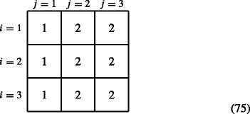
-
(C)
When prior condition = shrinkage, stasis, or growth, then
$$ \boldsymbol{\phi}(i,j) = \left\{ \begin{array}{lll} 1 & \text{for } i < j & \text{shrinkage} \\ 2 & \text{for } i=j & \text{stasis} \\ 3 & \text{for } i>j & \text{growth} \end{array}\right. $$(76)For example, for s = 3, ϕ is

-
(D)
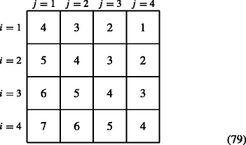
General more complicated growth conditions. For example, suppose the prior condition reflects the amount of growth, so that
$$ \boldsymbol{\phi}(i,j) = i-j +s. $$(78)For s = 4, this results in the following ϕ


B.2 An example C matrix
We consider the example in Eqs. 76 and 77 with three size classes and three growth classes corresponding to growth, shrinkage, and stasis. For simplicity, we consider a cohort model with no fertility and therefore no special prior condition for newborns. The matrices ϕ k are
Substituting these into Eq. 70, and letting the sum range from 1 to 3 only, gives the matrix C as

The transition matrix for the prior condition model, \(\tilde {\mathbf {V}}\), is given by Eq. 26 and requires the pseudo-inverse of the matrix C, which can be found using pinv(C) in Matlab or Ginv(C) in R. Substitution of the pseudo-inverse of C into Eq. 26 and a few lines of algebra result in

This matrix captures the complicated dependence of transitions on both current stage and prior condition. The placement of the weighted sums of transition probabilities from the U i matrices would be challenging without the methodology presented here.
Rights and permissions
Open Access This article is distributed under the terms of the Creative Commons Attribution 4.0 International License (http://creativecommons.org/licenses/by/4.0/), which permits unrestricted use, distribution, and reproduction in any medium, provided you give appropriate credit to the original author(s) and the source, provide a link to the Creative Commons license, and indicate if changes were made.
About this article

Cite this article
de Vries, C., Caswell, H. Demography when history matters: construction and analysis of second-order matrix population models. Theor Ecol 11, 129–140 (2018). https://doi.org/10.1007/s12080-017-0353-0
Received:
Accepted:
Published:
Issue Date:
DOI: https://doi.org/10.1007/s12080-017-0353-0