Abstract
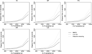
Recent studies have demonstrated theoretical attractiveness of a class of concave penalties in variable selection, including the smoothly clipped absolute deviation and minimax concave penalties. The computation of the concave penalized solutions in high-dimensional models, however, is a difficult task. We propose a majorization minimization by coordinate descent (MMCD) algorithm for computing the concave penalized solutions in generalized linear models. In contrast to the existing algorithms that use local quadratic or local linear approximation to the penalty function, the MMCD seeks to majorize the negative log-likelihood by a quadratic loss, but does not use any approximation to the penalty. This strategy makes it possible to avoid the computation of a scaling factor in each update of the solutions, which improves the efficiency of coordinate descent. Under certain regularity conditions, we establish theoretical convergence property of the MMCD. We implement this algorithm for a penalized logistic regression model using the SCAD and MCP penalties. Simulation studies and a data example demonstrate that the MMCD works sufficiently fast for the penalized logistic regression in high-dimensional settings where the number of covariates is much larger than the sample size.
References
Böhning, D., Lindsay, B.: Monotonicity of quadratic-approximation algorithms. Ann. Inst. Stat. Math. 40(4), 641–663 (1988)
Breheny, P., Huang, J.: Coordinate descent algorithms for nonconvex penalized regression, with application to biological feature selection. Ann. Appl. Stat. 5(1), 232–253 (2011)
Donoho, D.L., Johnstone, J.M.: Ideal spatial adaptation by wavelet shrinkage. Biometrika 81(3), 425–455 (1994)
Efron, B., Hastie, T., Johnstone, I., Tibshirani, R.: Least angle regression. Ann. Stat. 32(2), 407–451 (2004)
Fan, J., Li, R.: Variable selection via nonconcave penalized likelihood and its oracle properties. J. Am. Stat. Assoc. 96(456), 1348–13608 (2001)
Friedman, J., Hastie, T., Höfling, H., Tibshirani, R.: Pathwise coordinate optimization. Ann. Appl. Stat. 1(2), 302–332 (2007)
Friedman, J., Hastie, T., Tibshirani, R.: Regularization paths for generalized linear models via coordinate descent. J. Stat. Softw. 33(1), 1–22 (2010)
Hunter, D.R., Lange, K.: A tutorial on MM algorithms. Am. Stat. 58(1), 30–37 (2004)
Hunter, D.R., Li, R.: Variable selection using MM algorithms. Ann. Stat. 33(4), 1617–1642 (2005)
Jiang, D., Huang, J., Zhang, Y.: The cross-validated AUC for MCP-logistic regression with high-dimensional data. Stat. Methods Med. Res. (2011, accepted). doi:10.1177/0962280211428385
Lange, K.: Optimization. Springer, New York (2004)
Lange, K., Hunter, D., Yang, I.: Optimization transfer using surrogate objective functions (with discussion). J. Comput. Graph. Stat. 9(1), 1–59 (2000)
Mazumder, R., Friedman, J., Hastie, T.: SparseNet: coordinate descent with non-convex penalties. J. Am. Stat. Assoc. 106(495), 1125–1138 (2011)
Ortega, J.M., Rheinbold, W.C.: Iterative Solution of Nonlinear Equations in Several Variables. Academic Press, New York (1970)
Osborne, M.R., Presnell, B., Turlach, B.A.: A new approach to variable selection in least square problems. IMA J. Numer. Anal. 20(3), 389–403 (2000)
R Development Core Team: R: a language and environment for statistical computing. R Foundation for Statistical Computing, Vienna, Austria, ISBN 3-900051-07-0. http://www.R-project.org
Schifano, E.D., Strawderman, R.L., Wells, M.T.: Majorization-minimization algorithms for non-smoothly penalized objective functions. Electron. J. Stat. 4, 1258–1299 (2010)
Tibshirani, R.: Regression shrinkage and selection via the Lasso. J. R. Stat. Soc. Ser. B 58(1), 267–288 (1996)
Tseng, P.: Convergence of a block coordinate descent method for non-differentiable minimization. J. Optim. Theory Appl. 109(3), 475–494 (2001)
van de Vijver, M.J., He, Y.D., van’t Veer, L.J., et al.: A gene-expression signature as a predictor of survival in breast cancer. N. Engl. J. Med. 347(25), 1999–2009 (2002)
van’t Veer, L.J., Dai, H., van de Vijver, M.J., et al.: Gene expression profiling predicts clinical outcome of breast cancer. Nature 415(31), 530–536 (2002)
Warge, J.: Minimizing certain convex functions. SIAM J. Appl. Math. 11(3), 588–593 (1963)
Wu, T.T., Lange, K.: Coordinate descent algorithms for Lasso penalized regression. Ann. Appl. Stat. 2(1), 224–244 (2008)
Zhang, C.H.: Nearly unbiased variable selection under minimax concave penalty. Ann. Stat. 38(2), 894–942 (2010)
Zou, H., Li, R.: One-step sparse estimates in nonconcave penalized likelihood models. Ann. Stat. 36(4), 1509–1533 (2008)
Acknowledgements
The authors thank the reviewers and the associate editor for their helpful comments that led to considerable improvements of the paper. The research of Huang is supported in part by NIH grants R01CA120988, R01CA142774 and NSF grant DMS 1208225.
Author information
Authors and Affiliations
Corresponding author
Appendix
Appendix
In the appendix, we prove Theorem 1. The proof follows the basic idea of Mazumder et al. (2011). However, there are also some important differences. In particular, we need to take care of the intercept in Lemma 1 and Theorem 1, the quadratic approximation to the loss function and the coordinate-wise majorization in Theorem 1.
Lemma 1
Suppose the data (y,X) lies on a compact set and the following conditions hold:
-
1.
The loss function ℓ(β) is (total) differentiable w.r.t. β for any \(\boldsymbol{\beta} \in\mathbb{R}^{p+1}\).
-
2.
The penalty function ρ(t) is symmetric around 0 and is differentiable on t≥0; ρ′(|t|) is non-negative, continuous and uniformly bounded, where ρ′(|t|) is the derivative of ρ(|t|) w.r.t. |t|, and at t=0, it is the right-sided derivative.
-
3.
The sequence {β k} is bounded.
-
4.
For every convergent subsequence \(\{\boldsymbol{\beta}^{n_{k}}\} \subset\{\boldsymbol{\beta}^{n}\} \), the successive differences converge to zero: \(\boldsymbol{\beta}^{n_{k}} - \boldsymbol{\beta }^{n_{k}-1} \to0\).
Then if β ∞ is any limit point of the sequence {β k}, then β ∞ is a minimum for the function Q(β); i.e.
for any \(\boldsymbol{\delta}=(\delta_{0},\ldots,\delta_{p}) \in\mathbb {R}^{p+1}\).
Proof
For any β=(β 0,…,β p )T and \(\boldsymbol{\delta}_{j}=(0,\ldots,\delta_{j},\ldots,0) \in\mathbb {R}^{p+1}\), we have
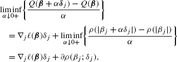
for j∈{1,…,p}, with
Assume \(\boldsymbol{\beta}^{n_{k}} \to\boldsymbol{\beta}^{\infty }=(\beta_{0}^{\infty},\ldots,\beta_{p}^{\infty})\), and by assumption 4, as k→∞

By (24) and (25), we have the results below for j∈{1,…,p}.
By the coordinate-wise minimum of jth coordinate j∈{1,…,p}, we have
Thus (26), (27) implies that for all j∈{1,…,p},

By (23), (28), for j∈{1,…,p}, we have
Following the above arguments, it is easy to see that for j=0
Hence for \(\boldsymbol{\delta}=(\delta_{0},\ldots,\delta_{p}) \in \mathbb{R}^{p+1}\), by the differentiability of ℓ(β), we have
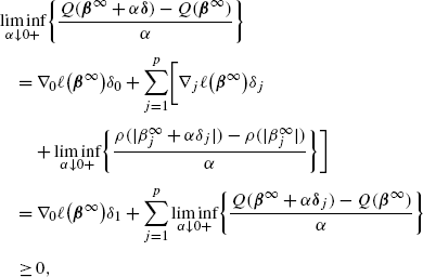
by (29), (30). This completes the proof. □
Proof of Theorem 1
To ease notation, write \(\chi_{\beta_{0},\ldots,\beta_{j-1},\beta _{j+1},\ldots,\beta_{p}}^{j}\equiv\chi(u)\) for Q(β) as a function of the jth coordinate with β l ,l≠j being fixed. We first deal with the j∈{1,…,p} coordinates, then the intercept (0th coordinate) in the following arguments.
For j∈{1,…,p}th coordinate, observe that
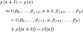
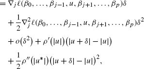
with |u ∗| being some number between |u+δ| and |u|. Notation ∇ j ℓ(β 0,…,β j−1,u,β j+1,…,β p ) and \(\nabla_{j}^{2}\ell(\beta_{0},\ldots,\beta_{j-1},u,\beta_{j+1},\ldots ,\beta_{p})\)denote the first and second derivative of the function ℓ w.r.t. the jth coordinate (assuming to be existed by condition (1)).
We re-write the RHS of (33) as follows:
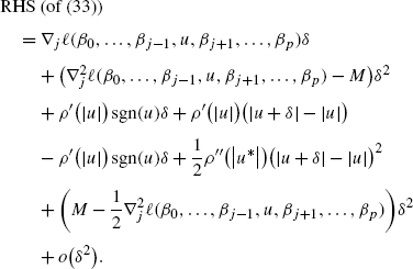
On the other hand, the solution of the jth coordinate (j∈{1,…,p}) is to minimize the following function,

By majorization, we bound \(\nabla_{j}^{2}\ell(\boldsymbol{\beta})\) by a constant M for standardized variables. So the actual function being minimized is
Since u minimizes (36), we have, for the jth (j∈{1,…,p}) coordinate,
Because χ(u) is minimized at u 0, by (37), we have
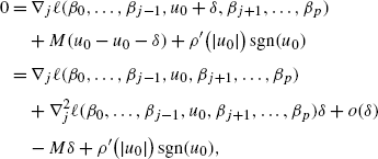
if u 0=0 then the above holds true for some value of \(\operatorname {sgn}(u_{0}) \in[-1,1]\).
Observe that ρ′(|x|)≥0, then

Therefore using (38), (39) in (34) at u 0, we have, for j∈{1,…,p},
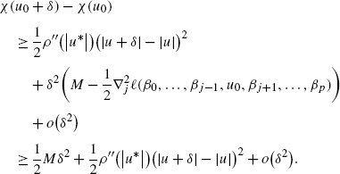
By the condition (b) of the MMCD algorithm inf t ρ″(|t|;λ,γ)>−M and (|u+δ|−|u|)2≤δ 2. Hence there exist \(\theta_{2}=\frac{1}{2}(M + \mbox{inf}_{x}\rho ^{\prime\prime}(|x|) + o(1)) >0\), such that for the jth coordinate, j∈{1,…,p},
Now consider β 0, observe that
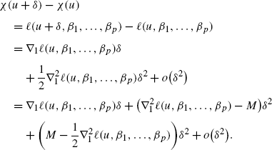
By similar arguments to (38), we have

Therefore, by (42), (43), for the first coordinate of β
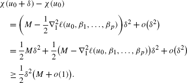
Hence there exists a \(\theta_{1}=\frac{1}{2} (M+ o(1)) >0\), such that for the first coordinate of β
Let θ=min(θ 1,θ 2), using (41), (45), we have for all the coordinates of β,
By (46) we have

where \(\boldsymbol{\beta}_{j}^{m-1}=(\beta_{1}^{m},\ldots,\beta _{j}^{m},\beta_{j+1}^{m-1},\ldots,\beta_{p}^{m-1})\). The (47) establishes the boundedness of the sequence {β m} for every m>1 since the starting point of \(\{ \boldsymbol{\beta}^{1}\} \in\mathbb{R}^{p+1}\).
Applying (47) over all the coordinates, we have for all m
Since the (decreasing) sequence Q(β m) converges, (48) shows that the sequence {β k} have a unique limit point. This completes the proof of the convergence of {β k}.
The assumption (3) and (4) in Lemma 1 holds by (48). Hence, the limit point of {β k} is a minimum of Q(β) by Lemma 1. This completes the proof of the theorem. □
Rights and permissions
About this article
Cite this article
Jiang, D., Huang, J. Majorization minimization by coordinate descent for concave penalized generalized linear models. Stat Comput 24, 871–883 (2014). https://doi.org/10.1007/s11222-013-9407-3
Received:
Accepted:
Published:
Issue Date:
DOI: https://doi.org/10.1007/s11222-013-9407-3


