

Abstract
Univentricular heart disease is the leading cause of death from any birth defect in the first year of life. Typically, patients have to undergo three open heart surgical procedures within the first few years of their lives to eventually directly connect the superior and inferior vena cavae to the left and right pulmonary arteries forming the total cavopulmonary connection (TCPC). The end result is a weak circulation where the single working ventricle pumps oxygenated blood to the body and de-oxygenated blood flows passively through the TCPC into the lungs. The fluid dynamics of the TCPC junction involve confined impinging jets resulting in a highly unstable flow, significant mechanical energy dissipation and undesirable pressure loss. Understanding and predicting such flows is important for improving the surgical procedure and for the design of mechanical cavopulmonary assist devices. In this study, dynamic mode decomposition (DMD) is used to analyze previously obtained stereoscopic particle imaging velocimetry (SPIV) data and large eddy simulation (LES) results for an idealized TCPC. Analysis of the DMD modes from the SPIV and LES serves to both highlight the unsteady vortical dynamics and the qualitative agreement between measurements and simulations.
Export citation and abstract BibTeX RIS
Communicated by H J Sung and P B Yoseph
1. Introduction
Children born with a single ventricle heart defect typically have to undergo a series of three open heart surgeries within the first few years of their life as part of a procedure known as Fontan palliation [1–3]. This staged process eventually results in a direct connection between the vena cavae (VC) and the pulmonary arteries forming what is known as the total cavopulmonary connection (TCPC) and a univentricular Fontan circulation. The TCPC geometrically consists of a four way confined intersection with blood flowing into the inferior vena cava (IVC) and superior vena cava (SVC), colliding at the TCPC junction and flowing passively into the Left and Right Pulmonary Arteries (LPA and RPA). The two confined impinging jets result in highly unstable and irregular flow as well as increased mechanical energy dissipation and pressure loss. Passively or actively reducing pressure losses is crucial in order to diminish the risk of heart failure by decreasing the load on the single working ventricle. Several research groups have focused on minimizing energy dissipation by preventing the two VC jets from colliding by introducing a caval offset [4] or by splitting one or both VCs [5, 6]. Several limitations are associated with each approach in terms of feasibility or lack of equal distribution of the hepatic flow between the two pulmonary arteries. In any case, a better understanding of these unstable flows to reduce these energy losses would help in improving the treatment techniques and the quality of life of the patients [7–10].
Delorme et al [11] carried out large eddy simulation (LES) of an idealized TCPC hemodynamic. They validated their simulations against measured stereoscopic particle imaging velocimetry (SPIV) data [12] and studied vortical structure dynamics. They observed bi-stable flow features in the pulmonary arteries related to the presence of one or two longitudinal vortical structures as well as the direction of their rotation alternating between clockwise and counterclockwise (see figure 6 in [11]). The one vs. two vortex feature was in agreement with experimental flow visualizations performed by Kerlo et al [12]. However, mean velocity profiles extracted downstream of the TCPC junction were not in agreement between the LES and SPIV data ([11], figure 5). In the simulations, because of the regular change of sign of the rotation inside the pulmonary arteries, the rotation of the flow was nullified when time averaged. This was clearly illustrated by the zero value of the out-of-plane (rotational) component of the mean velocity. On the other hand, mean velocity profiles from SPIV data showed that the flow rotated in one main direction, as only one main rotation of the flow was captured during the acquisition of the data. This showed limitation in the use of time averaged quantities to compare highly unstable phenomena.
In this study, dynamic mode decomposition (DMD) [13] is applied to the unstable flow of the TCPC junction. DMD is a method used to extract dynamic information from flow fields. These flow fields can come from numerical simulations or from time dependent experimental measurements. Using a finite number of data, DMD can then be used to gain a better understanding of the underlying physics captured, from a modal perspective. It can be used for many different applications that deal with flow instabilities [13–17]. Unlike the proper orthogonal decomposition method that extracts coherent spatial structures and ranks them using the energy content [18, 19], DMD extracts and ranks temporally coherent structures. In the next section, details on the implementation of the DMD algorithm are shown. The implementation is then validated using two benchmark cases. Finally DMD is applied to Fontan hemodynamics for both LES and SPIV data, to facilitate and improve the comparisons for this complicated flow. A summary concludes this paper.
2. Methods
2.1. DMD
The algorithm used follows the derivation of Schmid [13]. Let us assume a set of numerical or experimental data sampled at a constant frequency ( ). The data are then gathered in a sequence matrix;

where N is the number of samples and  is the ith flow field. We want to extract the Ritz values and vectors for this sequence:

We assume that a linear mapping A connects the flow field  to the subsequent flow field
  :
:

This linear assumption does not restrict the application of the DMD to linear flow fields. In the case of a nonlinear process, DMD can recover the dominant frequencies and associated modes when a sufficiently large number of snapshots is used [13, 14]. We can then write:

We are trying here to extract the characteristics of the dynamical process described by A. As the number of snapshots increase, it is safe to assume that the snapshots become linearly dependent. After a high enough number of snapshots, we have:

where r is the residual vector (a measure of the error induced by the linear independence assumption). We can then write:

where  is the
  unit vector and S is defined as:
The eigenvalues of S approximate some of the eigenvalues of A. A decomposition based on S is mathematically correct, but may be ill-conditioned, especially if noise is present in the data. A more stable formulation based on the singular value decomposition of the sequence matrix  is done instead:


Here, H denotes the conjugate transpose of a complex matrix, U and  are real or complex unitary matrix. It can be shown that U contains the proper orthogonal modes.
We can compute the eigenvalues and eigenvectors of  :
:

where  is the ith eigenvector associated with the eigenvalue
  . The DMD modes can then be computed using:

In order to know which modes are important, the temporal coherence of each mode can be computed as follow [13]:

and

In the following figures, the maximum temporal coherence is defined as:

where Y is the matrix containing the eigenvectors  . A summary of the procedure can be found in algorithm 1.
Algorithm 1. DMD of numerical or experimental data sets.
| 1. | Identify the region of interest |
| 2. | Extract 2D or 3D data sets with a constant time step 
|
| 3. | Build the data matrix  (equation 1) (equation 1) |
| 4. | Perform singular value decomposition to compute  (equation 9) (equation 9) |
| 5. | Compute the eigenvalues and eigenvectors of 
|
| 6. | Compute DMD modes (equation 11) |
| 7. | Rank the modes by computing the coherence |
2.2. Details of the LES simulations and stereoscopic particle image velocimetry (SPIV) measurements
In this study, the numerical simulations are performed using an in-house LES solver (WenoHemoTM ). This code is based on a 3D dimensionless incompressible formulation of the Navier-Stokes equations. The equations are integrated in time using a third order accurate backward difference formula method [20]. A fifth order accurate weighted essentially non oscillatory scheme is used to compute the convective terms [21]. The sub-grid stress tensor arising from the filtering of the equations is modeled using the constant coefficient Vreman sub-grid scale model [22]. In order to allow for simulations of complex geometries, the solver is coupled with a recent immersed boundary method [23]. More details can be found in [11] and [24].
Experimental data are obtained from Kerlo et al [12]. SPIV is applied at the junction of an idealized TCPC geometry connected to a mock circulation loop simulating single ventricle physiology, to obtain the three component of time dependent velocities in a plane centered in the pulmonary arteries. Details on the experimental conditions and procedures are given in [12].
3. Results
3.1. Validations
3.1.1. DMD of an analytical flow field:
In order to validate the implementation of the DMD algorithm, it is applied to a fabricated pattern similar to the one used by Seena et al [15]. The analytic flow q is the sum of four distinct modes, as shown below:

with

and
with

Table 1
shows the values of the coefficients  ,
,  ,
,  ,
,  and
and  for each of the modes.
  is constant in time.
  has a factor
  which means that its pattern does not grow or decay over time.
  has a factor
  that decreases as time passes, such that the particular pattern decays over time.
  on the other hand has a factor that induces a growth of the pattern as time passes. The analytic patterns q,
  ,
,  and
and  can be seen on figure 1.
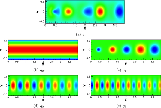
Figure 1. Analytic flow field q (t = 7.5 s). The four modes  ,
,  ,
,  and
and  are shown (b)–(e) as well as the sum q (a).
Download figure:
Standard image High-resolution imageTable 1. Values of the coefficients used in the analytic flow.
| n |

|

|

|

|

|
|---|---|---|---|---|---|
| 1 | 0.03 | 0.005 | 0.8 | 0.377 | 1 |
| 2 | 0.01 | 0.1 | 0.4 | 0.252 |

|
| 3 | 0.005 | 0.1 | 0.3 | 0.126 |

|
DMD analysis is performed using 200 snapshots with a constant time step of 0.05 s. A grid of 200 × 50 points is used. Figure 2(a) shows the extracted eigenvalues (real and imaginary parts). A typical circular pattern with the eigenvalues in complex conjugate pairs is observed. Figure 2(b) shows the same eigenvalues with frequencies ω plotted as a function of the growth rate σ. They are defined as:

and


Figure 2. Analytic flow field q: eigenvalues. The eigenvalues are represented in the complex plane (a) as well as in a logarithmic manner (b).
Download figure:
Standard image High-resolution imageIt is easily seen that most of the modes are stable (negative value of the growth rate). Four different modes are identified on figure 2(b) and corresponds to the four main eigenmodes extracted below. These eigenmodes are shown on figure 3: mode 1 corresponds to  . It is constant in time, which is why the frequency and growth rate are equal to zero. Mode 2 corresponds to
  : the frequency of the patterns are similar, and the value of
  is consistent with the absence of growth or decay of the pattern (
 ). Mode 3 shows a negative growth rate consistent with the decay of
  . Similarly, mode 4 shows a positive growth rate, consistent with the growth of the pattern 4. All these results are consistent with the fabricated pattern, and with the results reported by Seena et al [15].

Figure 3. Analytic flow field q: four selected DMD modes.
Download figure:
Standard image High-resolution image3.1.2. DMD of a 2D cylinder flow:
A 2D cylinder case is studied as the second validation case for the DMD algorithm. The approach of Chen et al [17] is followed. At a Reynolds number of 60, the dynamics of the flow can be decomposed into three phases: at the beginning of the simulation, the flow is stable and in equilibrium. The flow then transitions into a more unstable mode, to finally reach a limit cycle with vortex shedding in the wake of the cylinder. This last regime is studied using DMD here. Numerical simulations are performed using a 512 × 256 grid, and 30 snapshots are sampled using a constant time step of 0.4. Both the u and v-components of the velocity are used to build the data matrix  .
.
Figure 4(a) shows the Ritz values computed from the DMD. The eigenvalues are colored by coherence. Once again, a typical pattern close to the unit circle is observed. Three modes are highlighted, and are chosen because of their high temporal coherence. Figure 4(b) shows that all the eigenvalues are located on the left plane, indicating that all these modes are stable. Figure 4(c) shows the spectra. Very good agreement is observed between our simulation and the results reported by Chen et al. Figure 5 shows the z-vorticity with velocity vectors for the three selected eigenmodes. The first mode ( ) is shown in figure 5(a) and is representative of the mean flow with the typical shear layers developing from the top and bottom of the cylinder. Figure 5(b) shows mode 2 (
 ) with a symmetric pattern around the horizontal center-line. This mode corresponds to the convection of the large scales downstream of the cylinder. Mode 3 (
 ) shows an anti-symmetric profile which corresponds to the oscillations (shedding) of the vortices in the wake of the cylinder. These modes, as well as the complex velocity magnitudes (figures 5(c) and (e)) are in agreement with the results reported in [17].

Figure 4. 2D cylinder case: eigenvalues (a)–(b) and spectrum (c).
Download figure:
Standard image High-resolution image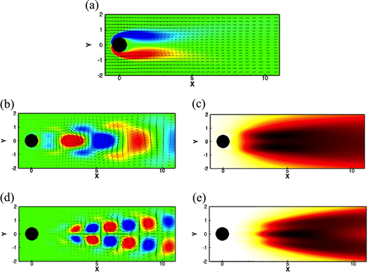
Figure 5. 2D cylinder case: three selected DMD modes.
Download figure:
Standard image High-resolution image3.2. DMD of Fontan hemodynamics in an idealized TCPC
In this study, two different geometries are considered and are shown in figure 6. The first one (figure 6(a)) is an idealized TCPC geometry without caval offset, similar to the one studied in [11] and [12]. Both LES and SPIV data are used to study the flow in this geometry. DMD is also applied to an idealized TCPC geometry with a caval offset of 0.5 diameter in the pulmonary arteries direction as shown in figure 6(b). For this second case, DMD is only applied to the numerical results as no experimental data are available. For both geometries, the red region in figure 6 represents the region where data are extracted and where DMD is applied. In both LES and SPIV, the flow rate imposed at each inlets is 2.2  and the viscosity of the fluid is 3.5 cP. The density of the fluid is 1060
  for the LES simulations and 1280
  for the SPIV experiments. The Reynolds number based on the inlet conditions is 700.
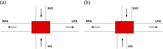
Figure 6. Schematic of the two TCPC geometries studied here (SVC: superior vena cava, IVC: inferior vena cava, LPA: left pulmonary artery, RPA: right pulmonary artery). The red region represents the domain where the DMD was performed.
Download figure:
Standard image High-resolution image3.2.1. DMD of an idealized TCPC without caval offset:
First, DMD is applied to the SPIV data. The focus is on the region centered at the junction of the TCPC and the data are sampled using a constant time step of 0.2 s (hundred snapshots). The domain size is 108 × 76 grid points. All three components of the velocity are used to build the data matrix  . Figure 7(a) shows the eigenvalues in a configuration around the unit circle. Four particular modes are highlighted: they are selected for their relatively high temporal coherence, as well as the absence of noise in the eigenmodes. These four eigenmodes can also be seen on figure 7(b). Figure 7(c) shows the spectrum of the data matrix. It is observed that most of the modes show an equivalent value of coherence, showing that the DMD does not manage to extract more than few main modes. This may be due to the presence of noise in the experimental measurements that may results in an ill-conditioned data matrix
  .
.
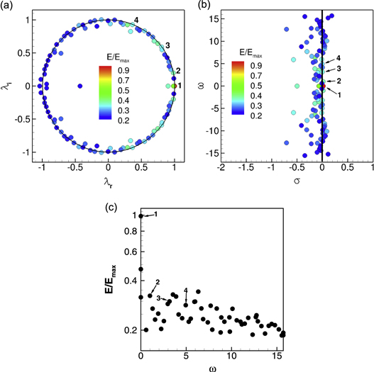
Figure 7. PIV data at the junction of the TCPC: eigenvalues (a)–(b) and spectrum (c).
Download figure:
Standard image High-resolution imageFigure 8 shows the out-of-plane velocity component for the four selected eigenmodes. Figure 8(a) shows a positive contour on the top part and a negative contour on the bottom part which consistent with the presence of a unique vortex rotating clockwise at the junction. Figure 8(b) shows a similar pattern, but with the negative contour on the top part of the domain and the positive contour on the bottom part of the domain, indicating the presence of a unique vortex, this time rotating in the opposite direction. Figure 8(c) shows a pattern with positive/negative/positive profile along the y-direction, which is consistent with the presence of two counter rotating vortices inside the pulmonary arteries. Figure 8(d) shows a similar pattern as figure 8(c), but with an opposite sign.

Figure 8. PIV data: four selected DMD modes. The lengths have been non-dimensionalized by the VC diameter.
Download figure:
Standard image High-resolution imageDMD is then applied to LES data. Similarly to the experiments, data are only extracted at the center plane of the TCPC junction, with a constant sampling time of 0.2 s (hundred snapshots). The grid used for each snapshot contains 100 × 50 grid points and all three components of the velocity are used to build the data matrix  . The sampling rate and the grid used are similar to the ones used for the experiments, allowing comparison of the results with the ones obtained from the experimental data.
Figure 9(a) shows the eigenvalues colored by the normalized temporal coherence: the eigenvalues are more regularly distributed around the unit circle than the eigenvalues obtained from SPIV data, which consistent with the absence of noise in the data. Four modes are selected and identified for their high coherence. These same eigenvalues are highlighted on figure 9(b). Figure 9(c) shows the spectrum extracted from the LES data: it can be seen that the DMD extracts many different modes with distinct frequencies and temporal coherence. The four selected modes are shown in figure 10 as the out-of-plane component of the real velocity. Figure 10(a) shows a pattern consistent with a unique vortex at the junction of the TCPC. Figure 10(b) also shows a pattern consistent with the presence of a unique vortex, but rotating in the opposing direction. Figures 10(c) and (d) shows the presence of two counter rotating vortices. All these four modes are similar to the ones observed from the experimental data, which indicates agreement between simulations and measurements at the DMD level.

Figure 9. LES data at the junction of the TCPC: eigenvalues (a)–(b) and spectra (c).
Download figure:
Standard image High-resolution image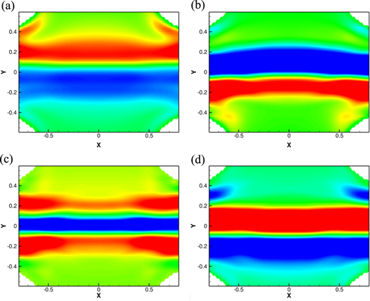
Figure 10. LES data: 4 selected DMD modes. The lengths have been non-dimensionalized by the VC diameter.
Download figure:
Standard image High-resolution image3.2.2. DMD of Fontan hemodynamics in an idealized TCPC with a 0.5D caval offset in the pulmonary arteries direction:
A typical solution used to reduce the energy losses induced by the unstable flow seen in the previous section is to offset the two VCs to prevent the two jets from directly colliding. We study here a case with a caval offset of 0.5 diameter along the pulmonary arteries. Figure 11 shows time variation of instantaneous flow features for this case. The flow structures are represented by iso-surfaces of  colored by vorticity magnitude. The flow field induced by this TCPC geometry is unstable: rotating flow structures (figures 11(a)–(c)) that are periodically washed out in the pulmonary arteries (figures 11(d)–(f)) are observed. This phenomenon occurs periodically and is due to the configuration of the VCs: the offset induces a rotation of the flow at the junction in the counter-clockwise direction in a PA/VC plane. But this rotation is not 'compatible' with the preferential rotation that is induced by the pulmonary arteries. The interaction of vortices is responsible for the instabilities observed. This phenomenom can be more easily seen on figure 12.

Figure 11. 0.5D caval offset: iso-surface of  colored by vorticity magnitude (
 ). The unstable interaction between the two VC jets can be seen at the junction of the TCPC, as well as in the pulmonary arteries.
Download figure:
Standard image High-resolution image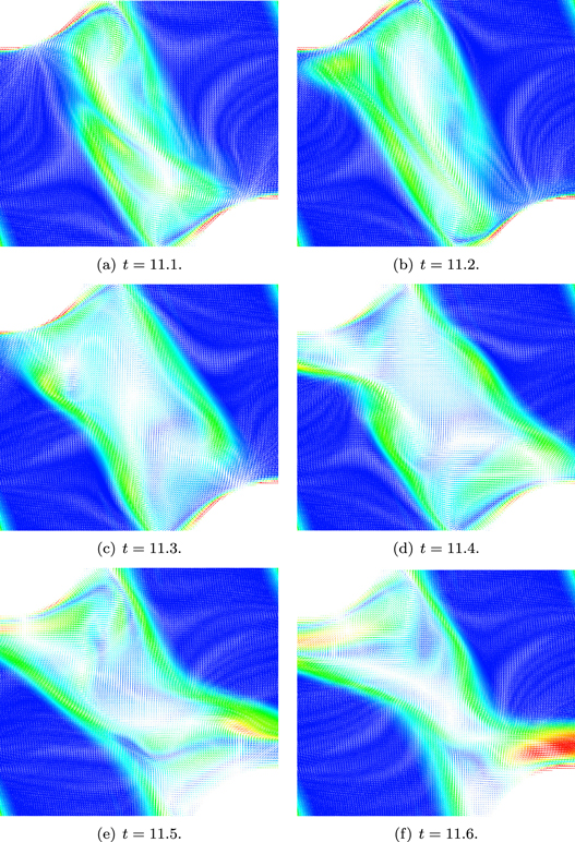
Figure 12. In-plane velocity vectors colored by vorticity magnitude at the junction of the TCPC. The interaction between the two shear layers is very unsteady, and recirculating flow can be seen at the junction of the TCPC.
Download figure:
Standard image High-resolution imageFigure 12 shows in plane velocity vectors colored by vorticity magnitude at the TCPC junction for different instant in time. Two shear layers coming from each VC are observed. These two shear layers prevent the flow coming from each VC to mix: even if the offset is only of 50%, it induces preferential distribution of the VC flow. The flow coming from the IVC mostly goes to the LPA and the flow coming from the SVC mostly goes to the RPA. Between the two shear layers, re-circulation of the flow is be observed: the two shear layers are interacting with each other and are unstable. The region shows high vorticity compared to the rest of the domain.
To perform the DMD analysis, a hundred samples of the flow field at the junction of the TCPC are extracted at a constant sampling time of 0.1 s, capturing about five periods of unstable flow structures. All three components of the velocity are used to build the data matrix  . Figure 13 shows the results of the DMD analysis. Figure 13(a) shows the complex eigenvalues colored by temporal coherence. Six eigenvalues are highlighted. Figures 13(b) and (c) show the logarithmic mapping of the eigenvalues, colored by temporal coherence. Most modes are stable (negative value of the growth rate). A few modes are unstable, but these modes are very noisy and are not considered here. All the considered modes are stable. Figure 13(c) shows the spectra obtained from the DMD analysis.
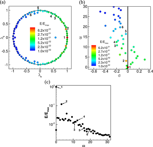
Figure 13. DMD of the TCPC with 0.5D caval offset: eigenvalues (a)–(b) and spectra (c).
Download figure:
Standard image High-resolution imageThe six selected DMD modes are shown on figure 14. Real out of plane vorticity is shown. Figure 14(a) shows the first mode, which is equivalent to the mean flow. The preferential path of the flow coming from both the SVC and IVC is observed. This is consistent with the flow pattern seen on the instantaneous snapshots. Figure 14(b) shows the second extracted mode. A main vortex consistent with the re-circulation zone between the two shear layers is observed. Modes 3, 4, 5 and 6 (figures 14(c)–(f)) highlight smaller and smaller vortical structures. The small vortices are rotating both clockwise and counter-clockwise and the shape of the high velocity region is clearly seen. It is parallel to the two shear layers, approximately 45 degs towards the top left corner. The DMD analysis allows the extraction of the main modes (mean, and re-circulation zones), as well as to show the complex interaction of the two jets at the junction. The presence of smaller and smaller vortices are consistent with the spectra shown in figure 13(c).

Figure 14. 0.5D offset: six selected DMD modes (out of plane vorticity). Mode 1 (a) is similar to the mean flow showing the bifurcation of the flow coming from both vena cavae into the pulmonary arteries, whereas the other modes (b)–(f) show vortical structures of different scales. The lengths have been non-dimensionalized by the VC diameter.
Download figure:
Standard image High-resolution image
4. Conclusion
LES and SPIV show that a swirl switching phenomenon happens in TCPC geometries. Vortices with different signs are successively present in the pulmonary arteries [11, 12]. Because of the periodic change of sign, LES data show a zero mean out of plane velocity. However SPIV data result in mean profiles showing a helical pattern, indicating that the experiments mostly capture one of the rotations. Instantaneous experimental data still contain information about this swirl switching phenomenon and the DMD analysis enables to highlight this. At the DMD level, LES and SPIV are in excellent agreement and show similar flow features. Four of the main modes selected in this study show the change of sign of the rotation, as well as the periodic presence of the two vortices inside the pulmonary arteries. When applied to the geometry with caval offset, the DMD analysis allowed for the visualization of the preferential direction of the flow, as well as the shape of the main shear layer that divides the streams coming from the IVC and SVC. In conclusion DMD analysis is a valuable tool to extract and study particular flow fields, especially in the presence of instabilities that makes mean flow less meaningful.
Acknowledgments
The authors would like to acknowledge financial support for this work by the National Institute of Health (NIH) (Grant no. HL098353) and by an American Heart Association Predoctoral Fellowship (11PRE7840073) (AEK).