
Modeling Soil Moisture from Multisource Data by Stepwise Multilinear Regression: An Application to the Chinese Loess Plateau

 ,
,  ,
, 
Abstract
:1. Introduction
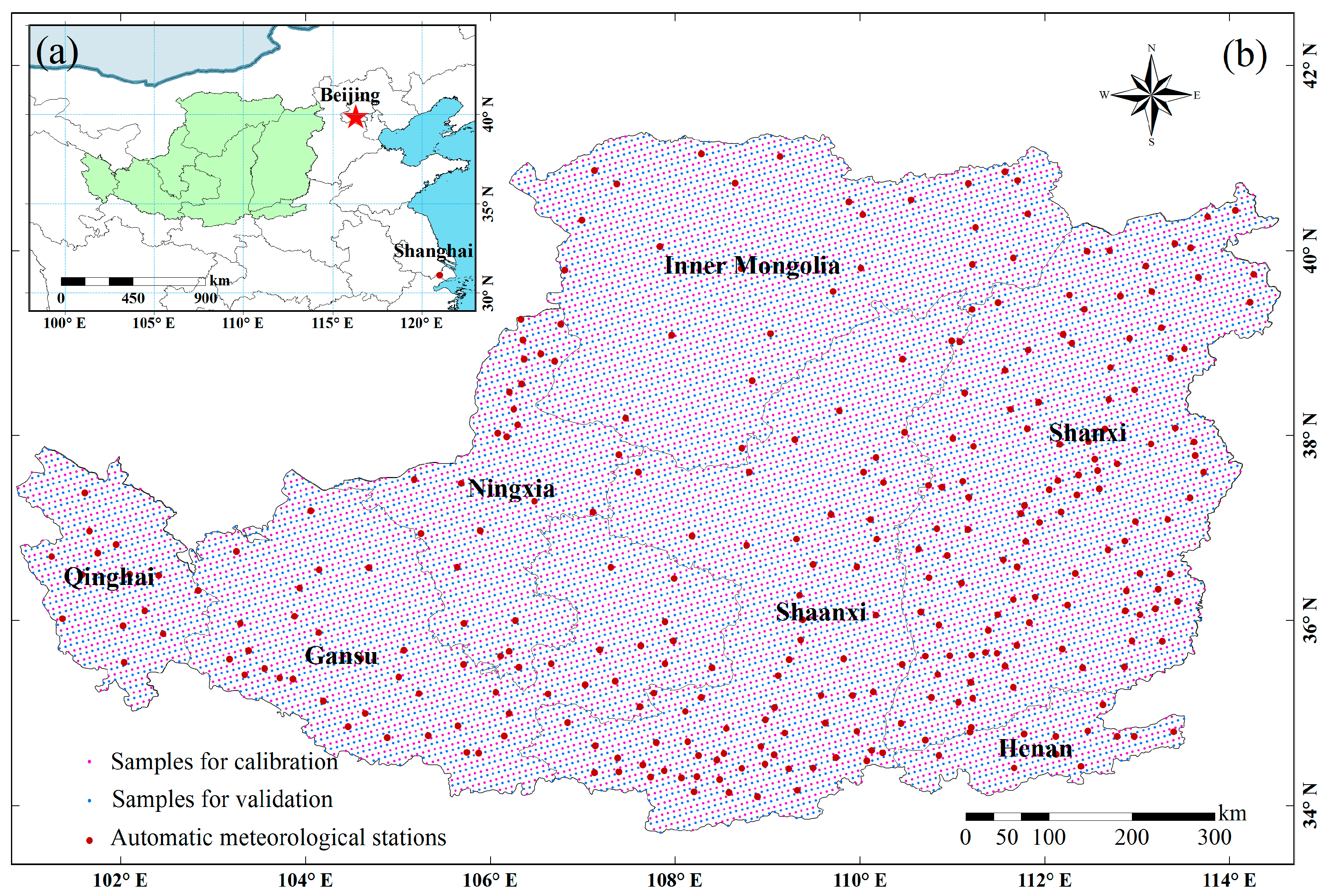
2. Study Area
3. Materials and Methods
3.1. Soil Moisture Data
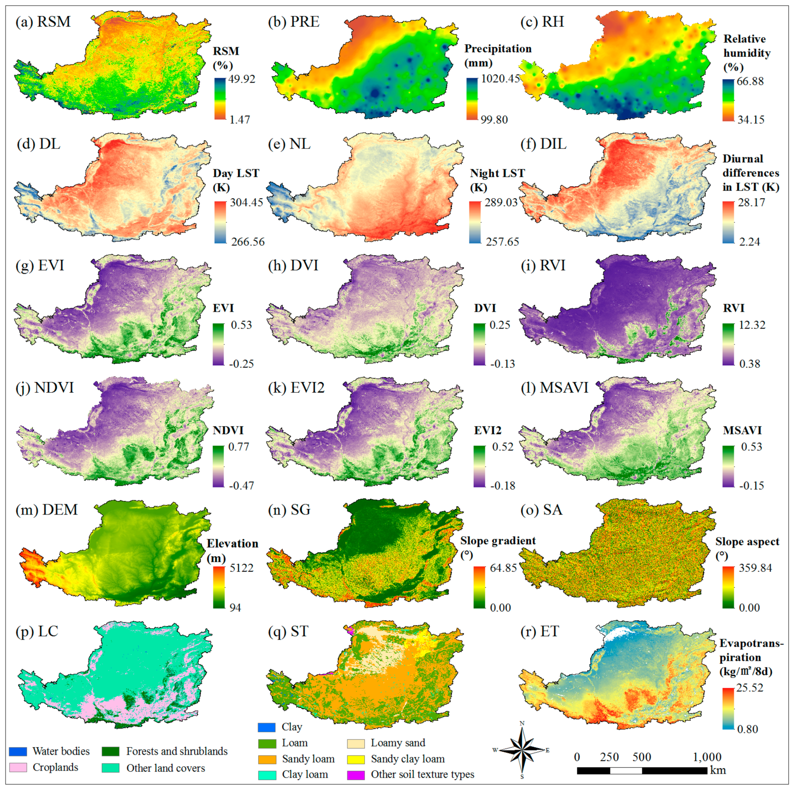
3.2. Candidate Variables
3.2.1. MODIS Data
3.2.2. Topographic Data
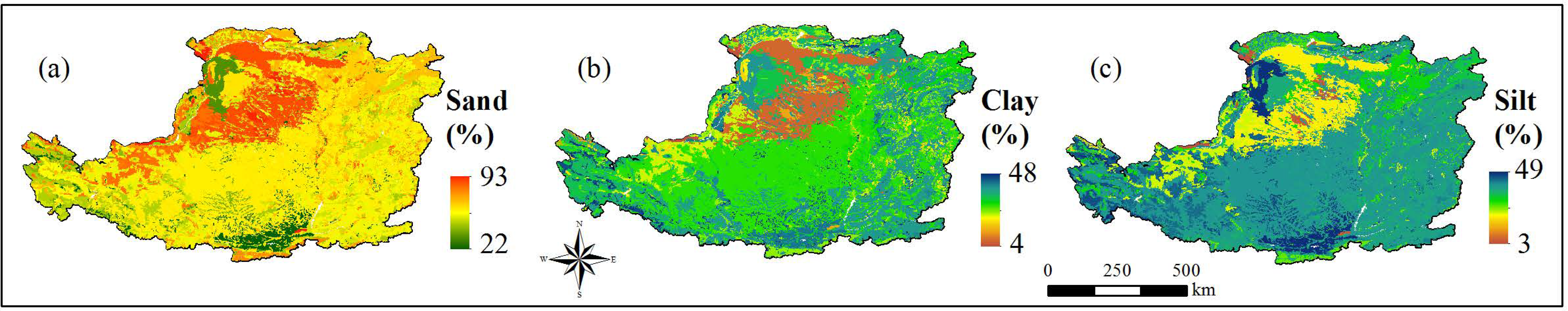
3.2.3. Soil Properties Data
3.2.4. Meteorological Data
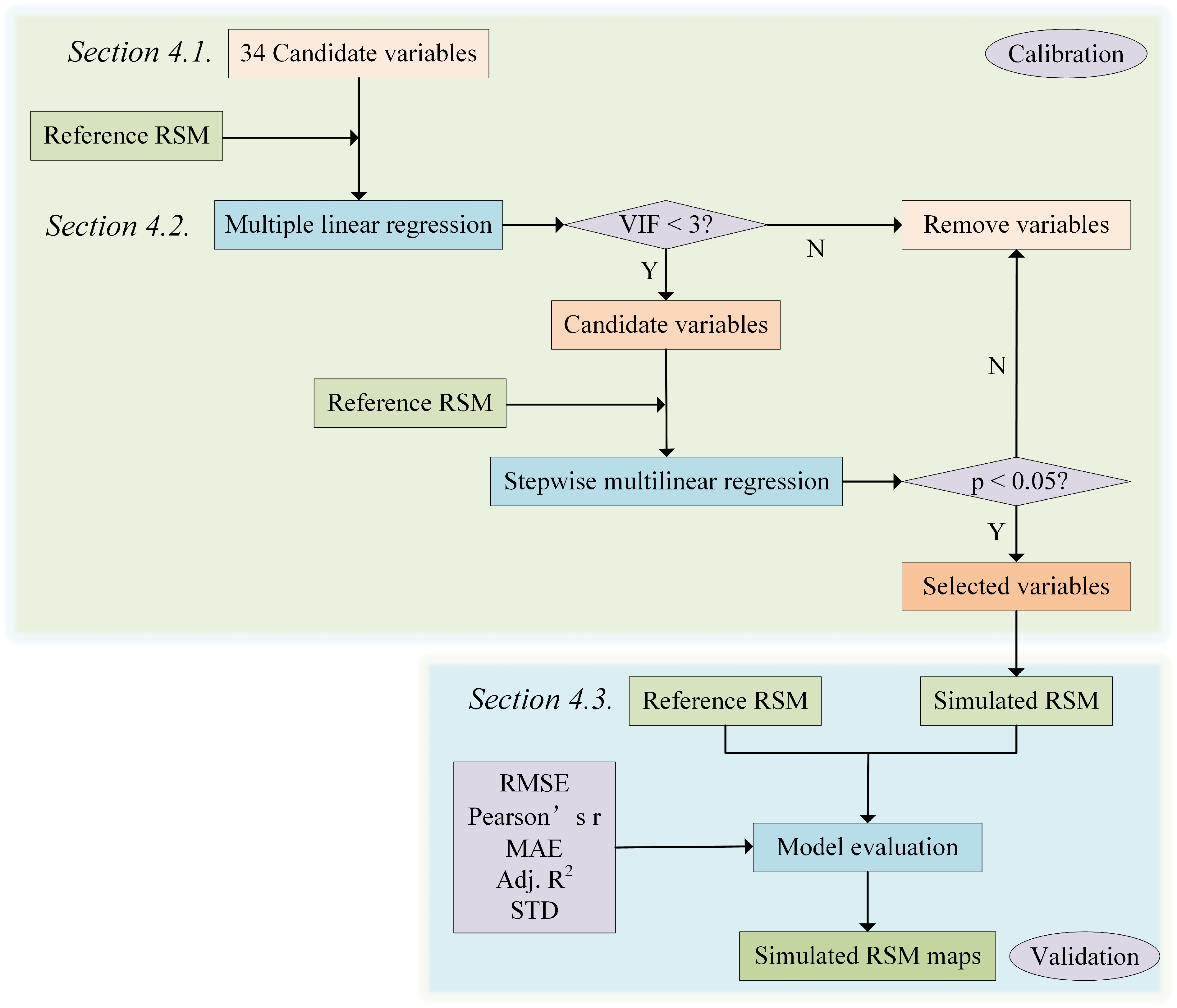
3.3. Stepwise Multilinear Regression Modeling
3.4. Accuracy Assessment
4. Results
4.1. Stepwise Multilinear Regression Model
4.2. Accuracy Assessment
4.3. Modeled Soil Moisture
5. Discussion
6. Conclusions
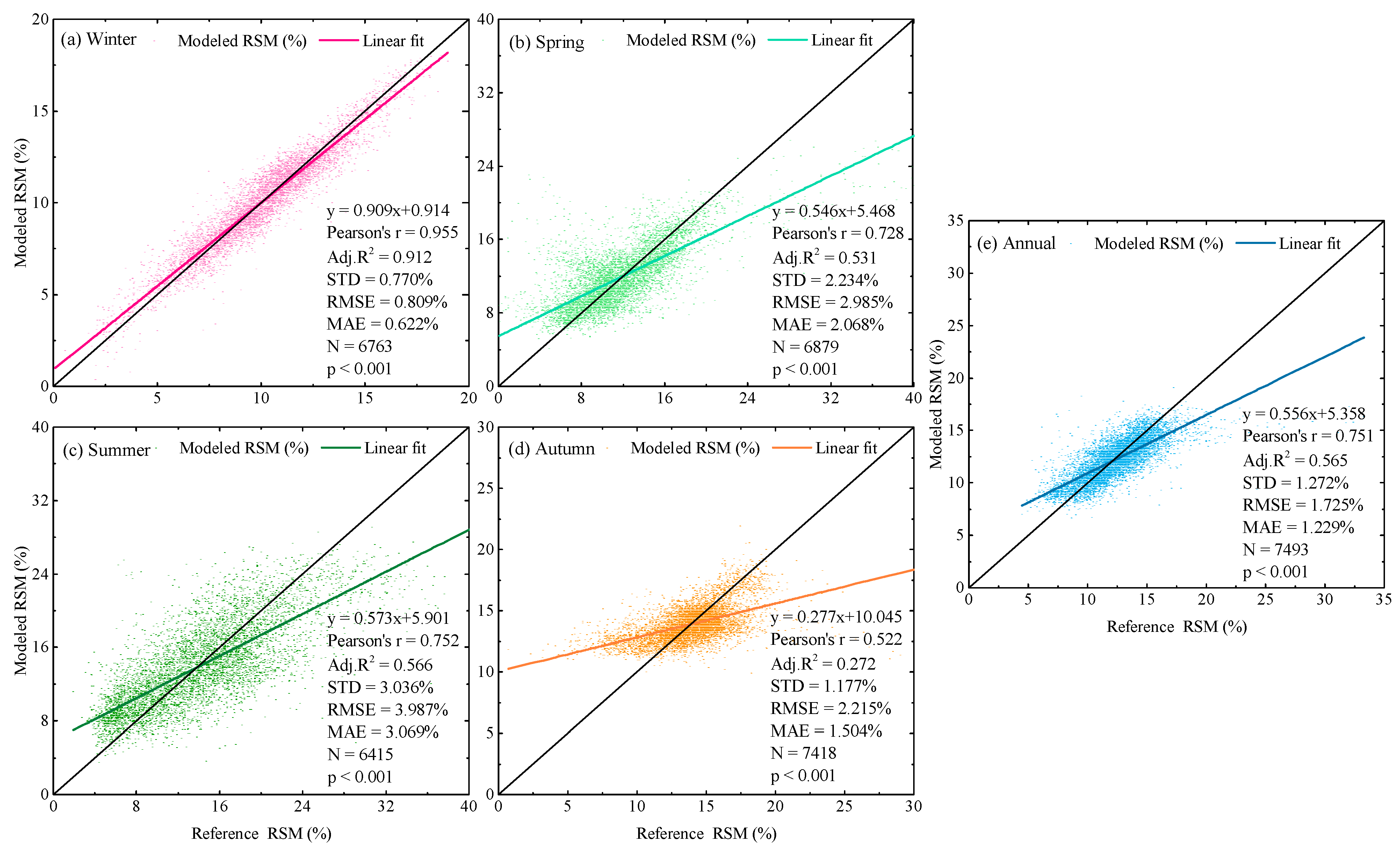
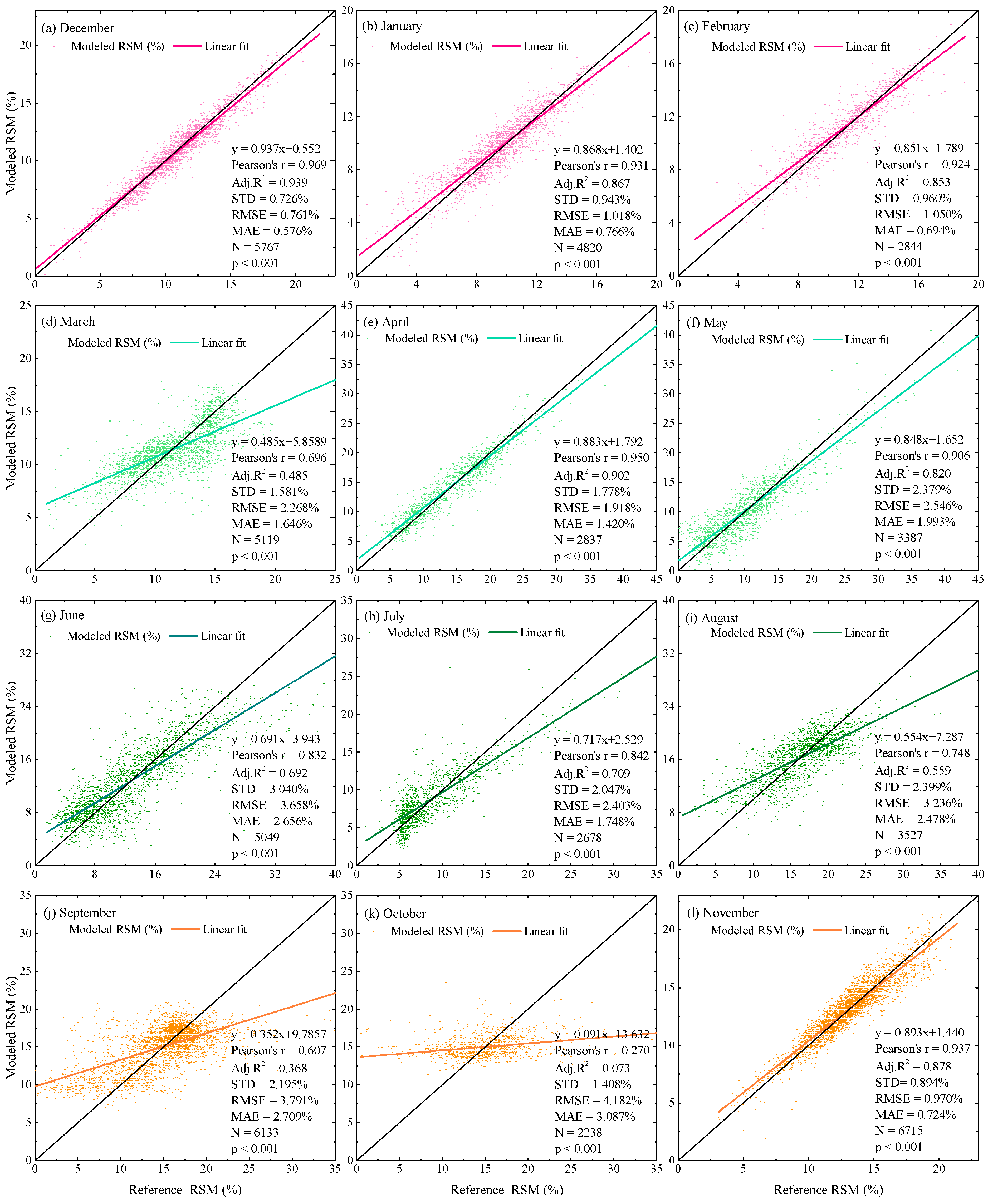
- SMLR could model RSM with the desired accuracy (r = 0.969, RMSE = 0.761%, MAE = 0.576% in December) at a 500 m resolution over the CLP. Moreover, the use of multisource data to complement and/or replace coarse-resolution satellite data in RSM modeling could be considered.
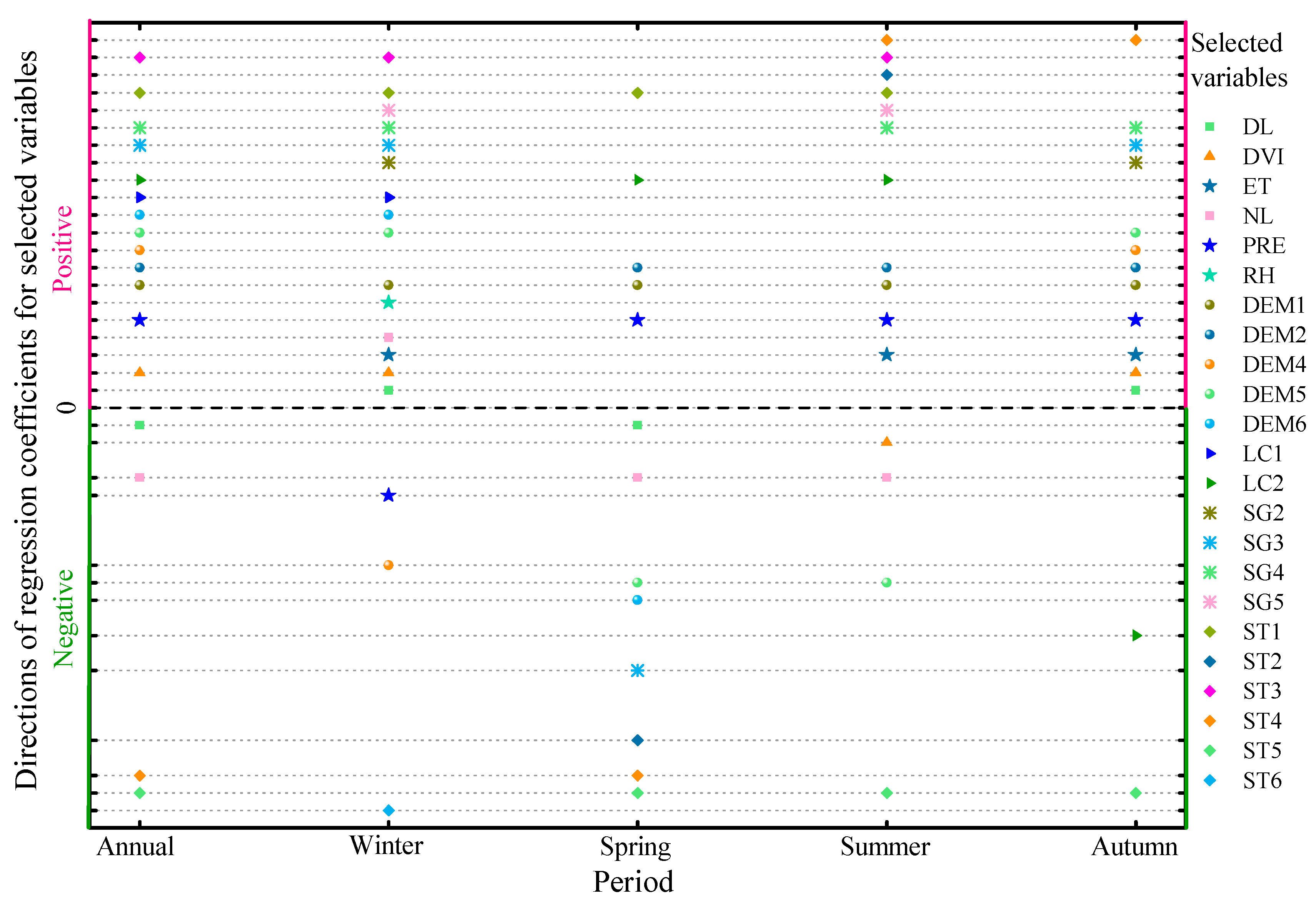
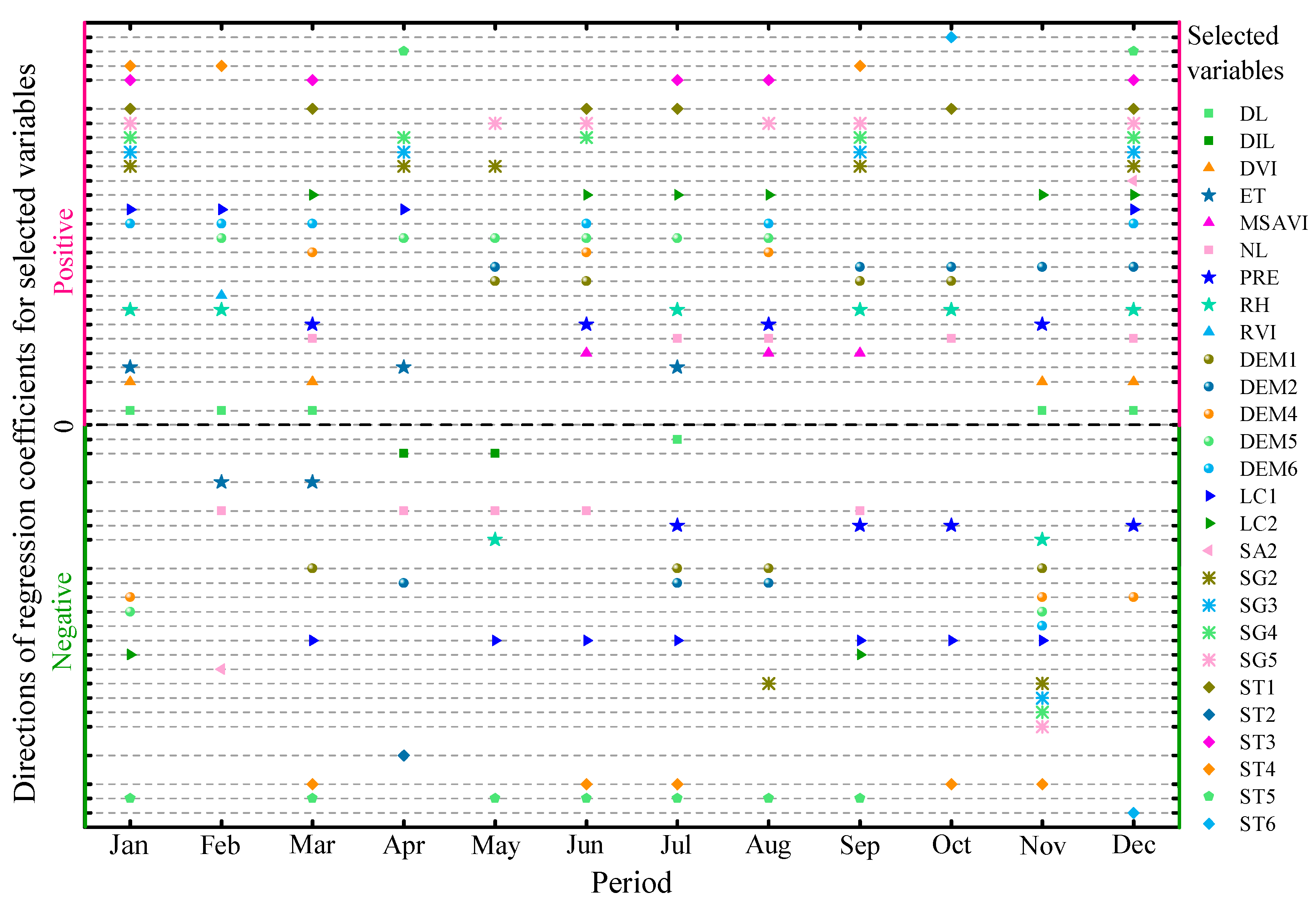
- The variables of elevation (0–500 m and 2000–2500 m), precipitation, soil texture of the loam, and nighttime land surface temperature could continuously be used in the regression models for all seasons in 2017.
- Including dummy variables improved the model fit, both in calibration and validation, because the Adj. R2 was higher with dummy variables than without.
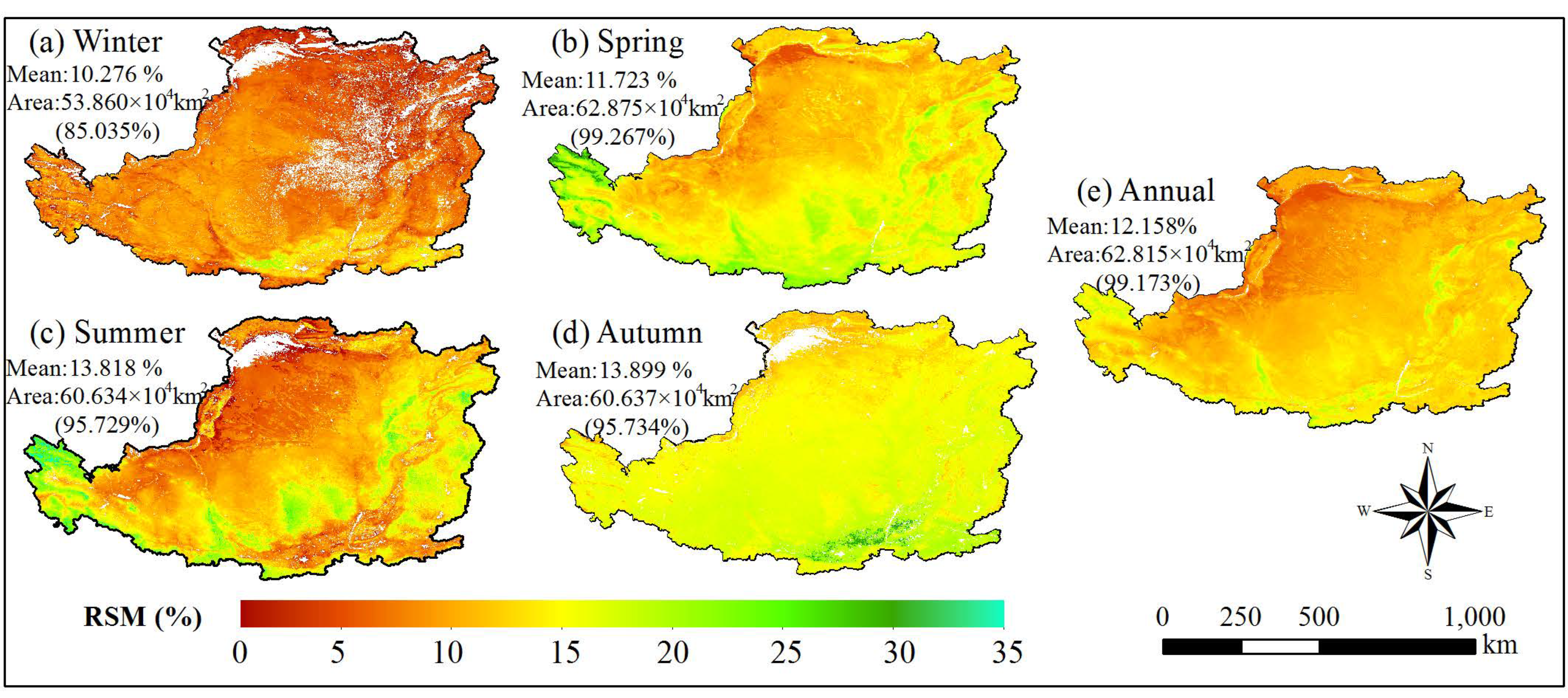
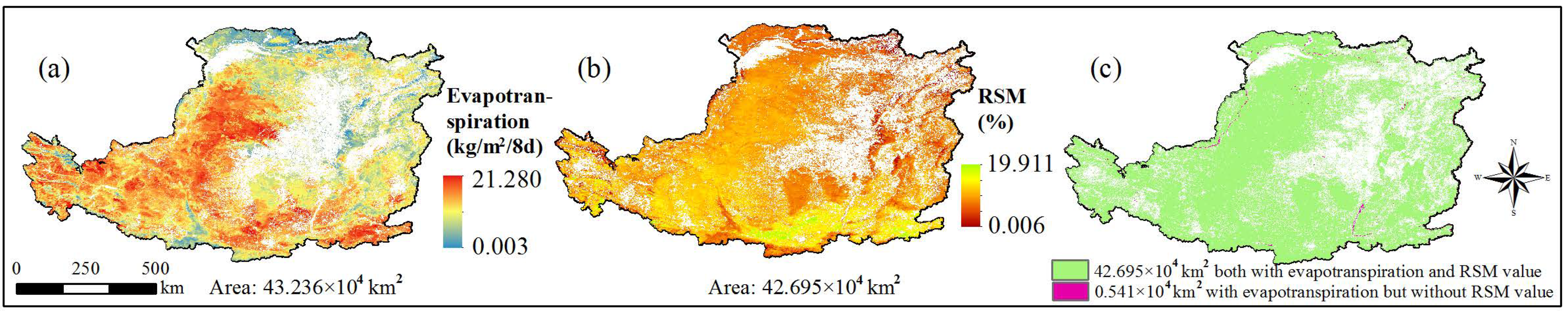
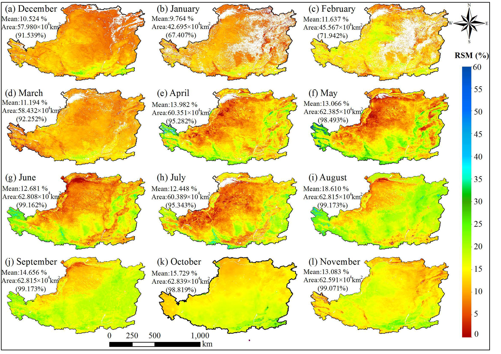
- The SMLR-modeled RSM for almost all periods except for January and February (because of unavailable ET data at that time) achieved better spatial coverage than that of the reference RSM. Thus, the availability of selected variables directly affects the coverage of the modeled RSM.
Author Contributions
Funding
Institutional Review Board Statement
Informed Consent Statement
Data Availability Statement
Acknowledgments
Conflicts of Interest
Appendix A


Appendix B

| Period | Validation Results | Reference RSM | ||||
|---|---|---|---|---|---|---|
| r | Adj. R2 | MAE (%) | RMSE (%) | Mean RSM (%) | Area (104 km2) | |
| Annual | 0.73 | 0.52 | 3.00 | 3.75 | 10.16 | 63.24 |
| Winter | 0.67 | 0.44 | 3.22 | 3.74 | 9.08 | 60.90 |
| Spring | 0.53 | 0.27 | 3.14 | 3.98 | 11.68 | 58.00 |
| Summer | 0.58 | 0.34 | 3.25 | 3.86 | 13.82 | 54.57 |
| Autumn | 0.67 | 0.44 | 3.64 | 4.41 | 13.91 | 61.99 |
| January | 0.68 | 0.45 | 3.24 | 4.06 | 9.31 | 56.18 |
| February | 0.66 | 0.42 | 3.23 | 3.84 | 8.64 | 62.39 |
| March | 0.57 | 0.32 | 3.02 | 3.91 | 11.42 | 42.92 |
| April | 0.64 | 0.41 | 3.09 | 3.77 | 14.18 | 24.93 |
| May | 0.65 | 0.42 | 3.27 | 3.89 | 10.50 | 29.26 |
| June | 0.59 | 0.35 | 3.81 | 4.54 | 12.83 | 43.44 |
| July | 0.54 | 0.28 | 3.43 | 4.29 | 8.85 | 24.16 |
| August | 0.61 | 0.37 | 3.62 | 4.48 | 16.42 | 29.20 |
| September | 0.57 | 0.32 | 3.58 | 4.57 | 14.91 | 51.91 |
| October | 0.47 | 0.21 | 4.97 | 6.10 | 15.05 | 18.32 |
| November | 0.50 | 0.25 | 3.80 | 4.66 | 13.03 | 61.01 |
| December | 0.64 | 0.40 | 3.26 | 3.99 | 10.72 | 56.96 |
| Vegetation Index | Formula |
|---|---|
| Enhanced vegetation index (EVI) | |
| Difference vegetation index (DVI) | |
| Ratio vegetation index (RVI) | |
| Normalized difference vegetation index (NDVI) | |
| Enhanced vegetation index 2 (EVI2) | |
| Modified soil-adjusted vegetation index (MSAVI) |
| Abbreviation | Formula 1 |
|---|---|
| RMSE | |
| r | |
| MAE | |
| R2 | |
| STD |
| Period | Regression Model | Adj. R2 | RMSE | Max VIF |
|---|---|---|---|---|
| January | RSM = −243.006 + 0.900*DL + 15.761*DVI + 0.150*ET + 0.021*RH − 0.350*DEM4 − 0.153*DEM5 + 0.508*DEM6 + 0.285*LC1 − 0.630*LC2 + 0.275*SG2 + 0.448*SG3 + 0.423*SG4 + 0.513*SG5 + 0.170*ST1 + 0.816*ST3 + 0.529*ST4 − 0.221*ST5 | 0.864 | 1.016 | 1.884 |
| February | RSM = −165.850 + 0.688*DL − 0.059*ET − 0.072*NL + 0.031*RH + 0.502*RVI + 0.341*DEM5 + 0.442*DEM6 + 0.214*LC1 − 0.104*SA2 + 0.338*ST4 | 0.849 | 1.034 | 1.733 |
| March | RSM = −139.430 + 0.431*DL + 20.424*DVI − 0.144*ET + 0.096*NL + 0.033*PRE − 0.375*DEM1 + 0.426*DEM4 + 1.114*DEM6 − 0.433*LC1 + 3.674*LC2 + 0.266*ST1 + 2.537*ST3 − 1.147*ST4 − 1.191*ST5 | 0.467 | 2.317 | 2.382 |
| April | RSM = 257.901 − 1.070*DIL + 0.183*ET − 0.803*NL − 0.152*DEM2 + 0.179*DEM5 + 0.620*LC1 + 0.414*SG2 + 0.769*SG3 + 0.673*SG4 − 1.131*ST2 + 0.577*ST5 | 0.899 | 1.892 | 2.138 |
| May | RSM = 361.380 − 1.130*DIL − 1.132*NL − 0.078*RH + 1.072*DEM1 + 0.502*DEM2 + 0.420*DEM5 − 0.277*LC1 + 0.276*SG2 + 0.512*SG5 − 1.039*ST5 | 0.823 | 2.545 | 1.938 |
| June | RSM = 222.274 + 19.787*MSAVI − 0.764*NL + 0.044*PRE + 0.813*DEM1 + 0.539*DEM4 + 0.863*DEM5 + 1.460*DEM6 − 0.437*LC1 + 4.148*LC2 + 0.387*SG4 + 0.989*SG5 + 0.396*ST1 − 3.075*ST4 − 1.648*ST5 | 0.708 | 3.528 | 1.993 |
| July | RSM = 160.019 − 0.648*DL + 0.141*ET + 0.154*NL − 0.016*PRE + 0.116*RH − 1.260*DEM1 − 0.585*DEM2 + 0.393*DEM5 − 0.622*LC1 + 2.584*LC2 + 0.233*ST1 + 5.579*ST3 − 0.853*ST4 − 0.368*ST5 | 0.694 | 2.434 | 2.604 |
| August | RSM = 167.362 + 19.965*MSAVI − 0.548*NL + 0.018*PRE − 1.666*DEM1 − 0.865*DEM2 + 1.372*DEM4 + 1.845*DEM5 + 1.297*DEM6 + 2.000*LC2 − 0.314*SG2 + 0.618*SG5 + 9.771*ST3 − 1.965*ST5 | 0.560 | 3.197 | 2.856 |
| September | RSM = 83.292 + 13.956*MSAVI − 0.278*NL − 0.006*PRE + 0.079*RH + 3.487*DEM1 + 1.625*DEM2 − 0.575*LC1 − 2.252*LC2 + 0.866*SG2 + 0.669*SG3 + 0.789*SG4 + 0.470*SG5 + 1.810*ST4 − 0.866*ST5 | 0.334 | 3.926 | 2.841 |
| October | RSM = −31.338 + 0.124*NL − 0.023*PRE + 0.191*RH + 3.825*DEM1 + 0.923*DEM2 − 0.817*LC1 + 0.505*ST1 − 0.913*ST4 + 9.032*ST6 | 0.091 | 4.182 | 1.592 |
| November | RSM = −255.132 + 0.948*DL + 8.246*DVI + 0.021*PRE − 0.007*RH − 0.429*DEM1 + 0.100*DEM2 − 0.342*DEM4 − 0.423*DEM5 − 0.203*DEM6 − 0.196*LC1 + 0.238*LC2 − 0.177*SG2 − 0.137*SG3 − 0.166*SG4 − 0.144*SG5 − 0.421*ST4 | 0.880 | 0.938 | 2.345 |
| December | RSM = −274.446 + 0.999*DL + 21.603*DVI + 0.021*NL − 0.036*PRE + 0.020*RH + 0.125*DEM2 − 0.163*DEM4 + 0.137*DEM6 + 0.069*LC1 + 0.617*LC2 + 0.052*SA2 + 0.122*SG2 + 0.152*SG3 + 0.203*SG4 + 0.121*SG5 + 0.065*ST1 + 0.875*ST3 + 0.219*ST5 − 0.846*ST6 | 0.938 | 0.753 | 2.293 |
References
- Albertson, J.D.; Kiely, G. On the structure of soil moisture time series in the context of land surface models. J. Hydrol. 2001, 243, 101–119. [Google Scholar] [CrossRef]
- Spennemann, P.C.; Salvia, M.; Ruscica, R.C.; Sörensson, A.A.; Grings, F.; Karszenbaum, H. Land-atmosphere interaction patterns in southeastern South America using satellite products and climate models. Int. J. Appl. Earth Obs. Geoinf. 2018, 64, 96–103. [Google Scholar] [CrossRef]
- Tayfur, G.; Zucco, G.; Brocca, L.; Moramarco, T. Coupling soil moisture and precipitation observations for predicting hourly runoff at small catchment scale. J. Hydrol. 2014, 510, 363–371. [Google Scholar] [CrossRef] [Green Version]
- Zhang, B.; Aghakouchak, A.; Yang, Y.; Wei, J.; Wang, G. A water-energy balance approach for multi-category drought assessment across globally diverse hydrological basins. Agric. For. Meteorol. 2019, 264, 247–265. [Google Scholar] [CrossRef]
- Dorigo, W.; de Jeu, R. Satellite soil moisture for advancing our understanding of earth system processes and climate change. Int. J. Appl. Earth Obs. Geoinf. 2016, 48, 1–4. [Google Scholar] [CrossRef]
- Kumar, S.V.; Dirmeyer, P.A.; Peters-Lidard, C.D.; Bindlish, R.; Bolten, J. Information theoretic evaluation of satellite soil moisture retrievals. Remote Sens. Environ. 2018, 204, 392–400. [Google Scholar] [CrossRef] [Green Version]
- Liu, D.; Mishra, A.K.; Yu, Z.; Yang, C.; Konapala, G.; Vu, T. Performance of SMAP, AMSR-E and LAI for weekly agricultural drought forecasting over continental United States. J. Hydrol. 2017, 553, 88–104. [Google Scholar] [CrossRef]
- Kim, S.; Zhang, R.; Pham, H.; Sharma, A. A review of satellite-derived soil moisture and its usage for flood estimation. Remote Sens. Earth Syst. Sci. 2019, 2, 225–246. [Google Scholar] [CrossRef]
- Singh, A.K.; Bhardwaj, A.K.; Verma, C.L.; Mishra, V.K. Soil moisture sensing techniques for scheduling irrigation. J. Soil Salin. Water Qual. 2019, 11, 68–76. [Google Scholar]
- Zaussinger, F.; Dorigo, W.; Gruber, A.; Tarpanelli, A.; Filippucci, P.; Brocca, L. Estimating irrigation water use over the contiguous United States by combining satellite and reanalysis soil moisture data. Hydrol. Earth Syst. Sci. 2019, 23, 897–923. [Google Scholar] [CrossRef] [Green Version]
- Yuan, L.; Li, L.; Zhang, T.; Chen, L.; Zhao, J.; Hu, S.; Cheng, L.; Liu, W. Soil moisture estimation for the Chinese Loess Plateau using MODIS-derived ATI and TVDI. Remote Sens. 2020, 12, 3040. [Google Scholar] [CrossRef]
- Fang, B.; Lakshmi, V. Soil moisture at watershed scale: Remote sensing techniques. J. Hydrol. 2014, 516, 258–272. [Google Scholar] [CrossRef]
- Ma, H.; Zhang, L.; Sun, L.; Liu, Q. Farmland soil moisture inversion by synergizing optical and microwave remote sensing data. J. Remote Sens. 2014, 18, 673–685. [Google Scholar] [CrossRef]
- Karthikeyan, L.; Pan, M.; Wanders, N.; Kumar, D.N.; Wood, E.F. Four decades of microwave satellite soil moisture observations: Part 2. Product validation and inter-satellite comparisons. Adv. Water Resour. 2017, 109, 236–252. [Google Scholar] [CrossRef]
- Djamai, N.; Magagi, R.; Goïta, K.; Merlin, O.; Kerr, Y.; Roy, A. A combination of DISPATCH downscaling algorithm with CLASS land surface scheme for soil moisture estimation at fine scale during cloudy days. Remote Sens. Environ. 2016, 184, 1–14. [Google Scholar] [CrossRef]
- Piles, M.; Ballabrera-Poy, J.; Muñoz-Sabater, J. Dominant features of global surface soil moisture variability observed by the SMOS satellite. Remote Sens. 2019, 11, 95. [Google Scholar] [CrossRef] [Green Version]
- Doubková, M.; van Dijk, A.I.J.M.; Sabel, D.; Wagner, W.; Blöschl, G. Evaluation of the predicted error of the soil moisture retrieval from C-band SAR by comparison against modelled soil moisture estimates over Australia. Remote Sens. Environ. 2012, 120, 188–196. [Google Scholar] [CrossRef] [Green Version]
- Han, J.; Mao, K.; Xu, T.; Guo, J.; Zuo, Z.; Gao, C. A soil moisture estimation framework based on the CART algorithm and its application in China. J. Hydrol. 2018, 563, 65–75. [Google Scholar] [CrossRef]
- Dumedah, G.; Walker, J.P. Intercomparison of the JULES and CABLE land surface models through assimilation of remotely sensed soil moisture in southeast Australia. Adv. Water Resour. 2014, 74, 231–244. [Google Scholar] [CrossRef]
- Moon, H.; Choi, M. Dryness indices based on remotely sensed vegetation and land surface temperature for evaluating the soil moisture status in cropland-forest-dominant watersheds. Terr. Atmos. Ocean. Sci. 2015, 26, 599–611. [Google Scholar] [CrossRef] [Green Version]
- Malbéteau, Y.; Merlin, O.; Molero, B.; Rüdiger, C.; Bacon, S. DisPATCh as a tool to evaluate coarse-scale remotely sensed soil moisture using localized in situ measurements: Application to SMOS and AMSR-E data in Southeastern Australia. Int. J. Appl. Earth Obs. Geoinf. 2016, 45, 221–234. [Google Scholar] [CrossRef]
- Djamai, N.; Magagi, R.; Goita, K.; Merlin, O.; Kerr, Y.; Walker, A. Disaggregation of SMOS soil moisture over the Canadian Prairies. Remote Sens. Environ. 2015, 170, 255–268. [Google Scholar] [CrossRef] [Green Version]
- Tagesson, T.; Horion, S.; Nieto, H.; Zaldo Fornies, V.; Mendiguren González, G.; Bulgin, C.E.; Ghent, D.; Fensholt, R. Disaggregation of SMOS soil moisture over West Africa using the Temperature and Vegetation Dryness Index based on SEVIRI land surface parameters. Remote Sens. Environ. 2018, 206, 424–441. [Google Scholar] [CrossRef] [Green Version]
- Merlin, O.; Malbéteau, Y.; Notfi, Y.; Bacon, S.; Er-raki, S. Performance metrics for soil moisture downscaling methods: Application to DISPATCH data in Central Morocco. Remote Sens. 2015, 7, 3783–3807. [Google Scholar] [CrossRef] [Green Version]
- Zhang, D.; Zhou, G. Estimation of soil moisture from optical and thermal remote sensing: A review. Sensors 2016, 16, 1308. [Google Scholar] [CrossRef] [Green Version]
- Liu, Y.; Qian, J.; Yue, H. Combined Sentinel-1A with Sentinel-2A to estimate soil moisture in farmland. IEEE J. Sel. Top. Appl. Earth Obs. Remote Sens. 2021, 14, 1292–1310. [Google Scholar] [CrossRef]
- Koley, S.; Jeganathan, C. Estimation and evaluation of high spatial resolution surface soil moisture using multi-sensor multi-resolution approach. Geoderma 2020, 378, 114618. [Google Scholar] [CrossRef]
- Palombo, A.; Pascucci, S.; Loperte, A.; Lettino, A.; Castaldi, F.; Muolo, M.R.; Santini, F. Soil moisture retrieval by integrating TASI-600 airborne thermal data, WorldView 2 satellite data and field measurements: Petacciato case study. Sensors 2019, 19, 1515. [Google Scholar] [CrossRef] [PubMed] [Green Version]
- Wang, H.; He, N.; Zhao, R.; Ma, X. Soil water content monitoring using joint application of PDI and TVDI drought indices. Remote Sens. Lett. 2020, 11, 455–464. [Google Scholar] [CrossRef]
- Lu, X.J.; Zhou, B.; Yan, H.B.; Luo, L.; Huang, Y.H.; Wu, C.L. Remote sensing retrieval of soil moisture in Guangxi based on ATI and TVDI models. Int. Arch. Photogramm. Remote Sens. Spat. Inf. Sci. ISPRS Arch. 2020, 42, 895–902. [Google Scholar] [CrossRef] [Green Version]
- Lu, L.; Luo, G.P.; Wang, J.Y. Development of an ATI-NDVI method for estimation of soil moisture from MODIS data. Int. J. Remote Sens. 2014, 35, 3797–3815. [Google Scholar] [CrossRef]
- Yuan, L.; Li, L.; Zhang, T.; Chen, L.; Zhao, J.; Liu, W.; Cheng, L.; Hu, S.; Yang, L.; Wen, M. Improving soil moisture estimation by identification of NDVI thresholds optimization: An application to the Chinese Loess Plateau. Remote Sens. 2021, 13, 589. [Google Scholar] [CrossRef]
- Sabaghy, S.; Walker, J.P.; Renzullo, L.J.; Jackson, T.J. Spatially enhanced passive microwave derived soil moisture: Capabilities and opportunities. Remote Sens. Environ. 2018, 209, 551–580. [Google Scholar] [CrossRef]
- Rahimi-Ajdadi, F.; Abbaspour-Gilandeh, Y.; Mollazade, K.; Hasanzadeh, R.P.R. Development of a novel machine vision procedure for rapid and non-contact measurement of soil moisture content. Meas. J. Int. Meas. Confed. 2018, 121, 179–189. [Google Scholar] [CrossRef]
- Sandells, M.J.; Davenport, I.J.; Gurney, R.J. Passive L-band microwave soil moisture retrieval error arising from topography in otherwise uniform scenes. Adv. Water Resour. 2008, 31, 1433–1443. [Google Scholar] [CrossRef]
- Fu, B.; Wang, J.; Chen, L.; Qiu, Y. The effects of land use on soil moisture variation in the Danangou catchment of the Loess Plateau, China. Catena 2003, 54, 197–213. [Google Scholar] [CrossRef]
- Niu, C.Y.; Musa, A.; Liu, Y. Analysis of soil moisture condition under different land uses in the arid region of Horqin sandy land, northern China. Solid Earth 2015, 6, 1157–1167. [Google Scholar] [CrossRef] [Green Version]
- Jiao, L.; Lu, N.; Fu, B.; Wang, J.; Li, Z.; Fang, W.; Liu, J.; Wang, C.; Zhang, L. Evapotranspiration partitioning and its implications for plant water use strategy: Evidence from a black locust plantation in the semi-arid Loess Plateau, China. For. Ecol. Manag. 2018, 424, 428–438. [Google Scholar] [CrossRef]
- Maheu, A.; Anctil, F.; Gaborit, É.; Fortin, V.; Nadeau, D.F.; Therrien, R. A field evaluation of soil moisture modelling with the Soil, Vegetation, and Snow (SVS) land surface model using evapotranspiration observations as forcing data. J. Hydrol. 2018, 558, 532–545. [Google Scholar] [CrossRef]
- Xu, Q.; Zhou, B. Retrieving soil water contents from soil temperature measurements by using linear regression. Adv. Atmos. Sci. 2003, 20, 849–858. [Google Scholar] [CrossRef]
- Wang, Y.; Shao, M.; Zhu, Y.; Sun, H.; Fang, L. A new index to quantify dried soil layers in water-limited ecosystems: A case study on the Chinese Loess Plateau. Geoderma 2018, 322, 1–11. [Google Scholar] [CrossRef]
- Li, X.; Xu, X.; Liu, W.; He, L.; Zhang, R.; Xu, C.; Wang, K. Similarity of the temporal pattern of soil moisture across soil profile in karst catchments of southwestern China. J. Hydrol. 2017, 555, 659–669. [Google Scholar] [CrossRef]
- Abowarda, A.S.; Bai, L.; Zhang, C.; Long, D.; Li, X.; Huang, Q.; Sun, Z. Generating surface soil moisture at 30 m spatial resolution using both data fusion and machine learning toward better water resources management at the field scale. Remote Sens. Environ. 2021, 255, 112301. [Google Scholar] [CrossRef]
- Khaki, M.; Zerihun, A.; Awange, J.L.; Dewan, A. Integrating satellite soil-moisture estimates and hydrological model products over Australia. Aust. J. Earth Sci. 2020, 67, 265–277. [Google Scholar] [CrossRef]
- Liu, D.; Mishra, A.K. Performance of AMSR_E soil moisture data assimilation in CLM4.5 model for monitoring hydrologic fluxes at global scale. J. Hydrol. 2017, 547, 67–79. [Google Scholar] [CrossRef] [Green Version]
- Zhao, L.; Yang, K.; Qin, J.; Chen, Y.; Tang, W.; Lu, H.; Yang, Z.L. The scale-dependence of SMOS soil moisture accuracy and its improvement through land data assimilation in the central Tibetan Plateau. Remote Sens. Environ. 2014, 152, 345–355. [Google Scholar] [CrossRef]
- Li, F.; Crow, W.T.; Kustas, W.P. Towards the estimation root-zone soil moisture via the simultaneous assimilation of thermal and microwave soil moisture retrievals. Adv. Water Resour. 2010, 33, 201–214. [Google Scholar] [CrossRef]
- Bayat, A.T.; Schonbrodt-Stitt, S.; Nasta, P.; Ahmadian, N.; Conrad, C.; Bogena, H.R.; Vereecken, H.; Jakobi, J.; Baatz, R.; Romano, N. Mapping near-surface soil moisture in a Mediterranean agroforestry ecosystem using Cosmic-Ray Neutron Probe and Sentinel-1 Data. In Proceedings of the 2020 IEEE International Workshop on Metrology for Agriculture and Forestry (MetroAgriFor), Trento, Italy, 4–6 November 2020; Volume 1, pp. 201–206. [Google Scholar] [CrossRef]
- Liu, Y.; Yao, L.; Jing, W.; Di, L.; Yang, J.; Li, Y. Comparison of two satellite-based soil moisture reconstruction algorithms: A case study in the state of Oklahoma, USA. J. Hydrol. 2020, 590, 125406. [Google Scholar] [CrossRef]
- Dumedah, G.; Walker, J.P.; Chik, L. Assessing artificial neural networks and statistical methods for infilling missing soil moisture records. J. Hydrol. 2014, 515, 330–344. [Google Scholar] [CrossRef]
- Santi, E.; Paloscia, S.; Pettinato, S.; Brocca, L.; Ciabatta, L.; Entekhabi, D. On the synergy of SMAP, AMSR2 and SENTINEL-1 for retrieving soil moisture. Int. J. Appl. Earth Obs. Geoinf. 2018, 65, 114–123. [Google Scholar] [CrossRef]
- Elshorbagy, A.; Parasuraman, K. On the relevance of using artificial neural networks for estimating soil moisture content. J. Hydrol. 2008, 362, 1–18. [Google Scholar] [CrossRef]
- Sharma, S.; Ochsner, T.E.; Twidwell, D.; Carlson, J.D.; Krueger, E.S.; Engle, D.M.; Fuhlendorf, S.D. Nondestructive estimation of standing crop and fuel moisture content in tallgrass prairie. Rangel. Ecol. Manag. 2018, 71, 356–362. [Google Scholar] [CrossRef]
- Zhang, X.; Chen, B.; Zhao, H.; Fan, H.; Zhu, D. Soil moisture retrieval over a semiarid area by means of PCA dimensionality reduction. Can. J. Remote Sens. 2016, 42, 136–144. [Google Scholar] [CrossRef]
- Pasolli, L.; Notarnicola, C.; Bruzzone, L.; Bertoldi, G.; Della Chiesa, S.; Niedrist, G.; Tappeiner, U.; Zebisch, M. Polarimetric RADARSAT-2 imagery for soil moisture retrieval in alpine areas. Can. J. Remote Sens. 2012, 37, 535–547. [Google Scholar] [CrossRef]
- Liu, D.; Mishra, A.K.; Yu, Z. Evaluating uncertainties in multi-layer soil moisture estimation with support vector machines and ensemble Kalman filtering. J. Hydrol. 2016, 538, 243–255. [Google Scholar] [CrossRef] [Green Version]
- Lee, Y.; Jung, C.; Kim, S. Spatial distribution of soil moisture estimates using a multiple linear regression model and Korean geostationary satellite (COMS) data. Agric. Water Manag. 2019, 213, 580–593. [Google Scholar] [CrossRef]
- Bortolini, D.; Albuquerque, J.A. Estimation of the retention and availability of water in soils of the State of Santa Catarina. Rev. Bras. Ciência Do Solo 2018, 42, 1–13. [Google Scholar] [CrossRef] [Green Version]
- Carranza, C.; Nolet, C.; Pezij, M.; Ploeg, M. Van Der Root zone soil moisture estimation with Random Forest. J. Hydrol. 2021, 593, 125840. [Google Scholar] [CrossRef]
- Gupta, D.K.; Prasad, R.; Kumar, P.; Vishwakarma, A.K. Soil moisture retrieval using ground based bistatic scatterometer data at X-band. Adv. Space Res. 2017, 59, 996–1007. [Google Scholar] [CrossRef]
- Chakravorty, A.; Chahar, B.R.; Sharma, O.P.; Dhanya, C.T. A regional scale performance evaluation of SMOS and ESA-CCI soil moisture products over India with simulated soil moisture from MERRA-Land. Remote Sens. Environ. 2016, 186, 514–527. [Google Scholar] [CrossRef]
- Leng, P.; Song, X.; Li, Z.L.; Ma, J.; Zhou, F.; Li, S. Bare surface soil moisture retrieval from the synergistic use of optical and thermal infrared data. Int. J. Remote Sens. 2014, 35, 988–1003. [Google Scholar] [CrossRef]
- Liu, M.; Huang, C.; Wang, L.; Zhang, Y.; Luo, X. Short-term soil moisture forecasting via Gaussian process regression with sample selection. Water 2020, 12, 3085. [Google Scholar] [CrossRef]
- Wang, Y.; Shi, L.; Xu, T.; Zhang, Q.; Ye, M.; Zha, Y. A nonparametric sequential data assimilation scheme for soil moisture flow. J. Hydrol. 2021, 593, 125865. [Google Scholar] [CrossRef]
- Xu, L.; Wang, Q. Retrieval of soil water content in saline soils from emitted thermal infrared spectra using partial linear squares regression. Remote Sens. 2015, 7, 14646–14662. [Google Scholar] [CrossRef] [Green Version]
- Nakamura, K.; Yasutaka, T.; Kuwatani, T.; Komai, T. Development of a predictive model for lead, cadmium and fluorine soil-water partition coefficients using sparse multiple linear regression analysis. Chemosphere 2017, 186, 501–509. [Google Scholar] [CrossRef] [PubMed]
- Qiu, Y.; Fu, B.; Wang, J.; Chen, L. Spatiotemporal prediction of soil moisture content using multiple-linear regression in a small catchment of the Loess Plateau, China. Catena 2003, 54, 173–195. [Google Scholar] [CrossRef]
- Chen, Z.; Wang, X. Model for estimation of total nitrogen content in sandalwood leaves based on nonlinear mixed effects and dummy variables using multispectral images. Chemom. Intell. Lab. Syst. 2019, 195, 103874. [Google Scholar] [CrossRef]
- Qiu, Y.; Fu, B.; Wang, J.; Chen, L.; Meng, Q.; Zhang, Y. Spatial prediction of soil moisture content using multiple-linear regressions in a gully catchment of the Loess Plateau, China. J. Arid Environ. 2010, 74, 208–220. [Google Scholar] [CrossRef]
- Soleimani, R.; Chavoshi, E.; Shirani, H.; Pour, I.E. Comparison of stepwise multilinear regressions, artificial neural network, and genetic algorithm-based neural network for prediction the plant available water of unsaturated soils in a semi-arid region of Iran (case study: Chaharmahal Bakhtiari province). Commun. Soil Sci. Plant. Anal. 2020, 51, 2297–2309. [Google Scholar] [CrossRef]
- Pahlavan-rad, M.R.; Dahmardeh, K.; Hadizadeh, M. Prediction of soil water infiltration using multiple linear regression and random forest in a dry flood plain, eastern Iran. Catena 2020, 194, 104715. [Google Scholar] [CrossRef]
- Mahmoud, M.A.; El, A.; Saad, N.; Shaer, R. El Phase II multiple linear regression profile with small sample size. Qual. Reliab. Eng. Int. 2015, 31, 851–861. [Google Scholar] [CrossRef]
- Jenkins, D.G.; Quintana-Ascencio, P.F. A solution to minimum sample size for regressions. PLoS ONE 2020, 15, e0229345. [Google Scholar] [CrossRef] [PubMed] [Green Version]
- Zhao, C.; Jia, X.; Zhu, Y.; Shao, M. Long-term temporal variations of soil water content under different vegetation types in the Loess Plateau, China. Catena 2017, 158, 55–62. [Google Scholar] [CrossRef]
- Su, C.; Fu, B.-J. Evolution of ecosystem services in the Chinese Loess Plateau under climatic and land use changes. Glob. Planet. Chang. 2013, 101, 119–128. [Google Scholar] [CrossRef]
- Zhao, J.; van Oost, K.; Chen, L.; Govers, G. Moderate topsoil erosion rates constrain the magnitude of the erosion-induced carbon sink and agricultural productivity losses on the Chinese Loess Plateau. Biogeosciences 2016, 13, 4735–4750. [Google Scholar] [CrossRef] [Green Version]
- Xin, Z.; Yu, X.; Li, Q.; Lu, X.X. Spatiotemporal variation in rainfall erosivity on the Chinese Loess Plateau during the period 1956–2008. Reg. Environ. Chang. 2011, 11, 149–159. [Google Scholar] [CrossRef]
- Tasumi, M.; Kimura, R. Estimation of volumetric soil water content over the Liudaogou river basin of the Loess Plateau using the SWEST method with spatial and temporal variability. Agric. Water Manag. 2013, 118, 1–7. [Google Scholar] [CrossRef]
- Hu, W.; Shao, M.; Han, F.; Reichardt, K. Spatio-temporal variability behavior of land surface soil water content in shrub- and grass-land. Geoderma 2011, 162, 260–272. [Google Scholar] [CrossRef]
- Chen, J.; Wang, C.; Jiang, H.; Mao, L.; Yu, Z. Estimating soil moisture using temperature-vegetation dryness index (TVDI) in the Huang-huai-hai (HHH) plain. Int. J. Remote Sens. 2011, 32, 1165–1177. [Google Scholar] [CrossRef]
- He, J.; Yang, X.H.; Huang, S.F.; Di, C.L.; Mei, Y. Study on soil moisture by thermal infrared data. Therm. Sci. 2013, 17, 1375–1381. [Google Scholar] [CrossRef] [Green Version]
- Yang, R.W.; Wang, H.; Hu, J.M.; Cao, J.; Yang, Y. An improved temperature vegetation dryness index (iTVDI) and its applicability to drought monitoring. J. Mt. Sci. 2017, 14, 2284–2294. [Google Scholar] [CrossRef]
- Claps, P.; Laguardia, G. Assessing spatial variability of soil water content through thermal inertia and NDVI. Remote Sens. Agric. Ecosyst. Hydrol. V 2004, 5232, 378. [Google Scholar] [CrossRef]
- Price, J.C. On the analysis of thermal infrared imagery: The limited utility of apparent thermal inertia. Remote Sens. Environ. 1985, 18, 59–73. [Google Scholar] [CrossRef]
- Capodici, F.; Cammalleri, C.; Francipane, A.; Ciraolo, G.; la Loggia, G.; Maltese, A. Soil water content diachronic mapping: An FFT frequency analysis of a temperature–vegetation index. Geoscience 2020, 10, 23. [Google Scholar] [CrossRef] [Green Version]
- Dong, J.; Steele-Dunne, S.C.; Judge, J.; van de Giesen, N. A particle batch smoother for soil moisture estimation using soil temperature observations. Adv. Water Resour. 2015, 83, 111–122. [Google Scholar] [CrossRef] [Green Version]
- Cohen, A. Dummy variables in stepwise regression. Am. Stat. 1991, 45, 226–228. [Google Scholar] [CrossRef]
- Cox, N.J.; Schechter, C.B. Speaking stata: How best to generate indicator or dummy variables. Stata J. 2019, 19, 246–259. [Google Scholar] [CrossRef]
- Li, L.; Lien, B.; Carmen, S.; Frank, C.; Kervyn, M. Dating lava flows of tropical volcanoes by means of spatial modeling of vegetation recovery. Earth Surf. Process. Landf. 2018, 43, 840–856. [Google Scholar] [CrossRef]
- Chen, M.; Zhang, Y.; Yao, Y.; Lu, J.; Pu, X.; Hu, T.; Wang, P. Evaluation of the OPTRAM model to retrieve soil moisture in the Sanjiang Plain of northeast China. Earth Space Sci. 2020, 7. [Google Scholar] [CrossRef]
- Level-1 and Atmosphere Archive and Distribution System (LAADS) Distributed Archive Center (DAAC). Available online: https://ladsweb.modaps.eosdis.nasa.gov/ (accessed on 21 February 2019).
- Chen, T.; de Jeu, R.A.M.; Liu, Y.Y.; van der Werf, G.R.; Dolman, A.J. Using satellite based soil moisture to quantify the water driven variability in NDVI: A case study over mainland Australia. Remote Sens. Environ. 2014, 140, 330–338. [Google Scholar] [CrossRef]
- Wagle, P.; Xiao, X.; Torn, M.S.; Cook, D.R.; Matamala, R.; Fischer, M.L.; Jin, C.; Dong, J.; Biradar, C. Sensitivity of vegetation indices and gross primary production of tallgrass prairie to severe drought. Remote Sens. Environ. 2014, 152, 1–14. [Google Scholar] [CrossRef]
- Sharma, S.; Carlson, J.D.; Krueger, E.S.; Engle, D.M.; Twidwell, D.; Fuhlendorf, S.D.; Patrignani, A.; Feng, L.; Ochsner, T.E. Soil moisture as an indicator of growing-season herbaceous fuel moisture and curing rate in grasslands. Int. J. Wildland Fire 2020, 30, 57–69. [Google Scholar] [CrossRef]
- Wang, S.; Mo, X.; Liu, S.; Lin, Z.; Hu, S. Validation and trend analysis of ECV soil moisture data on cropland in North China Plain during 1981–2010. Int. J. Appl. Earth Obs. Geoinf. 2016, 48, 110–121. [Google Scholar] [CrossRef]
- McNally, A.; Shukla, S.; Arsenault, K.R.; Wang, S.; Peters-Lidard, C.D.; Verdin, J.P. Evaluating ESA CCI soil moisture in East Africa. Int. J. Appl. Earth Obs. Geoinf. 2016, 48, 96–109. [Google Scholar] [CrossRef] [PubMed] [Green Version]
- Xin, Q.; Li, J.; Li, Z.; Li, Y.; Zhou, X. Evaluations and comparisons of rule-based and machine-learning-based methods to retrieve satellite-based vegetation phenology using MODIS and USA National Phenology Network data. Int. J. Appl. Earth Obs. Geoinf. 2020, 93, 102189. [Google Scholar] [CrossRef]
- Li, L.; Zhou, X.; Chen, L.; Chen, L.; Zhang, Y.; Liu, Y. Estimating urban vegetation biomass from Sentinel-2A image data. Forests 2020, 11, 125. [Google Scholar] [CrossRef] [Green Version]
- Yang, X.; Li, L.; Chen, L.; Chen, L.; Shen, Z. Improving ASTER GDEM accuracy using land use-based linear regression methods: A case study of Lianyungang, East China. ISPRS Int. J. Geo-Inf. 2018, 7, 145. [Google Scholar] [CrossRef] [Green Version]
- Awange, J.L.; Gebremichael, M.; Forootan, E.; Wakbulcho, G.; Anyah, R.; Ferreira, V.G.; Alemayehu, T. Characterization of Ethiopian mega hydrogeological regimes using GRACE, TRMM and GLDAS datasets. Adv. Water Resour. 2014, 74, 64–78. [Google Scholar] [CrossRef] [Green Version]
- Yu, B.; Liu, G.; Liu, Q.; Wang, X.; Feng, J.; Huang, C. Soil moisture variations at different topographic domains and land use types in the semi-arid Loess Plateau, China. Catena 2018, 165, 125–132. [Google Scholar] [CrossRef]
- Geng, R.; Zhang, G.H.; Ma, Q.H.; Wang, H. Effects of landscape positions on soil resistance to rill erosion in a small catchment on the Loess Plateau. Biosyst. Eng. 2017, 160, 95–108. [Google Scholar] [CrossRef]
- Panciera, R.; Walker, J.P.; Kalma, J.; Kim, E. A proposed extension to the soil moisture and ocean salinity level 2 algorithm for mixed forest and moderate vegetation pixels. Remote Sens. Environ. 2011, 115, 3343–3354. [Google Scholar] [CrossRef]
- Raoult, N.; Delorme, B.; Ottlé, C.; Peylin, P.; Bastrikov, V.; Maugis, P.; Polcher, J. Confronting soil moisture dynamics from the ORCHIDEE land surface model with the ESA-CCI product: Perspectives for data assimilation. Remote Sens. 2018, 10, 1786. [Google Scholar] [CrossRef] [Green Version]
- Sun, A.Y.; Xia, Y.; Caldwell, T.G.; Hao, Z. Patterns of precipitation and soil moisture extremes in Texas, US: A complex network analysis. Adv. Water Resour. 2018, 112, 203–213. [Google Scholar] [CrossRef]
- Huza, J.; Teuling, A.J.; Braud, I.; Grazioli, J.; Melsen, L.A.; Nord, G.; Raupach, T.H.; Uijlenhoet, R. Precipitation, soil moisture and runoff variability in a small river catchment (Ardeche, France) during HyMeX Special Observation Period 1. J. Hydrol. 2014, 516, 330–342. [Google Scholar] [CrossRef] [Green Version]
- China Meteorological Data Service Center. Available online: http://data.cma.cn/en (accessed on 11 January 2019).
- Cenci, L.; Pulvirenti, L.; Boni, G.; Pierdicca, N. Defining a trade-off between spatial and temporal resolution of a geosynchronous SAR mission for soil moisture monitoring. Remote Sens. 2018, 10, 1950. [Google Scholar] [CrossRef] [Green Version]
- Cheng, L.; Li, L.; Chen, L.; Hu, S.; Yuan, L.; Liu, Y.; Cui, Y.; Zhang, T. Spatiotemporal variability and influencing factors of Aerosol Optical Depth over the Pan Yangtze River Delta during the 2014–2017 period. Int. J. Environ. Res. Public Health 2019, 16, 3522. [Google Scholar] [CrossRef] [Green Version]
- Wang, S.; Fu, B.; Gao, G.; Liu, Y.; Zhou, J. Responses of soil moisture in different land cover types to rainfall events in a re-vegetation catchment area of the Loess Plateau, China. Catena 2013, 101, 122–128. [Google Scholar] [CrossRef]
- Wang, X.; Wang, B.; Xu, X.; Liu, T.; Duan, Y.; Zhao, Y. Spatial and temporal variations in surface soil moisture and vegetation cover in the Loess Plateau from 2000 to 2015. Ecol. Indic. 2018, 95, 320–330. [Google Scholar] [CrossRef]
- Sharma, M.J.; Yu, S.J. Stepwise regression data envelopment analysis for variable reduction. Appl. Math. Comput. 2015, 253, 126–134. [Google Scholar] [CrossRef]
- Eeftens, M.; Beelen, R.; de Hoogh, K.; Bellander, T.; Cesaroni, G.; Cirach, M.; Declercq, C.; Dedele, A.; Dons, E.; de Nazelle, A.; et al. Development of land use regression models for PM2.5, PM2.5 absorbance, PM10 and PMcoarse in 20 European study areas; Results of the ESCAPE project. Environ. Sci. Technol. 2012, 46, 11195–11205. [Google Scholar] [CrossRef]
- Hirsch-Eshkol, T.; Baharad, A.; Alpert, P. Investigation of the dominant factors influencing the ERA15 temperature increments at the subtropical and temperate belts with a focus over the Eastern Mediterranean Region. Land 2014, 3, 1015–1036. [Google Scholar] [CrossRef]
- Lewis-Beck, M.; Bryman, A.; Futing Liao, T. Stepwise Regression. In SAGE Encyclopedia of Social Science Research Methods; SAGE: London, UK, 2012; pp. 1–9. [Google Scholar]
- Ebrahimi-Khusfi, M.; Alavipanah, S.K.; Hamzeh, S.; Amiraslani, F.; Neysani Samany, N.; Wigneron, J.P. Comparison of soil moisture retrieval algorithms based on the synergy between SMAP and SMOS-IC. Int. J. Appl. Earth Obs. Geoinf. 2018, 67, 148–160. [Google Scholar] [CrossRef]
- Wang, Z.X.; Zhang, H.L.; Zheng, H.H. Estimation of Lorenz curves based on dummy variable regression. Econ. Lett. 2019, 177, 69–75. [Google Scholar] [CrossRef]
- Holgersson, T.; Nordström, L.; Öner, Ö. On regression modelling with dummy variables versus separate regressions per group: Comment on Holgersson et al. J. Appl. Stat. 2016, 43, 1564–1565. [Google Scholar] [CrossRef]
- Chen, D.; Huang, X.; Zhang, S.; Sun, X. Biomass modeling of larch (Larix spp.) plantations in China based on the mixed model, dummy variable model, and Bayesian hierarchical model. Forests 2017, 8, 268. [Google Scholar] [CrossRef] [Green Version]
- Jiao, Q.; Li, R.; Wang, F.; Mu, X.; Li, P.; An, C. Impacts of re-vegetation on surface soil moisture over the Chinese Loess Plateau based on remote sensing datasets. Remote Sens. 2016, 8, 156. [Google Scholar] [CrossRef] [Green Version]
- Colliander, A.; Fisher, J.B.; Halverson, G.; Merlin, O.; Misra, S.; Bindlish, R.; Jackson, T.J.; Yueh, S. Spatial downscaling of SMAP soil moisture using MODIS land surface temperature and NDVI during SMAPVEX15. IEEE Geosci. Remote Sens. Lett. 2017, 14, 2107–2111. [Google Scholar] [CrossRef]
- Brust, C.; Kimball, J.S.; Maneta, M.P.; Jencso, K.; He, M.; Reichle, R.H. Using SMAP Level-4 soil moisture to constrain MOD16 evapotranspiration over the contiguous USA. Remote Sens. Environ. 2021, 255, 112277. [Google Scholar] [CrossRef]
- Pan, J.; Bai, Z.; Cao, Y.; Zhou, W.; Wang, J. Influence of soil physical properties and vegetation coverage at different slope aspects in a reclaimed dump. Environ. Sci. Pollut. Res. 2017, 24, 23953–23965. [Google Scholar] [CrossRef]
- Xu, C.; Qu, J.J.; Hao, X.; Zhu, Z.; Gutenberg, L. Surface soil temperature seasonal variation estimation in a forested area using combined satellite observations and in-situ measurements. Int. J. Appl. Earth Obs. Geoinf. 2020, 91, 102156. [Google Scholar] [CrossRef]
- Wu, Z.; Lei, S.; Bian, Z.; Huang, J.; Zhang, Y. Study of the desertification index based on the albedo-MSAVI feature space for semi-arid steppe region. Environ. Earth Sci. 2019, 78, 1–13. [Google Scholar] [CrossRef]


| Sources (Types) | Products | Parameters | Variables | Abbr. | Units | Spatial/Temporal Resolution |
|---|---|---|---|---|---|---|
| MODIS | MOD11A2 in 2017 | Daytime/nighttime LST | Day LST | DL | K | 1 km, 8-day |
| Night LST | NL | |||||
| Diurnal differences in LST | DIL | |||||
| MOD16A2 in 2017 | Evapotranspiration | Evapotranspiration | ET | kg/m2/8 d | 500 m, 8-day | |
| MOD09A1 in 2017 | Surface reflectance | Enhanced vegetation index | EVI | No unit | 500 m, 8-day | |
| Difference vegetation index | DVI | |||||
| Ratio vegetation index | RVI | |||||
| Normalized difference vegetation index | NDVI | |||||
| Enhanced vegetation index 2 | EVI2 | |||||
| Modified soil-adjusted vegetation index | MSAVI | |||||
| MCD12Q1. Type2 in 2017 | Land cover | Land cover | LC | No unit | 500 m, 1 year | |
| Topographic data | SRTM DEM | DEM | Elevation | DEM | m | 90 m, N/A |
| SRTM SLOPE | Slope | Slope gradient | SG | ° | ||
| SRTM ASPECT | Aspect | Slope aspect | SA | ° | ||
| Soil properties | Sand/silt/clay | Soil texture | Soil texture | ST | No unit | 1:1,000,000, N/A |
| Meteorological data | Hourly observation data in 2017 | Precipitation | Precipitation | PRE | mm | N/A, hourly |
| Relative humidity | Relative humidity | RH | % |
| Class | UMD Classification | Proportion (%) | Regroup | Variables |
|---|---|---|---|---|
| 0 | Water | 0.163 | - | - |
| 1 | Evergreen needle leaf forest | 6.388 | Forest and shrublands | LC2 |
| 2 | Evergreen broad leaf forest | |||
| 3 | Deciduous needle leaf forest | |||
| 4 | Deciduous broad leaf forest | |||
| 5 | Mixed forest | |||
| 6 | Closed shrublands | |||
| 7 | Open shrublands | |||
| 8 | Woody savannas | 69.180 | Other land covers | |
| 9 | Savannas | |||
| 10 | Grasslands | |||
| 13 | Urban and built-up | |||
| 15 | Barren or sparsely vegetated | |||
| 12 | Croplands | 24.180 | Croplands | LC1 |
| 14 | Cropland/natural vegetation mosaic | |||
| 11 | Permanent wetlands | 0.087 | - | - |
| 255 | Unclassified | 0.002 | - | - |
| Type | Class | Range | Proportion (%) | Variables |
|---|---|---|---|---|
| Elevation | 1 | 0–500m | 4.566 | DEM1 |
| 2 | 500–1000m | 12.727 | DEM2 | |
| 3 | 1000–1500m | 52.080 | DEM3 | |
| 4 | 1500–2000m | 18.736 | DEM4 | |
| 5 | 2000–2500m | 6.480 | DEM5 | |
| 6 | 2500–3000m | 2.383 | DEM6 | |
| 7 | 3000 m and above | 3.028 | ||
| Slope gradient | 1 | 0–5° | 43.450 | SG1 |
| 2 | 5–10° | 18.171 | SG2 | |
| 3 | 10–15° | 16.800 | SG3 | |
| 4 | 15–20° | 11.514 | SG4 | |
| 5 | 20–25° | 5.889 | SG5 | |
| 6 | 25° and above | 4.176 |
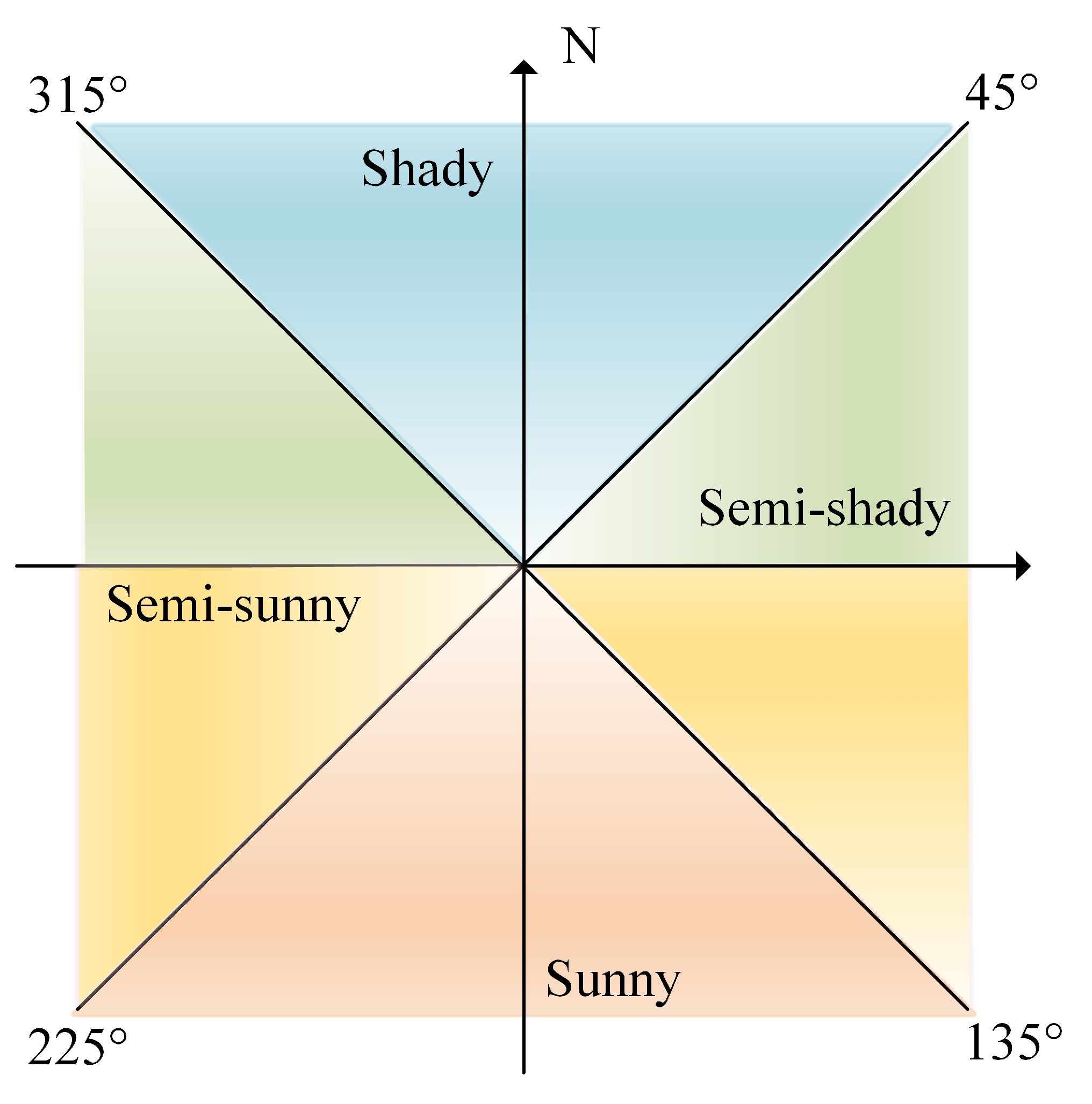
| Class | Range (°) | Directions | Proportion (%) | Variables |
|---|---|---|---|---|
| 1 | 45–90, 270–315 | Semi-shady | 26.180 | SA1 |
| 2 | 90–135, 225–270 | Semi-sunny | 25.109 | SA2 |
| 3 | 0–45, 315–360 | Shady | 24.177 | SA3 |
| 4 | 135–225 | Sunny | 24.534 |
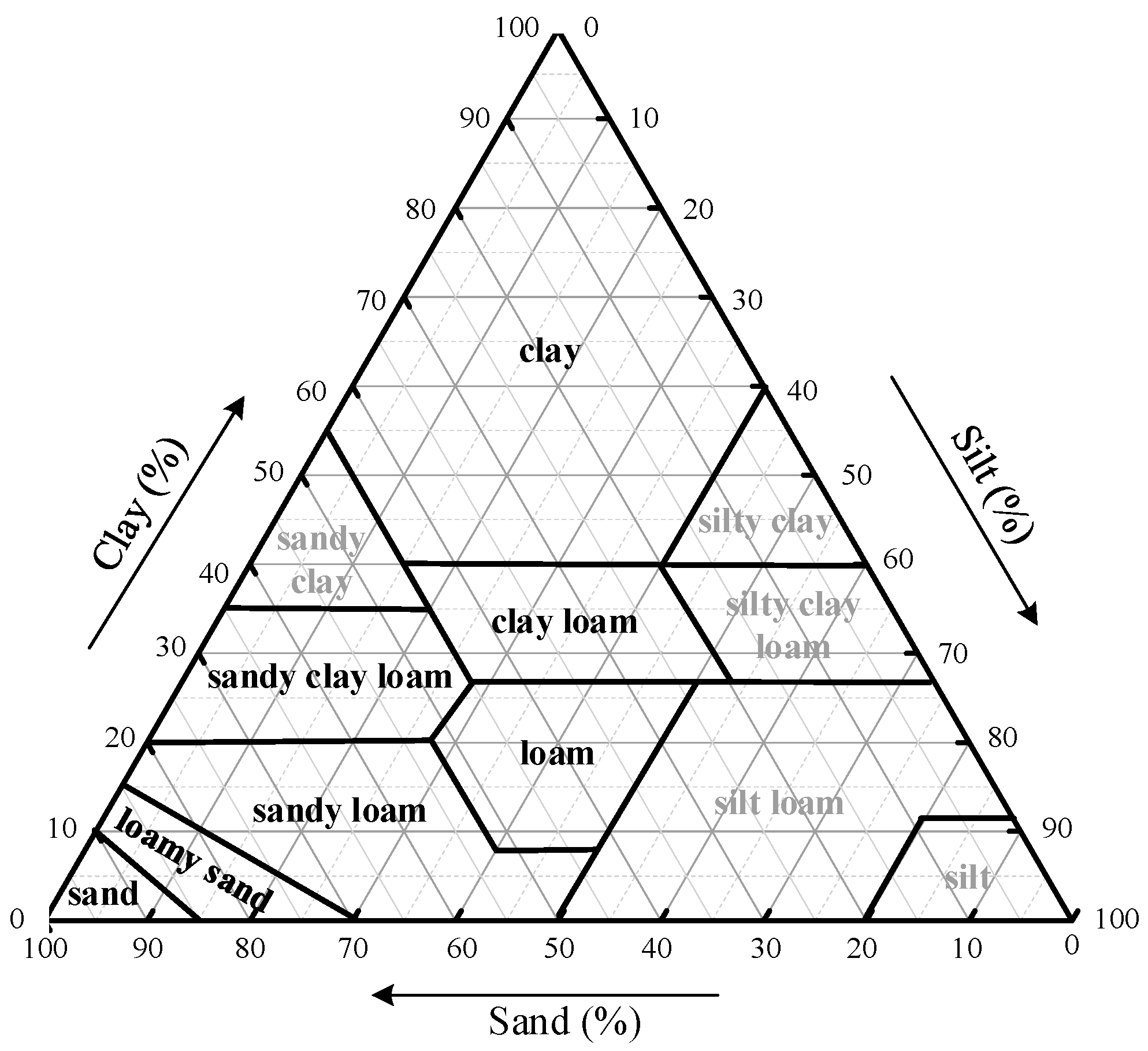
| Class | Soil Texture | Proportion (%) | Variables |
|---|---|---|---|
| 1 | Silt | - | - |
| 2 | Silt loam | - | - |
| 3 | Loam | 34.292 | ST1 |
| 4 | Silty clay loam | - | - |
| 5 | Clay loam | 1.088 | ST2 |
| 6 | Silty clay | - | - |
| 7 | Clay | 0.206 | ST3 |
| 8 | Sandy clay loam | 2.531 | ST4 |
| 9 | Sandy clay | - | - |
| 10 | Loamy sand | 10.017 | ST5 |
| 11 | Sand | 0.373 | ST6 |
| 12 | Sandy loam | 51.493 |
| Period | In Calibration | In Validation | ||
|---|---|---|---|---|
| No. of Samples | Proportion 1 (%) | No. of Samples | Proportion 1 (%) | |
| Annual | 7484 | 0.241 | 7493 | 0.242 |
| Winter | 6771 | 0.255 | 6763 | 0.254 |
| Spring | 6891 | 0.222 | 6879 | 0.222 |
| Summer | 6419 | 0.214 | 6415 | 0.214 |
| Autumn | 7415 | 0.248 | 7418 | 0.248 |
| Period | Regression Model | Adj. R2 | RMSE | Max VIF |
|---|---|---|---|---|
| Annual | RSM = 125.231 − 0.294*DL + 24.804*DVI − 0.114*NL + 0.004*PRE + 2.409*DEM1 + 0.884*DEM2 + 0.277*DEM4 + 0.552*DEM5 + 0.726*DEM6 + 0.632*LC1 + 0.398*LC2 + 0.144*SG3 + 0.163*SG4 + 0.237*ST1 + 1.826*ST3 − 1.607*ST4 − 0.721*ST5 | 0.572 | 1.698 | 2.993 |
| Winter | RSM = −226.027 + 0.806*DL + 20.709*DVI + 0.032*ET + 0.030*NL − 0.014*PRE + 0.052*RH + 0.239*DEM2 − 0.263*DEM4 − 0.155*DEM5 + 0.185*DEM6 + 0.215*LC1 + 0.174*SG2 + 0.297*SG3 + 0.296*SG4 + 0.277*SG5 + 0.086*ST1 + 0.983*ST3 − 0.998*ST6 | 0.912 | 0.798 | 2.195 |
| Spring | RSM = 195.013 − 0.564*DL − 0.059*NL + 0.019*PRE + 3.504*DEM1 + 1.750*DEM2 − 0.590*DEM5 − 0.760*DEM6 + 1.255*LC2 − 0.300*SG3 + 0.201*ST1 − 0.779*ST2 − 1.122*ST4 − 0.710*ST5 | 0.540 | 2.978 | 2.428 |
| Summer | RSM = 193.779 − 6.122*DVI + 0.340*ET − 0.650*NL + 0.012*PRE + 2.152*DEM1 + 0.895*DEM2 − 0.728*DEM5 + 2.484*LC2 + 0.429*SG4 + 0.891*SG5 + 0.518*ST1 + 1.063*ST2 + 2.591*ST3 + 0.676*ST4 − 1.962*ST5 | 0.592 | 3.834 | 2.242 |
| Autumn | RSM = −45.187 + 0.187*DL + 16.927*DVI + 0.285*ET + 0.006*PRE + 1.886*DEM1 + 1.095*DEM2 + 0.151*DEM4 + 0.375*DEM5−1.657*LC2 + 0.457*SG2 + 0.520*SG3 + 0.338*SG4 − 0.828*ST4 − 0.301*ST5 | 0.283 | 2.202 | 2.366 |
| Period | In Calibration 1 | In Validation 1 | ||
|---|---|---|---|---|
| Adj. R2 with Dummy Variables | Adj. R2 without Dummy Variables | Adj. R2 with Dummy Variables | Adj. R2 without Dummy Variables | |
| Annual | 0.572 | 0.505 | 0.565 | 0.497 |
| Winter | 0.912 | 0.908 | 0.912 | 0.908 |
| Spring | 0.540 | 0.515 | 0.531 | 0.501 |
| Summer | 0.592 | 0.647 | 0.566 | 0.625 |
| Autumn | 0.283 | 0.227 | 0.272 | 0.215 |
Publisher’s Note: MDPI stays neutral with regard to jurisdictional claims in published maps and institutional affiliations. |
© 2021 by the authors. Licensee MDPI, Basel, Switzerland. This article is an open access article distributed under the terms and conditions of the Creative Commons Attribution (CC BY) license (https://creativecommons.org/licenses/by/4.0/).
Share and Cite
Yuan, L.; Li, L.; Zhang, T.; Chen, L.; Liu, W.; Hu, S.; Yang, L. Modeling Soil Moisture from Multisource Data by Stepwise Multilinear Regression: An Application to the Chinese Loess Plateau. ISPRS Int. J. Geo-Inf. 2021, 10, 233. https://doi.org/10.3390/ijgi10040233
Yuan L, Li L, Zhang T, Chen L, Liu W, Hu S, Yang L. Modeling Soil Moisture from Multisource Data by Stepwise Multilinear Regression: An Application to the Chinese Loess Plateau. ISPRS International Journal of Geo-Information. 2021; 10(4):233. https://doi.org/10.3390/ijgi10040233
Chicago/Turabian StyleYuan, Lina, Long Li, Ting Zhang, Longqian Chen, Weiqiang Liu, Sai Hu, and Longhua Yang. 2021. "Modeling Soil Moisture from Multisource Data by Stepwise Multilinear Regression: An Application to the Chinese Loess Plateau" ISPRS International Journal of Geo-Information 10, no. 4: 233. https://doi.org/10.3390/ijgi10040233